Identification of shallow cracks in rotating systems by utilizing convolutional neural networks and persistence spectrum under constant speed condition

1. Introduction

During the last century not only has been increased the use of rotating machines noticeably but also faults detection methods in these instruments have been witnessed significant improvements. Since a wide range of rotating systems work in places that are difficult to access such as offshore wind turbines, and many of these systems carry heavy appurtenances such as blades, automated and early fault identification processes play an important role in decreasing cost, time, and human injuries. Although various types of defects can occur in rotor systems such as unbalance, shaft cracks, misalignment, fluid-induced instability, bearing failure, rub/looseness, blade cracks, and shaft bow, some of them such as shaft cracks are more prevalent, also their late detection can bring about catastrophic failures. Since many of these faults in their advanced stages have similar symptoms in the methods that researchers have introduced so far, the priority belongs to the procedures that can detect defects in their very early stages where the negligible abnormality can be seen properly.

In the course of the defect, we are examining in this paper, i.e. cracks in the shaft, frequency domain, and time-frequency transformations such as Fourier transform and wavelet transforms have shown reasonable capability. Since the interpretation of vibration signals and their transformations needs high-level knowledge and experience, introducing self-administered faults identification processes that are useable by medium-level technicians has attracted many researchers' attention during the recent decade. One of these methods is named classification where a pre-trained network can distinguish various defects in different severities automatically. Parallel with remarkable advancements in the graphical units of computers, scientists tend to deal with methods based on graphical data because as will be mentioned later, these types of data can be employed in creating self-acting faults detection procedures more conveniently. One of the sophisticated graphical-based classification methods is convolutional neural networks (CNNs) that are a type of artificial neural network employed in image recognition and image processing.

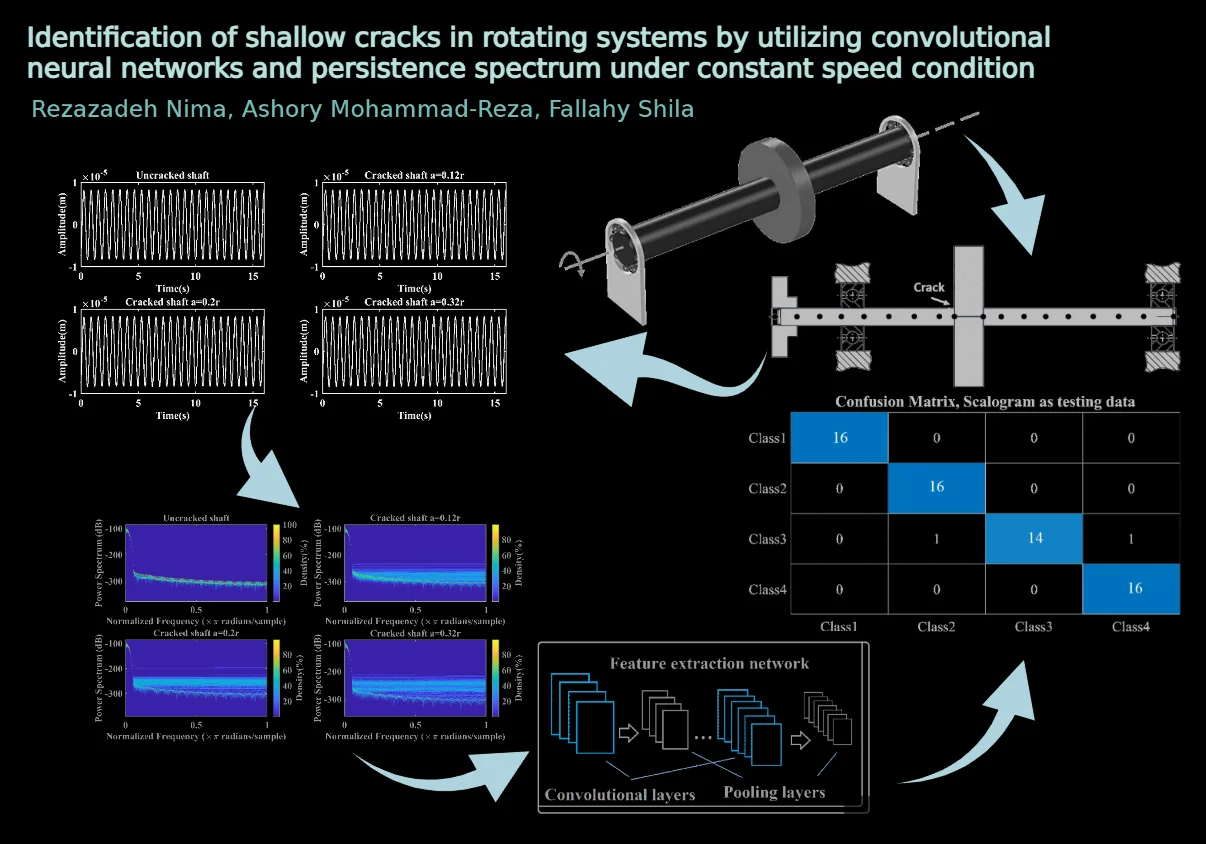
In the present work, a hybrid method is used to classify cracked rotors with shallow depths from healthy ones throughout the steady-state operation. To train a deep network based on CNNs, persistence spectrum images are used as input data. These images are obtained by converting the raw signals of the time domain into the frequency scope. To begin with, the finite element method is used to model healthy and cracked rotor systems. By reading the literature in this field, authors are aware that this combined method, i.e. CNNs and persistence spectrum have not been used by the other scientists in the classification of cracked rotors in steady-state operation; in addition, the obtained accuracy revealed that this method can be considered as a reliable procedure in the identification of cracked rotor systems with various depths.

2. Previous works

Studies on the dynamics of cracked rotor systems have been developed by many scholars since 1986 when Nelson and Nataraj investigated the effect of a transverse crack on the stiffness matrix of a rotating machine [1].

Extensive reviews on the newest crack detection methods in rotating systems can be met in Kumar et al. [2], and Kushwaha et al. [3]. Concerning the detection of cracks in rotors, Saavedra and Cuitino proved that due to the presence of a crack in a shaft, stiffness is reduced and consequently the natural frequencies of the system are diminished [4].

Modeling the breathing behavior of a crack in the rotor system is not a new concept, since according to Papadopoulos and Dimarogonas if a cracked shaft rotates slowly under its weight, the crack opens and closes, that is, it breathes. This behavior was modeled using a truncated cosine function [5]. The effect of this phenomenon is also used by scholars as an indicator of the crack in rotatory machines where Alzarooni et al. showed the appearance of the postresonance backward whirl is a symptom of breathing crack [6].

Signal processing of cracked rotary systems is usually considered in two different operating conditions, namely transient and steady-state. Sekhar and Prabhu worked on the transient signals of a cracked rotor when it was passing through its first critical speed; the crack was assumed to be a transverse type. Continuous wavelet coefficients were used in demonstrating various factors on crack’s condition such as depth, start-up acceleration, and unbalanced eccentricity. In the article, it was assumed that because of a crack some sub-harmonic phenomena appeared before the first critical speed in wavelet coefficients’ plots [7].

Gómez et al. studied cracked rotors characteristics in both theoretical and empirical operation conditions. In the theoretical modeling, it was assumed that the system was a Jeffcott rotor (with a central rotating disk and with inflexible bearings). Noticeable variations in energy levels were observed at first, second, and third harmonics. On the other side, in experimental investigation, nine crack situations were exerted in the rotor. Comparing theoretical and experimental outcomes, it was asserted that merely components could be the evident sign of the crack in analyzing steady-state operation [8].

Rezazadeh studied both of these operational conditions in cracked systems by utilizing Fourier and continuous wavelet transformations. In this article, the capacities of frequency and time-frequency methods in distinguishing cracks are compared with each other. In the case of transient signals, CWT revealed great aptitude while for the steady-state operation Fourier transform showed enough capability in divulging crack symptoms [9].

One of the successful derivatives of artificial intelligence is machine learning; deep learning is a branch of machine learning that its ability in speech recognition [10], image processing [11], and natural language comprehension [12] has proved successful. Briefly, artificial intelligence intends to emulate the human brain’s ability in interpreting data.

Classification of crucial signals such as EEG and ECG has been developed by many scholars during these two last decades. Ling Gue et al. used the concept of relative wavelet energy (RWE) informing the feature vector in the classification of normal and epileptic signals [13]. After that, Kumar et al. employed the RWE and wavelet entropy (WE) in creating the feature vector to classify normal and abnormal EEG signals [14].

Rezazadeh and Fallahy used these two features, i.e. RWE and WE to form the feature vector and then classify cracked rotors from healthy ones. By applying discrete wavelet transformation (DWT), cracked and healthy rotors were decomposed until level 6. Db 32 as the mother wavelet function and a multi-layer Perceptron network were used in the classification method [15].

In recent years, the use of convolutional neural networks in fault diagnosis has increased significantly. In experimental work, Zhao et al. first removed unwanted disturbances from the collected signals using noise removal methods such as variational mode decomposition (VMD) and probabilistic principal component analysis (PPCA), then classified cracked and misaligned rotating systems [16].

In this paper, a CNN is developed in distinguishing shallow cracks in the rotary system during steady-state operation. The proposed procedure in this work consists of the below steps:

1) The healthy and cracked systems with three depths are modeled accurately by utilizing the finite element method (constituting breathing behavior) in MATLAB.

2) Solving the system's equation of motion with various conditions numerically.

3) Calculating the achieved signals' persistence spectrum and save these images.

4) Allocating the main parts of spectrums as the training part and the remaining as the testing section.

5) Training the convolutional neural network with the inputs and testing the efficiency of the trained network.

3. Materials and methods

3.1. Modeling the rotating system

Like all damped vibrating systems, for a de Laval rotor model the equation of motion can be introduced as below:

1

$\left[M\right]\left\{\ddot{U}\right\}-\mathrm{\Omega }\left[C\right]\left\{\dot{U}\right\}+\left[K\right]\left\{U\right\}=\left\{Q\right\},$

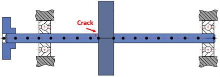
In the above equation, $M$, $C$, $K$, and $Q$ are the system’s mass, damping, stiffness, and force matrices, respectively. Moreover; $U$, $\dot{U}$, and $\ddot{U}$ are the system’s displacement, velocity, and acceleration vectors, ordinary. In Fig. 1 the assumed de Laval rotor and the applied nodes to the Timoshenko beam element, also the crack location is represented.

Fig. 1De Laval rotor system’s schematic

In [9], the system’s characteristic matrices for healthy and cracked systems were introduced and in current work those results are employed. If the flexibility matrix of a healthy element is $\left[C_{uc}\right]$, then the total flexibility matrix of the element that is suffering a crack $\left[C_o\right]$ can be introduced as the sum of the healthy element’s flexibility matrix and additional flexibility that is resulted from the crack, in the form of:

2

$\left[C_o\right]=\left[C_{uc}\right]+\left[C_c\right].$

Here $\left[C_c\right]$ contains the additional flexibility that is caused due to crack in an element and can be introduced as:

3

$C_c=\frac{1}{F_0}\left[\begin{array}{cccc}{\stackrel{-}{c}}_{22}r& 0& 0& 0\\ 0& {\stackrel{-}{c}}_{33}r& 0& 0\\ 0& 0& {\stackrel{-}{c}}_{44}/r& {\stackrel{-}{c}}_{45}/r\\ 0& 0& {\stackrel{-}{c}}_{54}/r& {\stackrel{-}{c}}_{55}/r\end{array}\right].$

In the above equation, ${\stackrel{-}{c}}_{45}={\stackrel{-}{c}}_{54}$; the amount of $F_0$ is stated in [17]. The elements of $\left[C_c\right]$ are calculated from the relations that are introduced in [18], and also the obvious remarks that are stated in [19] and in the Wolfram Mathematica. It should be noted that these are non-dimensional and only are related to the crack’s depth and can be used for all cracked-rotor systems with different mechanical and electrical properties. After calculating the flexibility matrix for a cracked element by multiplying the total flexibility matrix of the cracked element, i.e. $\left[C_o\right]$, in a transformation matrix, $\left[T\right]$, stiffness matrix for a cracked element can be obtained. Similarly, for a healthy element by multiplying the transformation matrix in $\left[C_{uc}\right]$ the related stiffness matrix can be achieved [18].

To model the breathing behavior of a crack in the rotary system, the results from [5] is applied, so the stiffness matrix of a cracked element with regarding its breathing behavior can be introduced as:

4

$\left[K\right]=\sum _{j=0}^n\left[K_j\right]\cos j\omega t.$

In Eq. (4), by selecting a higher number of sentences, i.e. “$j$”, the accuracy can be increased, but by choosing the higher number of sentences the higher boundary conditions (B.C.) are needed. In this work, four sentences are selected; B.C. is introduced as following where $\mathrm{\varnothing }=\omega t$, $\omega$ is the shaft angular velocity, ${\left[K\right]}_{OP}$ and ${\left[K\right]}_{UN}$ are the open crack and healthy shaft stiffness matrices respectively:

5

$B.C.\to \left\{\begin{array}{c}at\varnothing =0\to \left[K\right]={\left[K\right]}_{UC},\\ at\varnothing =0\to \frac{{\partial }^2}{\partial {\varnothing }^2}\left[K\right]=0,\\ at\varnothing =\pi \to \left[K\right]={\left[K\right]}_{OP},\\ at\varnothing =\pi \to \frac{{\partial }^2}{\partial {\varnothing }^2}\left[K\right]=0.\end{array}\right.$

3.3. Signal processing

This step plays a crucial role in the quality of almost all classification procedures. In many cases, the vibration signals of faulted and healthy systems seem to be very close to each other, so the raw signal should be processed before the appropriate features will be extracted from it. Also in experimental works, this stage constituting noise cancellation proceedings. Concerning the intrinsic nature of the signal, various methods can be employed in this step from simple noise-cancellation to sophisticated multi-steps time-frequency transformations. Time-frequency processes can be account as very capable methods in distinguishing hidden changes in the transient vibration signals especially when there is a nonlinear disturbance such as breathing crack. On the other hand, in a vast variety of prior investigations it is proved that in the steady-state operation Fourier transform can be considered as a reliable method in identifying cracks in shaft [3].

In this work, the persistence spectrum that is a time-frequency presentation of the Fourier transform is applied in the signal processing step. The persistence spectrum of a signal is a frequency display that represents the portion of time that a certain frequency exists in a signal in percent. This method can reveal latent frequency characteristics in a signal by coloration, hotter coloration more frequency severity. This is a histogram in power-frequency space. To draw the persistence spectrum of a signal such as “Y” in MATLAB, it is enough following code will be performed:

%pspectrum (Y, ...

%'persistence', ...

%'FrequencyLimits',frequencyLimits, ...

%'TimeResolution',timeResolution, ...

%'OverlapPercent',overlapPercent);

Fig. 3 represents the capability of the persistence spectrum in revealing symptoms that are latent in the time-domain graphs, i.e. Fig. 2; in addition, to have a comparison between other time-frequency domain transformations, continuous wavelet transformation (using FFT), and the detail coefficients of discrete wavelet transformation in Fig. 4, Fig. 5, Fig. 6, and Fig. 7. All of these diagrams are plotted for systems similar to the parameters shown in Table 1. In addition, the diagrams have belonged to three systems suffering cracks with relative depths equal to $a=0.12r$, $a=0.2r$, and $a=0.32r$ and one healthy during the steady-state operation.

Fig. 2Time-domain signals for the healthy and cracked shafts

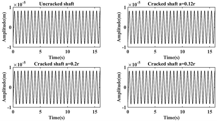
From Fig. 2 can be understood that the graphs of time-domain signals are not able to represent any useful information because in the above figure any sudden change or discrepancy in the amplitude cannot be observed. This is caused by the fact that the cracks’ depths are shallow, also system works after its first critical speed and relatively stable condition. In the following, and Fig. 3 persistence spectrum graphs are drawn for the same signals.

Table 1Mechanical properties of the rotor system

Property	Amount	Property	Amount	Property	Amount
Disc’s mass	4 kg	Shaft’s modulus of elasticity	2.08 e11 Pa	Shaft’s angular velocity	10 rad/s
Disc’s eccentricity	3e-3	Shaft’s length	1 m	Bearing’s damping	100 N/m
Shaft’s density	7780 kg/m3	Shaft’s diameter	3 e-1 m	Bearing’s stiffness	1e5 N/m

Fig. 3Persistence spectrums for the healthy and cracked shafts

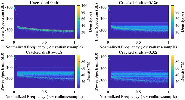
Fig. 3 shows many visible differences for these systems, by increasing the crack’s depth, the number of lines in the higher frequencies experienced a significant rise even for the cracked shaft with relative depth $a=0.12r$ these changes can be seen obviously.

In Fig. 4 and Fig. 5, the graphs for continuous wavelet transformation (CWT) are displayed. It should be noted that the non-analytic Morlet wavelet (morlex) is used as the wavelet mother function, this function is applied because it has revealed the best resolution beyond all the tried functions. In the first step, the sampling period is selected as 0.5 because by choosing a greater sampling period the Modulus, Real part, and Imaginary part could not be represented properly. Moreover, because in this method the changes in the graphs were not very visible, only for the healthy and the shaft with the highest crack depth, i.e. $a=0.32r$, CWT coefficient are plotted. In Fig. 4(b), the sampling period is increased from 0.5 to 2, and the number of parameters was kept constant, i.e. 6, then the plots related to the angles of CWT coefficients are plotted again.

Fig. 4CWT coefficients (sampling period = 0.5) for healthy and the cracked shaft with a=0.32r

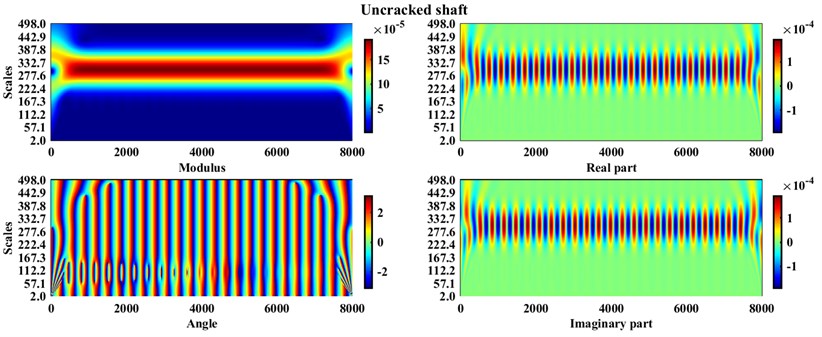
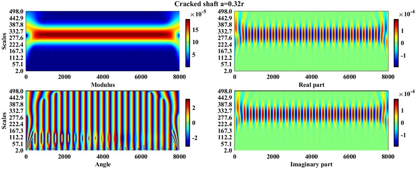
Fig. 5Angles of CWT coefficients (sampling period = 2) for the healthy and cracked shaft with a=0.32r

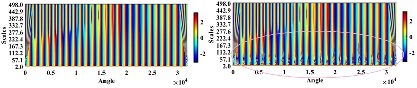
From Fig. 4 and Fig. 5 it can be concluded that except for the angles of the CWT coefficients at the higher sampling frequency, i.e. 2, which at the lower scales (marked with a colored circle in Fig. 5) show some changes for healthy and cracked shafts, the diagrams of other parts of the wavelet coefficients cannot show a noticeable difference.

Now, for the last part of the comparison, details of discrete wavelet transformation (DWT) are presented in Fig. 6 where the signals in Fig. 2 are decomposed until level 3, and by using Symlet-4 as the mother wavelet function.

Since at the beginning and end of the above plots there is a relatively great amplitude in the amounts of details, the changes in the other parts of the diagrams cannot be seen appropriately. By limiting the horizontal axis between 0.245 and 15, the changes can be observed more properly, so in Fig. 7 the zoomed graphs are plotted for detail level1 (Detail 1).

Fig. 6Details of DWT in the three levels for the healthy and cracked shafts

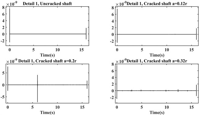
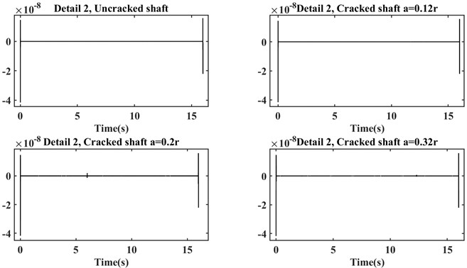
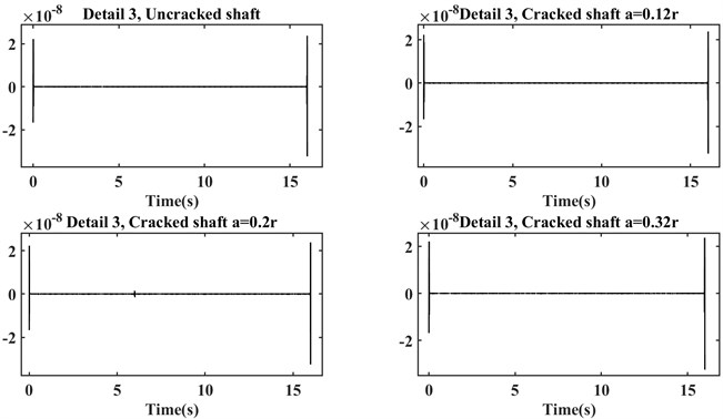
Fig. 7Detail 1 of DWT with the limited horizontal axis

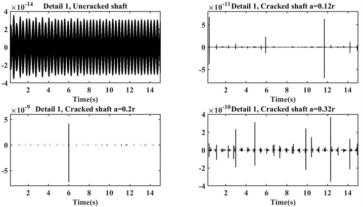
As it is mentioned before, by limiting the horizontal axis, changes in the detail plots of the four shafts can be seen properly. Although the changes in the detailed plot of the healthy shaft are more visible, its amplitude is very lower than the cracked shafts.

3.4. Convolutional neural networks (CNNs, ConvNet)

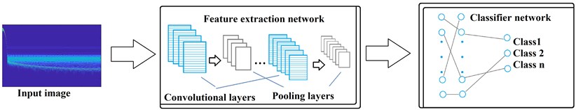
Briefly, image recognition can be introduced as classification. For image recognition that revived since 2012 [21], CNN is a deep neural network that can be considered as an especial tool. Fig. 8 shows the operation process of the ConvNet. In the first stage, the input images arrive at the feature extraction network, which in itself consists of two series of different layers, namely the Convolutional layer and the Pooling layer. The extracted features are then entered into a classification neural network. In the last step, the classifier network classifies input images according to the extracted features from them.

The main benefit of ConvNet in comparison to the other machine learning methods is that this procedure can automatically detect the significant features of various images while in the other processes firstly a feature vector should be introduced where can be a difficult task in many cases. In industrial cases, only the proper graph that can be achieved of time, frequency, or time-frequency transformations can be used as the input data to the CNN.

Fig. 8Common structure of a ConvNet

It should be noted that between the convolutional layer and pooling layer a transfer (activation) function is needed to translate the input signals to output signals. Various types of activation functions have been introduced by scholars, but some kinds of them are more prevalent than the other, i.e. sigmoid, Gaussian, Rectified Linear Unit (ReLU), and piecewise linear.

As a result of the benefits that have been stated for ConvNet, the use of this sophisticated method has increased dramatically in recent years in all fields from medicine to industry. As an illustration of that, in Table 2, three recent works that applied the CNN in fault diagnosing in rotating systems are represented.

Table 2Recent articles that have applied CNN in fault diagnosis in rotor systems

Author(s)	Type(s) of images	Type(s) of fault	Year
Myungyon Kim et al. [22]	Vibration images	Rubbing, misalignment, and oil-whirl	2020
Jiangquan Zhang et al. [23]	Time-domain signals	Bearing fault	2020
Clayton Rodrigues et al. [24]	Spectral image of Vibration Orbits	Unbalance, misalignment, shaft crack, rotor-stator rub, and hydrodynamic instability	2021

From Table 2 it can be concluded that CNN is a successful method of troubleshooting in rotating systems. The innate nature of the crack, i.e. short-term propagation, has encouraged the authors of this paper to use CNN to identify shallow cracks in the rotating system.

In this work, ReLU is employed because this function can increase the speed of convergence, decrease the issue of the low-speed of parameters updating and the vanishing gradient [25]. An AlexNet that is a ConvNet consisting of 25 layers is applied as the convolutional neural network. Table 3 represents the architecture of AlexNet.

Table 3The architecture of used AlexNet

No. of layer(s)	Name of layer	No. of layer(s)	Name of layer	No. of layer(s)	Name of layer
1	Image Input	4, 8	Cross-Channel Normalization	19, 22	Dropout
2, 6, 10, 12, 14	Convolution2D	5, 9, 16	Max Pooling2D	24	Softmax
3, 7, 11, 13, 15, 18, 21	ReLU	17, 20, 23	Fully Connected	25	Classification output

4. Results

For three cracks’ depths equal to $a=0.12r$, $a=0.2r$, and $a=0.32r$ and without crack, operational conditions, i.e. angular velocity, and the innate parameters, i.e. disc’s mass, eccentricity, bearings’ stiffness, damping ratio, shaft’s density, length, diameter, and elasticity modulus have changed randomly, then vibration signals are captured during 16 seconds of the steady-state operation. These changes caused we could have 440 systems, on the whole, i.e. 110 for each health condition. Class 1, Class2, Class 3, and Class 4 are indicators of healthy, cracked $a=0.12r$, cracked $a=0.2r$, and cracked $a=0.32r$ shafts respectively.

The persistence spectrum of these signals is stored. 85 % of the data (images) were randomly selected for the training phase, and the rest of the images were allocated for the testing step.

In the network, the image sizes are equal to 227×227; for better results, the title of the graphs, and the number details related to the axes have been removed automatically. The number of the maximum epoch is selected equal to 15, the mini-batch size tantamount as 12, and the initial learning rate equals 1e-4.

After training and testing stages, the below confusion matrix shows the accuracy of our supervised convolutional neural network.

Fig. 9Confusion matrix, scalogram as testing images

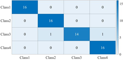
From Fig. 9 it can be seen that the trained convolutional neural network represented a reasonable accuracy in identifying the 4 classes, i.e. with accuracy equal to 97 %. This network only has confused in separating 2 samples that belonged to Class 3, one of them has distinguished to be in Class 2, and the other mistakenly identified to be in Class 4. This is because all of the cracked shafts suffering relatively shallow depths and their persistence spectrums were very similar to each other in some operational and physical conditions; on the other hand, the noticeable positive point about the network is that it can distinguish the shallowest crack depth, $a=0.12r$ from the other classes correctly. While this method can be somehow time-consuming in the case of a single CPU, this issue has been resolved properly by employing a Graphic processing unit (GPU). It should be mentioned that although in some previous works that have been classified cracked shafts from healthy ones the achieved accuracy was higher than the accuracy in this work, firstly this paper has worked on the shallow cracks identifying and this can result in similar behavior in some cases, secondly, in this method, we do not require to introduce and form a proper feature vector (in some cases this task can be a very hard task) and the network automatically can extract the features from images.

To have a comparison between the operation of various transfer functions, the network has trained and tested with different functions by replacing in the layers 3, 7, 11, 13, 15, 18, and 21. Table 3 presents the accuracies that have been achieved by employing Hyperbolic tangent (tanh), Leaky Rectified Linear Unit (Leaky ReLU), and Exponential linear unit (ELU).

From Table 4 it can be understood that in our ConvNet, ReLU showed higher accuracy than the other activation functions; in addition, the required time to convergence was fewer than the other functions.

5. Conclusions

To begin with, the characteristic matrices and the local flexibility resulted from cracks of a rotor system are modeled by using results from [9,18]. In the next step, the breathing behavior of the crack is modeled by applying a truncated cosine function and is replaced in each moment of rotation in the global stiffness matrix. The system’s equation of motion is solved by employing Houbolt time marching that is a numerical procedure, and the systems' steady-state responses are calculated during 16 seconds of their operations. In the signal processing stage, some methods are compared with each other in revealing hidden frequency parameters in the raw signal and finally, the persistence spectrum is selected as the appropriate transformation. The modeled systems are run for various physical and operational circumstances and each class, i.e. Class 1, Class 2, Class 3, and Class 4 exactly 110 sample signals and persistence spectrums are calculated and the persistence spectrums are saved as the data. In the final step, an AlexNet that is a convolutional neural network with 25 layers is chosen as the network. 85 percent of data, i.e. images are allocated to the training step, and the other 15 percent of them are introduced as the data for the testing process. The acquired accuracy, 97 %, offers the supervised ConvNet as a proper method in the classification of cracked rotors with various depths from the healthy one.

Despite crucial signals where different real-time normal and abnormal data exist and scientists can examine the trained deep neural networks with them, engineering fields suffer this leakage. As a result, for future works, a test rig can be designed and the trained network in this method can be examined with real-time data.