Abstract
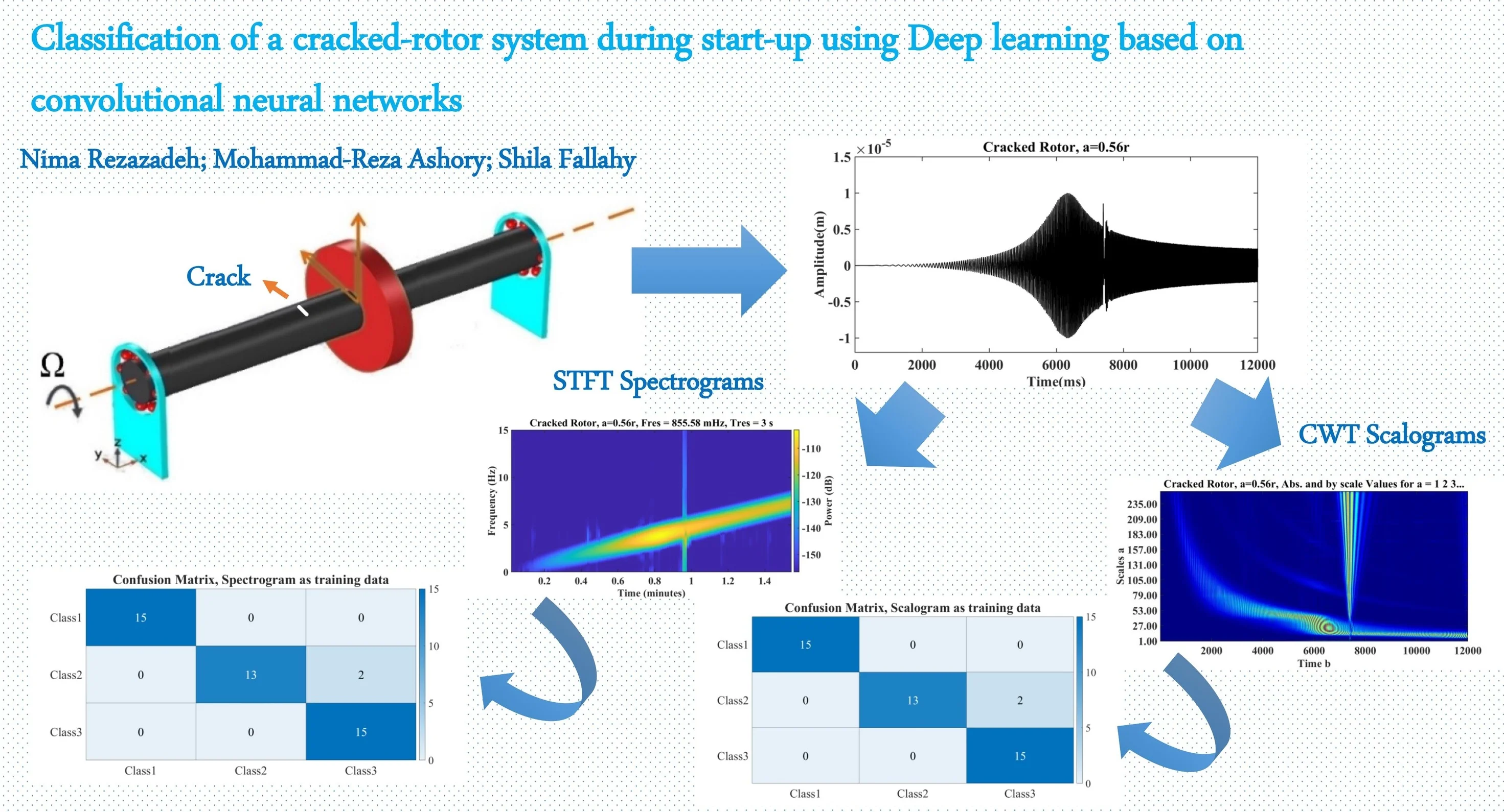
This article addresses an improvement of a classification procedure on cracked rotors through Deep learning based on convolutional neural networks (CNNs). At first, a cracked rotor-bearing system is modeled by the finite element method (FEM), then throughout its start-up, the related time-domain responses are calculated numerically. In the following, as a pre-processing stage, continuous wavelet transform (CWT) and Short-time Fourier transform (STFT) are applied on the three various health conditions, i.e. without crack, shallow-cracked, and relatively deep-cracked shafts. The plots of CWT’s coefficients and STFT’s in these various classes are used as the input dataset in Deep learning based on CNNs and the three classes are introduced as the output. AlexNet with 25 layers is employed as the network. The results of the testing phase demonstrated that not only this expanded method has a reasonable capacity in the classification of cracked and healthy rotors, but it also can classify cracked rotors with different crack depths with a negligible error.
Highlights
- Early fault classification can result in more precise and cost-effective maintenance.
- Transient signals are carrying beneficial information in regard to the health situation of rotating systems.
- Having knowledge concerning how much a fault can be dangerous can give the ability to the condition monitoring personnel to stop devices at the appropriate time.
- The graphs of time-frequency transformations can reveal hidden signatures of various failures.
- Convolutional neural networks can extract features from time-frequency graphs and use these features for the training and testing steps.
- The trained network can be saved and utilized for other similar purposes.
1. Introduction
In the course of a noticeable increase in energy consumption that is an ineluctable conclusion of the industrial revolution, effective maintenance of energy conversion appliances has become a favorite field in scientific investigations. To mention the importance of rudimentary faults identification in energy transformer instruments it is enough to say that delayed recognition of deficiencies can bring about catastrophic repercussions both in the labor force and cost. One of the most common machines in the energy field is the rotor system that normally operates at a high pace, and a large amount of high-price appurtenances are attached to it. A usual rotor system consists of a central rotating shaft, blade (turbine blade), engine motor, and supporters such as bearings. Rotating systems are suffering from a wide range of mechanical and electrical faults such as unbalance, crack, rotor to stator rub, misalignment, and things like these areas. Besides unbalancing and misalignment, crack accounts as a prevalent deficiency in the rotor system. Because of the nature of this defect, i.e. can result in breaking down and serious damages to other rotating parts such as blades, this mysterious imperfection should be realized in its early stages. Many factors can involve in creating a crack and this fault can be categorized with consideration of its angle with the shaft’s central axis, or its depth.
In the present research, a Deep learning procedure based on CNNs is used in the classification of healthy and cracked rotor systems with disparate crack depths. As the pre-process step, continuous wavelet transform and Short-time Fourier transform are exerted and the saved scalograms and spectrograms are introduced as input to the training process, and finally, the supervised network classifies the plots according to the rotor’s health conditions in three categories. As the authors of this paper know any other researcher has not been using CNNs with time-frequency plots as the training dataset in the classification of cracked rotor systems.
2. Previous works
During recent years many researchers have worked on the various crack identification processes from analyzing time-domain responses to more sophisticated methods such as time-frequency procedures. Crack identification methods can be divided into various scopes, but two comprehensive classes are local and global procedures. Although some local procedures such as NDT can distinguish cracks in static mode, their disabilities in online crack identification propel scientists in developing and applying global procedures such as signal processing [1].
Sekhar and Prabhu investigated the transient responses of a cracked rotor when it was crossing through the first critical speed; the crack was assumed to be a transverse type. To model the breathing behavior of the crack, a simple hinge model was considered. Continuous wavelet coefficients were used in demonstrating various factors on crack’s condition such as depth, start-up acceleration, and unbalanced eccentricity. In the paper, it was claimed that due to the presence of a crack some sub-harmonic phenomena appeared before the first critical speed in wavelet coefficients’ plots [2].
In 2016, Sekhar et al. compared different time-frequency methods in distinguishing three various defects, i.e. crack, misalignment, and rotor to stator rub in the rotating system. To do this, Sekhar calculated time-domain responses of the modeled systems that were suffering the three faults, then processed the vibration signals when the systems were crossing across their first critical speeds utilizing Hilbert-Huang transformation (HHT), STFT, and CWT. Sekhar asserted that CWT is a reliable tool in analyzing noisy signals while HHT is a more rapid transformation in online monitoring [3].
In 2016, Söffker et al. compared an older procedure, model-based, and a newer one, signal processing based on crack detection in a rotating system. For the former one, the PI-observer-based model was applied; on the other hand, for the latter one, a procedure was exerted based on support vector machine (SVM) and wavelet transform. In the end, the results of the two methods were compared [4].
Gómez et al. studied cracked rotors characteristics in both theoretical and empirical operation conditions. In the theoretical modeling, it was assumed that the system was a Jeffcott rotor (with a central rotating disk and with inflexible bearings). Noticeable variations in energy levels were observed at first, second, and third harmonics. On the other side, in experimental investigation, nine crack situations were exerted in the rotor. Comparing theoretical and experimental outcomes, it was asserted that merely components could be the evident sign of the crack in analyzing steady-state operation [5].
In experimental work, in 2019, Zhao et al. firstly used probabilistic principal component (PPCA) and variational mode decomposition (VMD) to reduce noise from the accumulated signals. In the next stage, feature vectors are extracted for two different systems, a cracked rotor system, and a rotating shaft with misalignment. At the final step, an optimized CNN was applied in classifying the systems [6].
Shah et al. experimented influences of a crack in two circumstances. Firstly, a cracked-rotor system was investigated when the system was suffering unbalancing too. Secondly, the same cracked system was balanced properly and its vibration signals were captured. These two conditions were applied to variation in vibration pattern, and the angle of phase and its value would be observed. The variations in vibration signals are caused by the identification of crack’s properties (i.e. its depth and its place). To have a more obvious vision, a wavelet energy package (WEP) was applied in the introduction of the crack’s location; in the steady-state operation, and was recommended as key factors in crack detection [7].
Rezazadeh and Fallahy applied a hybrid method in the classification of a transversal cracked-rotor system with various crack depths. In this article, the collected vibration signals were de-noised by employing discrete wavelet transform (DWT), then feature vectors were made employing Relative Wavelet Energy (RWE) and Wavelet entropy (WE) concepts. These feature vectors were introduced as the input for a multi-layer Perceptron network. The testing results showed the trained supervised learning classifier had reasonable capacity in classifying various cracked shafts [8].
In 2020, Prabhakar worked on the transient response (during its shut-down) of a slant-cracked rotor system. The vibration signals were collected when the system was passing its first critical speed, and to simulate vibration responses, a finite element method (FEM) for flexural vibrations was applied. To this purpose, a harmonically varying exciting torque plus an arbitrary unbalance force were employed on the modeled rotating system. In this work, Sub-harmonic frequency components with the same properties were revealed in the frequency spectra (FFT graph); in addition, in the case of slant crack, these peaks were located at the critical speed of the rotor-bearing system. To find the crack’s location, the fundamental mode shapes of the rotor systems were processed through wavelet transform. Clearly, at the location of the crack, a peak was perceived in the spatial variation of the wavelet transform’s outcomes [9].
In [10] Kushwaha and Patel prepared a comprehensive review on the crack detection procedures in the rotor system. In this work, all methods that have been used were categorized.
Briefly, in condition monitoring of cracked systems time-frequency procedures revealed higher accuracy and also capacity, because in presence of a crack in a rotating system the creation of some nonlinear components is unavoidable. Time-domain processes are not able to reveal these phenomena especially in transient operations such as start-up or shut-down.
3. Materials and methods
3.1. Rotor-bearing system’s equation of motion
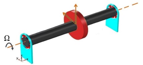
In theoretical analysis, a common rotor system consists of a shaft, disk, and flexible bearings and is shown in Fig. 1. For the assumed system, the equation of motion can be introduced as:
where in the above equation matrices , , are mass, damping, and stiffness matrices respectively; is the force vector and , , and are the displacement, velocity, and acceleration vectors ordinary. To obtain these vectors and matrices, the results of [1, 11] are used; in these sources, the finite element method was employed in calculating mass, damping, and stiffness matrix for a Timoshenko beam element.
Fig. 1Schematic of the assumed rotor-bearing system
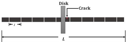
After obtaining the matrices, a transverse crack should be modeled on the shaft. The schematic location of crack is shown in Fig. 2. Existing a crack on the rotor-baring system changes the flexibility of the element containing the crack, so by employing the Strain energy method, the flexibility matrix of a cracked element can be achieved [12, 13]. In this study, a rotor system with 4 degrees of freedom in directions and is assumed.
Fig. 2FEM model of the rotor and crack’s location
If the flexibility matrix of a healthy element is , then the total flexibility matrix of the element that is suffering crack can be introduced as the sum of the healthy element’s flexibility matrix and additional flexibility that is resulted from crack, in the form of:
Here contains the additional flexibility that is caused due to crack in an element and can be introduced as:
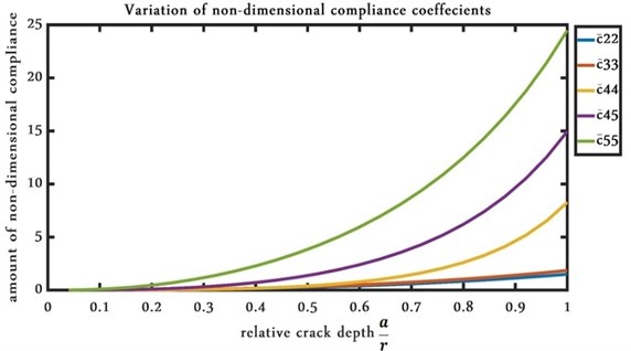
In the above equation, ; the amount of is stated in [14]. The elements of are calculated from the relations that are introduced in [12], and also the obvious remarks that are stated in [15] and in the Wolfram Mathematica. Fig. 3 represents the variations of the elements of the matrix in various crack depths. From Fig. 3 it can be seen that parallel with an increasing in the crack depth, the amount of compliance matrix’s element experienced a rise, too. It should be mentioned that these elements are non-dimensional and only are related to the crack’s depth and can be used for all cracked-rotor systems with different mechanical and electrical properties. After calculating the flexibility matrix for a cracked element by multiplying the total flexibility matrix of the cracked element, i.e. , in a transformation matrix, , stiffness matrix for a cracked element can be obtained. Similarly, for a healthy element by multiplying the transformation matrix in the related stiffness matrix can be achieved [12].
Fig. 3Variation of non-dimensional compliance coefficients by increasing crack’s depth
3.2. Crack breathing behavior
One of the main aspects of a crack in a rotating shaft that separates it from the other common faults is the crack’s breathing behavior. A crack can breathe during its rotation due to its narrow edge and shaft’s heavyweight, so a crack produces nonlinear phenomenon in the vibration responses where its analyzing can be somewhat difficult. During recent years, many investigators have been studying this component. In an early work that until now is authenticated, Papadopoulos assumed that crack’s breathing behavior can be explained by a truncated cosine series [16]. Since that, Darpe [17] modeled breathing behavior utilizing a concept entitled” crack closure line (CCL)”, or in a more sophisticated work, Helen Wu et al. investigated the breathing behavior of a cracked-rotor in consideration to crack’s location. Numerical analysis in Abaqus software was applied to the finite element method’s models. Wu stated that by replacing crack location its breathing mechanism can be changed noticeably [18]. In this work, the proposed method by Papadopoulos [16] is exerted in simulating the breathing behavior.
3.3. Calculation vibration signals
After computing the cracked element’s stiffness matrix and assembling it with the other elements’ stiffness matrices using the finite element method, the rotor system’s total stiffness matrix is obtained. To obtain the system’s responses during its start-up, also forming a dataset as the input of the supervised network, the system’s mechanical and operational conditions have been changed. For instance, the mass of disk is varying between 4 kg to 5 kg, or the initial acceleration in changing from 15 to 115 rad/s2. Other variables are shown in Table 1. It should be noted that because we intend to consider the system when passing its first critical speed, and before the second one, the parameters are selected so that the system does not reach its second critical speed. In addition, system responses are calculated up to 12 seconds from its initial start-up because for the lightest mode, i.e. a 4 kg-disk and the greatest angular acceleration, i.e. 115 rad/s2, this is the maximum time before the system reaches its second critical speed.
Table 1Mechanical properties of the rotor-bearing-disc system
Property | Amount | Property | Amount |
Shaft’s Young’s modulus | 2.08e11 and 2.08e10 Pa | Disc’s mass | 4 to 5 kg |
Shaft’s density | 7780 to 7200 kg/m3 | Disc’s diametral moment of inertia | 0.01546 |
Shaft’s diameter | 3.5 to 2 cm | Disc’s eccentricity | 1e-5 to 3e-4 |
Shaft’s length | 0.5 to 1 m | Bearing’s damping | 85 to 100 N/m2 |
Initial acceleration | 15 to 115 rad/s2 | Bearing’s stiffness | 1e5 and 1.2e5 N/m |
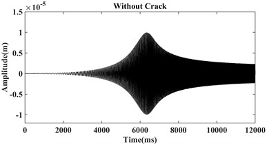
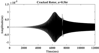
The system equation of motion (Eq. (1)) is solved by numerical Houbolt time-marching procedure with interval 0.001 in MATLAB during the system start-up with the mentioned parameters in the above table, and three different crack’s conditions, i.e. without crack, crack with relative depths 0.32, and 0.56 where is the shaft radius. As an illustration, the vibration signals for the initial acceleration equal to 15 rad/s2, the disc’s eccentricity 0.1e-5 m, disc’s mass 4.4 kg, shaft’s density 7780 kg/m3, damping ratio 100 N/m2 , bearing stiffness 1e5 N/m, shaft diameter 2 cm, Young’s modulus 2.08e11 Pa, and shaft length 0.5 m are plotted in Fig. 4 for the three shafts.
From Fig. 4 it can be seen that by increasing crack depth some sub-harmonic components appeared before and after the first critical speed. Also, for the relatively shallow crack depth (0.32) these changes are not very clear in the time-domain figure and cannot be introduced as a reliable tool in distinguishing crack in rotor system. To cover this deficiency, many researchers have been introducing various methods such as Fourier transform, Short-time Fourier transformation, Hilbert-Huang transformation, and Wavelet transformation that have the efficient capacity in the detection of shallow cracks [10]; in current work, two of these procedures are applied.
Fig. 4Vibration signals of a) healthy, b) cracked with depth a = 0.32r, c) cracked with depth a = 0.56r
a)

b)
c)
3.4. Deep learning
A Machine learning procedure that applies the deep neural network is called Deep Learning. While by adding more layers to the old-fashioned single-layer neural network scientists were expected to witness great improvement in the neural networks’ performance, in the empirical application the accuracy of the neural network decreased comparatively. Deep learning overcame the deep neural network’s three major issues, i.e. vanishing gradient, overfitting, and computational load by exerting suitable learning rules. These three factors were considered as impenetrable barriers to the proper training of deep neural networks [19].
The hidden layers in Deep structured learning can be changed with consideration of the input data and the desired output. One of the well-known Deep Learning architectures is convolutional neural networks (CNNs) that have been exerted to computer vision, machine vision, signal processing, and areas like these. CNNs are considered as powerful and effective tools in classifying visual imagery [20].
Fig. 5Schematic of deep learning and its relationship to deep neural network and machine learning

3.5. Pre-processing of vibration signals
To have a more reliable classification procedure, raw vibration signals should be processed before these signals are located as input in a well-trained multi-layer CNNs. Considering the special nature of the signals in current work where nonlinear components have a great influence on the signals, time-frequency transformations account as powerful tools in the pre-processing stage. One of the efficient time-frequency methods in processing transient signals is continuous wavelet transform (CWT). The CWT of a signal, , is the integral of the signal multiplied by scaled and shifted versions of a wavelet mother function and can be defined by [21]:
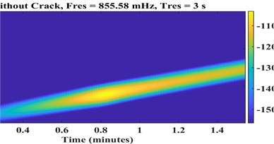
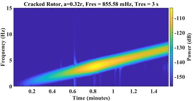
In the above relation and are the shifting and scaling parameters, ordinary; is the time in second. On the other hand, to have a comparison between other time-frequency transformations, the STFT is applied to the signals represented in Fig. 4, too. Short-time Fourier transform is based on the Fourier transform; this procedure divides a high-length signal into short-length sectors with tantamount length and after that calculates Fourier transform on each segment [22]. The STFT of a signal can be described as:
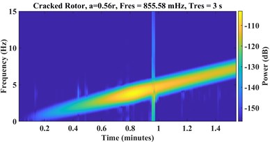
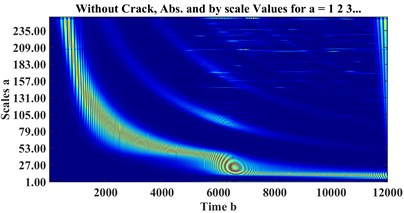
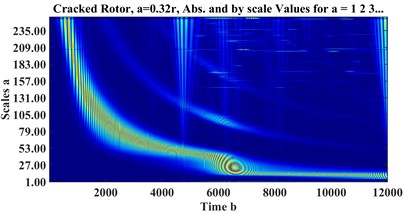
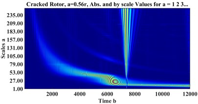
where is the window function, and is the sampling frequency. Fig. 6 and Fig. 7 represent STFT spectrograms and wavelet scalograms, respectively for the signals of Fig. 4. Daubechies 10 wavelet (db10) is selected as the Wavelet Mother function, also scales are limited from 1:256. For STFT, the frequency threshold is selected between 0 to 128 Hz.
Fig. 6STFT spectrograms of a) healthy, cracked with depths b) a = 0.32r, c) a = 0.56r
a)
b)
c)
Since the CNNs method is based on the features extraction from pictorial objects such as images, to have a successful classification procedure, firstly a high-sample database is required. Secondly, the high-resolution images should be introduced as the input for the training step. For these reasons, plots that have been drawn by employing the time-frequency domain transformations can be accounted as trustworthy inputs into CNNs. To do this, two separate CNNs are trained suitably with two different datasets, i.e. CWT scalograms and STFT spectrograms. Three classes, i.e. without crack- Class1, cracked system with relative crack depth 0.32 – Class2, and cracked system with relative crack depth 0.56 – Class3 are considered. For each class 100 samples are obtained from various rotor-bearing-disc systems by the parameters have been mentioned in Table 1. Finally, these two 300-figure sets (300 samples for scalogram and 300 samples for spectrogram) are considered as the dataset.
Fig. 7CWT scalograms of a) healthy, cracked with depths b) a = 0.32r, c) a = 0.56r
a)
b)
c)
4. Results
In current study, a 25-layer AlexNet network is employed as the network. The first layer is Image Input with a dimension 227×227×3, the 23th is Fully connected layer, and the last one is the Classification layer. In addition, Softmax is employed as the transfer function in the 24th layer and Max Pooling, ReLU, Dropout, and Convolution are applied in the middle layers.
Among all samples (i.e. 300 for each scalogram or spectrogram) 85 % of them are allocated to the training and validation, also the remaining 15 % of the figures are assigned to the testing stage. The below table represents the other settings for the applied network in MATLAB.
Table 2Options for the AlexNet network
Property | Amount | Property | Amount |
Maximum number of Epoch | 10 | Iteration per Epoch | 25 |
Minimum batch size | 10 | Maximum iteration | 250 |
Learning rate | 1e-4 | Number of layers | 25 |
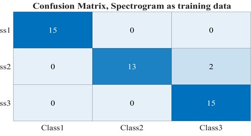
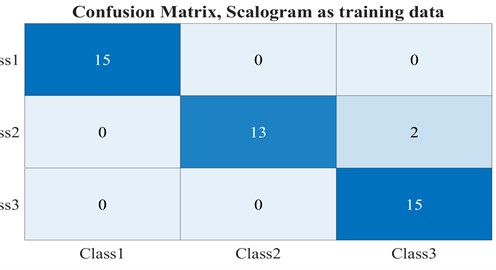
After training and then testing the CNNs-based network for spectrogram and scalogram figures as input, in the testing step, both trained networks revealed the same accuracy, 95.5 %. Fig. 8 shows the confusion matrices as the results of the testing steps.
To have an analysis, from the above figures, both networks could recognize cracked rotors from healthy ones, among 45 samples as the testing stage, the 30 cracked ones have distinguished properly, but two samples belonged to Class 2, cracked rotor with 0.32, have classified as Class 3. This mistake can be stem from the fact that since some samples were obtained in the low initial accelerations and a system with low density in the shaft, the Scalogram and Spectrogram of these situations are similar to high initial acceleration and high-density plots. On the whole, the quality of images plays an important role in CNNs. The main benefit of this procedure is that in many current processes in the classification, such as artificial neural network, Support vector machine, -nearest neighbors (-NN) algorithm, and other methods like these areas, feature extraction, and feature selection are considered as the significant stages in the method effectiveness. Although this procedure can be heavy in the calculation, the graphics processing unit (GPU) can solve this issue; the default feature extraction method from images can result in a rational accuracy, 95.5 %.
Fig. 8Confusion matrices for the networks with a) spectrogram, b) scalogram figures as input
a)
b)
5. Conclusions
In this study, by applying Deep learning procedure rotor-bearing-disc is classified based on its healthy condition. To begin, the system is modeled employing the finite element method, and its mass, stiffness, damping, and force matrices are extracted; crack in the system is modeled by applying strain energy procedure and extra flexibility of the crack is added to the element that contains a crack. After assembling the local matrices and creating global matrices, the system’s equation of motion is solved by employing the numerical Houbolt time-marching method and the vibration signals are calculated during the system’s start-up and for several conditions, i.e. 300 samples. As the pre-process procedure, Continuous Wavelet transform and Short-time Fourier transform are exerted to the signals and the related figures are saved as the training data to the Deep Learning process. AlexNet network with 25 layers based on convolutional neural networks is applied as the used network. By training 85 percent of the data as the training process and 15 percent of the data as the testing stage, the results of the trained network are shown in the form of confusion matrices. The reasonable accuracy of the trained network, i.e. 95.5 percent approves that the trained network in both Scalogram and Spectrogram based input data has a great capacity in the classification of cracked rotors. For future studies, a test rig can be designed and the real datasets can verify the accuracy of the trained network.
References
-
Nima Rezazadeh, “Investigation on the time-frequency effects of a crack in a rotating system,” International Journal of Engineering Research and Technology, Vol. 9, No. 6, Jul. 2020.
-
A. S. Sekhar and B. S. Prabhu, “Condition monitoring of cracked rotors through transient response,” Mechanism and Machine Theory, Vol. 33, No. 8, pp. 1167–1175, Nov. 1998, https://doi.org/10.1016/s0094-114x(97)00116-x
-
N. H. Chandra and A. S. Sekhar, “Fault detection in rotor bearing systems using time frequency techniques,” Mechanical Systems and Signal Processing, Vol. 72-73, pp. 105–133, May 2016, https://doi.org/10.1016/j.ymssp.2015.11.013
-
D. Söffker, C. Wei, S. Wolff, and M.-S. Saadawia, “Detection of rotor cracks: comparison of an old model-based approach with a new signal-based approach,” Nonlinear Dynamics, Vol. 83, No. 3, pp. 1153–1170, Feb. 2016, https://doi.org/10.1007/s11071-015-2394-5
-
M. J. Gómez, C. Castejón, and J. C. García-Prada, “Crack detection in rotating shafts based on 3× energy: Analytical and experimental analyses,” Mechanism and Machine Theory, Vol. 96, No. 1, pp. 94–106, Feb. 2016, https://doi.org/10.1016/j.mechmachtheory.2015.09.009
-
W. Zhao, C. Hua, D. Dong, and H. Ouyang, “A novel method for identifying crack and shaft misalignment faults in rotor systems under noisy environments based on CNN,” Sensors, Vol. 19, No. 23, p. 5158, Nov. 2019, https://doi.org/10.3390/s19235158
-
B. A. Shah and D. P. Vakharia, “Testing for detection of crack in rotor using vibration analysis: an experimental approach,” International Journal of Quality and Reliability Management, Vol. 36, No. 6, pp. 999–1013, Jun. 2019, https://doi.org/10.1108/ijqrm-06-2017-0107
-
R. Nima and F. Shila, “Crack classification in rotor-bearing system by means of wavelet transform and deep learning methods: an experimental investigation,” Journal of Mechanical Engineering, Automation and Control Systems, Vol. 1, No. 2, pp. 102–113, Dec. 2020, https://doi.org/10.21595/jmeacs.2020.21799
-
P. Sathujoda, “Detection of a slant crack in a rotor bearing system during shut-down,” Mechanics Based Design of Structures and Machines, Vol. 48, No. 2, pp. 266–276, Mar. 2020, https://doi.org/10.1080/15397734.2019.1707686
-
N. Kushwaha and V. N. Patel, “Modelling and analysis of a cracked rotor: a review of the literature and its implications,” Archive of Applied Mechanics, Vol. 90, No. 6, pp. 1215–1245, Jun. 2020, https://doi.org/10.1007/s00419-020-01667-6
-
H. D. Nelson and J. M. Mcvaugh, “The dynamics of rotor-bearing systems using finite elements,” Journal of Engineering for Industry, Vol. 98, No. 2, pp. 593–600, May 1976, https://doi.org/10.1115/1.3438942
-
C. A. Papadopoulos and A. D. Dimarogonas, “Coupled longitudinal and bending vibrations of a rotating shaft with an open crack,” Journal of Sound and Vibration, Vol. 117, No. 1, pp. 81–93, Aug. 1987, https://doi.org/10.1016/0022-460x(87)90437-8
-
H. Tada, P. C. Paris, and G. R. Irwin, The Stress Analysis of Cracks Handbook, Third Edition. ASME Press, 2000, https://doi.org/10.1115/1.801535
-
A. S. Sekhar and P. Balaji Prasad, “Dynamic analysis of a rotor system considering a slant crack in the shaft,” Journal of Sound and Vibration, Vol. 208, No. 3, pp. 457–474, Dec. 1997, https://doi.org/10.1006/jsvi.1997.1222
-
C. A. Papadopoulos, “Some comments on the calculation of the local flexibility of cracked shafts,” Journal of Sound and Vibration, Vol. 278, No. 4-5, pp. 1205–1211, Dec. 2004, https://doi.org/10.1016/j.jsv.2003.12.023
-
C. A. Papadopoulos and A. D. Dimarogonas, “Stability of cracked rotors in the coupled vibration mode,” Journal of Vibration and Acoustics, Vol. 110, No. 3, pp. 356–359, Jul. 1988, https://doi.org/10.1115/1.3269525
-
A. K. Darpe, K. Gupta, and A. Chawla, “Coupled bending, longitudinal and torsional vibrations of a cracked rotor,” Journal of Sound and Vibration, Vol. 269, No. 1-2, pp. 33–60, Jan. 2004, https://doi.org/10.1016/s0022-460x(03)00003-8
-
M. Hossain and H. Wu, “Crack breathing behavior of unbalanced rotor system: A Quasi-static numerical analysis,” Journal of Vibroengineering, Vol. 20, No. 3, pp. 1459–1469, May 2018, https://doi.org/10.21595/jve.2018.19692
-
P. Kim, MATLAB Deep Learning. Berkeley, CA: APress, 2017, https://doi.org/10.1007/978-1-4842-2845-6
-
Dan Claudiu Ciresan et al., “Flexible, high performance convolutional neural networks for image classification,” in Proceedings of the 22nd International Joint Conference on Artificial Intelligence, pp. 1237–1242, Jul. 2011, https://doi.org/10.5591/978-1-57735-516-8/ijcai11-210
-
D. Sundararajan, Discrete wavelet Transform. Singapore: John Wiley & Sons, Singapore Pte. Ltd, 2015, p. 2015, https://doi.org/10.1002/9781119113119
-
J. Allen, “Short term spectral analysis, synthesis, and modification by discrete Fourier transform,” IEEE Transactions on Acoustics, Speech, and Signal Processing, Vol. 25, No. 3, pp. 235–238, Jun. 1977, https://doi.org/10.1109/tassp.1977.1162950
Cited by
About this article

