Abstract
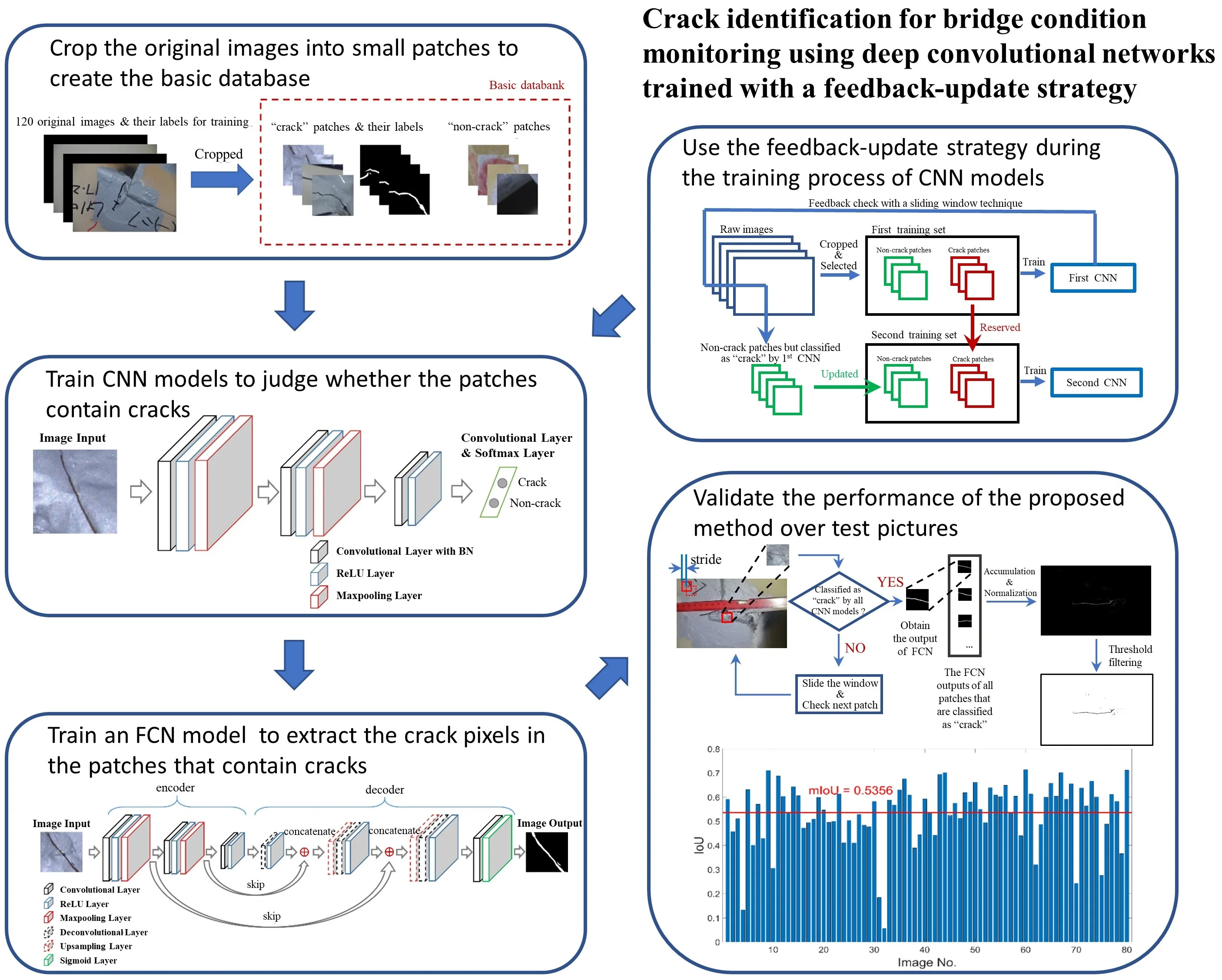
Orthotropic steel bridge decks and steel box girders are key structures of long-span bridges. Fatigue cracks often occur in these structures due to coupled factors of initial material flaws and dynamic vehicle loads, which drives the need for automating crack identification for bridge condition monitoring. With the use of unmanned aerial vehicle (UAV), the acquirement of bridge surface pictures is convenient, which facilitates the development of vision-based bridge condition monitoring. In this study, a combination of convolutional neural network (CNN) with fully convolutional network (FCN) is designed for crack identification and bridge condition monitoring. Firstly, 120 images are cropped into small patches to create a basic dataset. Subsequently, CNN and FCN models are trained for patch classification and pixel-level crack segmentation, respectively. In patch classification, some non-crack patches that contain complicated disturbance information, such as handwriting and shadow, are often mistakenly identified as cracks by directly using the CNN model. To address this problem, we propose a feedback-update strategy for CNN training, in which mistaken classification results of non-crack data are selected to update the training set to generate a new CNN model. By that analogy, several different CNN models are obtained and the accuracy of patch classification could be improved by using all models together. Finally, 80 test images are processed by the feedback-update CNN models and FCN model with a sliding window technique to generate crack identification results. Intersection over union (IoU) is calculated as an index to quantificationally evaluate the accuracy of the proposed method.
Highlights
- A pixel-level crack identification method with a combination of convolutional neural networks (CNNs) and fully convolutional networks (FCNs) is proposed.
- Feedback-update strategy is proposed, which updates and optimizes the training set during the CNN training process. This strategy can improve the performance of CNN model significantly.
- The crack identification results over 80 test images demonstrate the effectiveness of the proposed method and the feedback-update strategy.
1. Introduction
The steel box girder is extensively used in long span bridges, which suffer from fatigue cracks under dynamic loads owing to initial flaws in the welding joints and connections. The development and expansion of cracks will decrease the structural reliability and shorten the operational life span of bridges [1]. To ensure safety, there is enormous interest in the research of bridge condition monitoring methods to detect fatigue cracks automatically. Due to the rapid development of computer vision, vision-based condition monitoring methods have become a research focus. In addition, with the help of UAVs and bridge robots, numerous pictures of bridge surface are convenient to collect, which guarantees the feasibility of vision-based monitoring.
Various vision-based methods based on conventional digital image processing techniques (IPTs) for detecting cracks have been proposed and investigated in the civil engineering field. Abdel-Qader et al. [2] provided a comparison of four crack-detection techniques: fast Haar transform (FHT), fast Fourier transform, Sobel edge detector, and Canny edge detector. The result shows that FHT is more reliable than the other three edge-detection techniques in identifying cracks in the bridge. Yamaguchi and Hashimoto [3] introduced an efficient and high-speed crack detection method that employs percolation-based image processing. Zou et al. [4] developed a fully-automatic method called CrackTree to detect cracks from pavement images. Yeum and Dyke [5] proposed research for detecting cracks near bolts using IPTs with prior knowledge. Li et al. [6] developed a method to detect concrete cracks with a local binarization algorithm. However, the results of IPTs are sensitive to the environmental variety of the real-world situations, which limits the detection accuracy.
Recently, deep learning techniques have been developed for image-based crack detection in computer vision. As one of the most representative and effective deep learning methods, deep convolutional neural networks (CNNs) are extensively used in cracks identification. Modarres et al. [7] concluded that CNN is an effective tool for the crack detection compared with several other machine learning algorithms. Cha et al. [8] used CNNs combined with a sliding window technique to design an effective classifier to detect cracks in relatively large images. Wang et al. [9] proposed a CNN model consisting of 3 convolution layers and 2 fully-connected layers for recognizing cracks on asphalt surfaces at subdivided image cell. Zhang et al. [10] trained a supervised deep convolutional neural network to identify pavement cracks in the collected images. Gopalakrishnan et al. [11] employed a deep convolutional neural network (DCNN) and transferred that learning to automatically detect cracks in pavement images that also include a variety of non-crack anomalies and defects. Yao et al. [12] improved the traditional convolution network structure by adding the inception modules, which enhanced the robustness of the DCNN model for detecting bugholes on concrete surfaces. Xu et al. [13] proposed a modified fusion convolutional neural network architecture to identify cracks from real-world images containing complicated disturbance information inside steel box girders of bridges. Kim et al. [14] applied mask and region-based convolutional neural network (Mask R-CNN) to execute the preliminary identification of concrete cracks. Wei et al. [15] modified the architecture of the Mask R-CNN to quantify defects of concrete surface. Although CNN-based crack image classification and detection techniques have shown robust performance compared with conventional IPTs, these image-level methods do not provide precise information about the crack shape and other details. Therefore, it is of significance to develop a pixel-level crack segmentation method to extract elaborate features of cracks in an image.
In recent years, pixel-level semantic segmentation in computer vision has developed rapidly stimulated by the convolution technique. Long et al. [16] proposed fully convolutional networks (FCNs), which achieve encouraging performance in the field of computer vision-based semantic segmentation, such as for scene parsing or biomedical image segmentation. Inspired by the appearance of FCNs, several researchers have applied FCNs or improved FCNs to crack segmentation. Dung et al. [17] proposed a crack detection method based on deep FCN for semantic segmentation on concrete crack images. Islam et al. [18] applied an FCN-based autonomous crack detection method to accurately detect cracks. Ren et al. [19] proposed an improved deep fully convolutional neural network, named CrackSegNet, to conduct dense pixel-wise crack segmentation. Yang et al. [20] proposed a feature pyramid and hierarchical boosting network (FPHBN) to automatically detect crack in an end-to-end way, which adopts the idea of holistically-nested edge detection (HED) [21], a breakthrough edge detection method inspired by fully convolutional neural networks. Sun et al. [22] implemented a deep learning technique based on DeepLabv3+ to detect cracks and bugholes on concrete surfaces at the pixel level. These FCN-based methods make it possible to conduct pixel-wise crack segmentation, which could provide precise information and high-level features of cracks in an image.
In this paper, a crack identification method with a combination of CNN and FCN is proposed. Firstly, we use CNNs with a sliding window technique in a relatively large image to search for the small patches that contain cracks. Subsequently, an FCN model is applied to achieve cracks identification at the pixel level. Former researchers pay more attention to the improvement of the network architecture to achieve better performance, while the optimization of the training data is usually short of focus. However, the construction of training set has a significant effect on the capability of the network. The background of the crack images on the steel box girder is complex, and some complicated disturbance information, such as handwriting, spots, shadow, and welding line, is often identified as crack by the CNN. Thus, it is particularly important to construct an abundant and complete training set. Here, we propose a novel strategy in the process of training data construction and network training. Original images are cropped into some small patches labeled as “crack” or “non-crack” to train a classification CNN. Then, the CNN is applied back to the original images with a sliding window to search for the patches of misclassification. Next, these misclassification patches are used to train a new CNN. By that analogy, several different CNNs are acquired for crack classification. The cracks identification results are more distinct and precise compared with the situation in which a single CNN is used.
The rest of this paper is organized as follows. The introduction of CNN, FCN, the proposed training strategy, and overall procedure for crack identification is given in Section 2. The experimental results, including model training and accuracy analysis, are presented in Section 3. The influence of the feedback-update strategy and the stride is explored in Section 4. Finally, conclusions are drawn in Section 5.
2. Methodology
2.1. Convolutional neural network
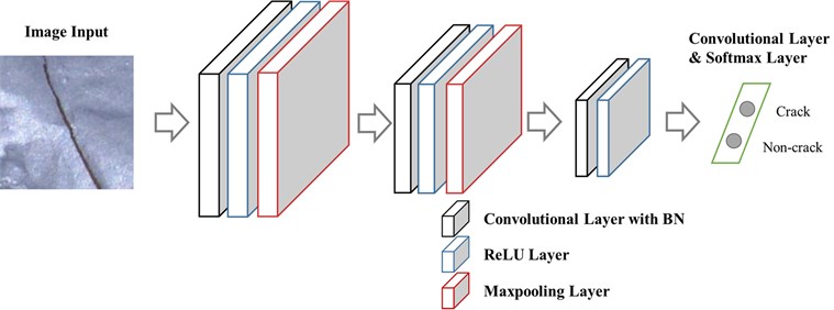
A CNN architecture consists of several convolutional blocks. Each convolutional block is composed of a convolutional layer, an activation unit, and a pooling layer. A deep CNN is defined when the architecture is composed of many layers. Some other auxiliary layers, such as dropout and batch normalization (BN) layers, can be implemented within the aforementioned layers in accordance with the purposes of use. Fig. 1 shows the CNN architecture used in this study for crack classification. The input layer is the labeled image patch of 224×224×3 pixel resolutions, where each dimension means height, width, and depth (RBG), respectively. Table 1 lists the details of each layer and operation.
Fig. 1Network architecture of CNN for patch classification
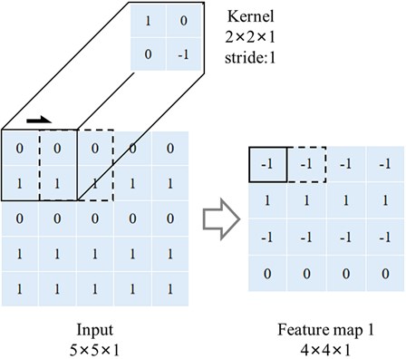
The main objective of convolutional layer is feature extraction. First, the dot product between a 2D array named convolutional kernel or filter and a sub-array of an input image patch at a certain location is calculated. The size of a sub-array is always equal to the convolutional kernel, but a convolutional kernel is always smaller than the input image. Second, the bias is added to the value. Next, the convolutional kernel slides across the input image’s width and height with a distance named stride and the dot production added with bias is calculated again. After the whole input image is scanned, the values at different positions constitute a feature map. One convolutional layer could have several kernels, and the number of the convolutional kernels determines the depth of the feature map. An operation example of a convolutional layer is shown in Fig. 2.
Table 1Dimensions of layers and operations
Layer | Height | Width | Depth | Operator | Kernel size | Numbers | Stride |
Input | 224 | 224 | 3 | Convolution | 20 × 20 | 24 | 2 |
L1 | 103 | 103 | 24 | ReLU | – | – | – |
L2 | 103 | 103 | 24 | Max-pooling | 7 × 7 | – | 2 |
L3 | 49 | 49 | 24 | Convolution | 15 × 15 | 48 | 2 |
L4 | 18 | 18 | 48 | ReLU | – | – | – |
L5 | 18 | 18 | 48 | Max-pooling | 4 × 4 | – | 2 |
L6 | 8 | 8 | 48 | Convolution | 8 × 8 | 96 | 1 |
L7 | 1 | 1 | 96 | ReLU | – | – | – |
L8 | 1 | 1 | 96 | Convolution | 1 × 1 | 2 | 1 |
L9 | 1 | 1 | 2 | Softmax | – | – | – |
L10 | 1 | 1 | 2 | – | – | – | – |
Fig. 2Network architecture of CNN for patch classification
An activation function follows the convolution process to introduce nonlinearity to the model. Various activation functions such as sigmoid or tanh can be used, but the rectified linear unit (ReLU) [23] is preferred in most situations, as it can train the network much faster than the other activation functions. After the ReLU operation, all the negative values are transformed to zero. The ReLU activation function is defined as follows:
The pooling layer is used to reduce the spatial size of the feature map after convolution and activation, which reduces overfitting and the training time. There are two different pooling options. The max-pooling layer takes the maximum value of each pooling kernel, and average pooling layer takes the average value of each pooling kernel from the prior feature map [24]. In this study, the max-pooling layer is used.
Some auxiliary layers can assist in the model training. Dropout layer [25] is a trick to reduce overfitting. The thought of dropout is to randomly interrupt the connections between neurons of connected layers with a pre-set dropout rate when training. Batch normalization [26] is also a well-known trick for network training, which facilitates high-learning rate and leads to much faster network convergence.
2.2. Feedback-update strategy for training data optimization of CNN
In an original image, the information of the background is complex. In practice, the area of cracks could be identified effectively while other areas that contain handwriting, welding line, spots, or shadow are often mistakenly identified as crack area when using CNN with a sliding window over a test image. Therefore, it is necessary to find a solution to classify these fake-crack features more precisely.
Fig. 3The feedback-update strategy of CNNs training and dataset updating
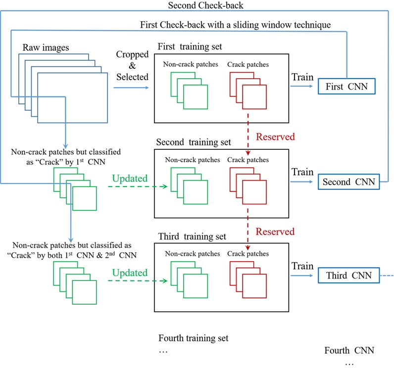
To address this problem, a simple but effective strategy named “feedback-update” is proposed. First, part of labeled patches cropped from original pictures are used to train the first CNN model. Subsequently, the first CNN model is applied back to the original pictures with a sliding window to collect the non-crack patches which are mistakenly identified as crack area. Next, the patches labeled “crack” in the original training set remain unchanged while the patches labeled “non-crack” are replaced by the new collected patches, and the second CNN model is trained with the new training set. Similarly, the patches that do not contain cracks but are identified as crack area by both CNN models can be collected for training the third CNN. By that analogy, several different CNN models for classification are acquired. Only the patches that are identified as crack area by all CNN models would be treated as crack area for sematic segmentation by FCN in the next procedure. The whole flow chart of CNNs training is shown as Fig. 3.
2.3. Fully convolutional network
The input layer of the FCN is the same as that of the aforementioned CNN and the output layer is a grey-scale image of 224×224 pixel resolutions which contains pixel-level information of cracks. Network architecture of FCN model mainly consists of an encoder and a decoder, which is shown in Fig. 4. The encoder contains several convolutional and pooling layers, which is used to extract features necessary for semantic segmentation. The weights of the CNN trained for crack classification are used for initialization of the encoder. The decoder uses deconvolution (transpose convolution) and up-sampling layers to reconstruct the corresponding segmented image. Each deconvolution layer of the decoder matches a corresponding convolution layer of the encoder and each up-sampling layer of the decoder matches a corresponding pooling layer of the encoder. There are many techniques for up-sampling, such as bilinear and nearest. In this study, bilinear is used for up-sampling.
Fig. 4Network architecture of FCN for sematic segmentation
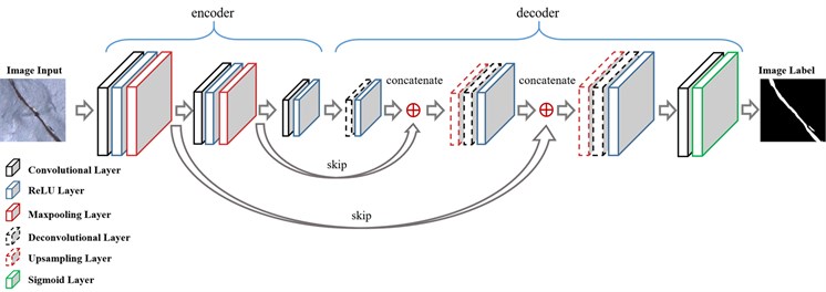
Adding skips [27] adopted by Long et al. is a trick for a more precise segmentation. In the decoding process, the output of each deconvolutional layer in the decoder is concatenated with output of the corresponding pooling layer in the encoder. Combining fine layers and coarse layers lets the model make local predictions that respect global structure [16].
The last step of FCN is a sigmoid function, which restricts the values of the pixels in the output image to a range between 0 and 1. The closer that the value of a pixel is to 1, the more likely the cracks cross through the location of this pixel in the image. The sigmoid activation function is defined as:
2.4. Overall procedure for crack identification
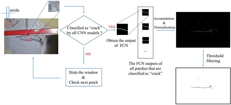
Through the aforementioned procedure, several CNN models for patch classification and an FCN model for sematic segmentation are obtained. These networks can be used for cracks identification at the pixel level with a sliding window technique. The whole procedure is shown in Fig. 5.
A rectangular window slides over the test image and the image patch in the window is judged by the CNNs. If all the CNN models classify the patch as “crack”, the patch will be treated as the input for the FCN to obtain the segmentation result of the small area within the sliding window. It is worth mentioning that a pixel would be enclosed by more than one window, so one pixel may have several segmentation values under different windows. After the window slides over the whole test image, the segmentation values of each pixel are added up at the corresponding locations on the image. Through such a process of accumulation, the information of cracks could be reinforced and some disturbance identified as crack by accident could be suppressed. Then, the pixel values of the image are normalized to a range between 0 and 1. The closer a pixel value is to 1, the more likely the location of the pixel on the image belongs to crack. At this point, the segmentation result is fuzzy since the segmentation values of the pixels are continuous. Therefore, a threshold is set, and all the pixels whose segmentation values are larger than the threshold constitute the crack area (shown in black), by which each pixel is classified into “crack” or “non-crack” classes.
Fig. 5The procedure for crack identification using CNN & FCN models with a sliding window
3. Case study
3.1. Dataset introduction
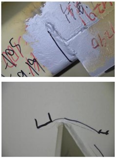
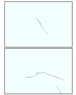
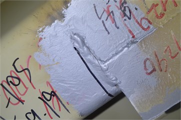
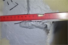
Orthotropic steel bridge decks and steel box girders are key structures of long-span bridges. Due to coupled factors of initial material flaws and dynamic vehicle loads, cracks often occur at the bridge connection details, especially around welding joints. The images of the dataset are obtained by different bridge inspectors and captured with a variety of internal and external camera parameters. The dataset includes two folders: Images (*.PNG) and Labels (*.PNG) as shown in Fig. 6. The Images folder includes 120 original fatigue crack images with resolutions of 4928×3264 and 5152×3864. Except for 120 image-label pairs for training process, 80 additional original images with resolutions of 4928×3264 are also used to validate the performance of the model.
Fig. 6Examples of the steel box girder fatigue crack image dataset: a) original fatigue crack image and b) pixel-level binary ground-truth label
a)
b)
The 120 raw images and their labels are cropped into small patches of 224×224 pixel resolutions to build basic databank for model training, which is shown in Fig. 7. Because the crack area is much smaller than non-crack area in the raw images, the number of the cropped patches with cracks is much less than that of patches without cracks. To address this imbalance, the original crack patches are processed by rotation. As shown in Fig. 8, the rotation angles are 0°, 45°, 90°, 135°, 180°, 225°, 270°, and 315°, respectively. By this operation, the number of crack patches is expanded to 8 times.
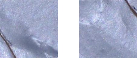
Some cropped images are with cracks on the four edges, which is shown in Fig. 9. These types of patches are removed from training databank for the following reasons. Firstly, the characteristics of such image patches for training are not representative, which may lead to the misclassification of testing. Secondly, cracks located in any positions of the test image spaces can cross the center of the sliding window if a relatively small stride is set. That is, ignoring the patches with cracks on the edges does not lead to information omission.
Fig. 7The establishment of the basic databank
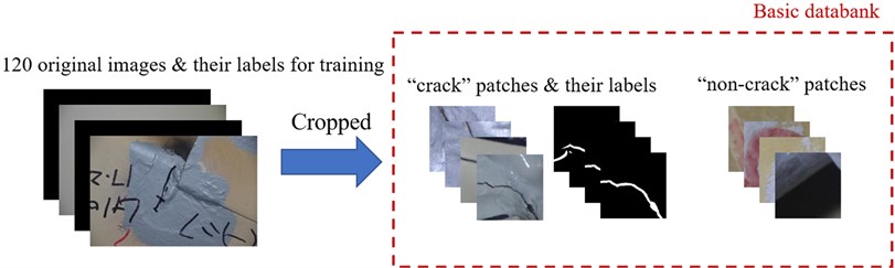
Fig. 8Illustration of data augmentation
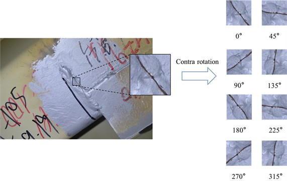
Fig. 9Cropped patches with cracks on the edges
3.2. Model training
According to the feedback-update strategy, a series of CNN models could be trained for patch classification. In this case, two CNN models are trained.
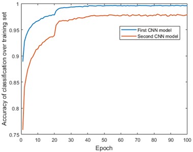
16000 image patches labeled “crack” and 16000 image patches labeled “non-crack” are randomly chosen from databank to construct the training set for the first CNN model. The CNN is trained for 100 epochs with a batch size of 32. The learning rate changes as epoch grows (Table 2). The training process of the first CNN model is shown in Fig. 10(a).
Fig. 10The training process: a) CNN models and b) FCN model
a)
b)
Fig. 11Patch classification of the first CNN: a) an example from 120 original images for training and b) patches that are classified as “crack” by the first CNN
a)
b)
The first CNN is applied back to the 120 raw images with a 30-stride sliding window. The patch-classification result of an image is shown in Fig. 11. Obviously, some non-crack patches are classified as “crack”, which indicates the necessity of training the second CNN model. 31352 non-crack patches of the 120 images are classified as “crack” by mistake in total. 4000 patches are selected from them and augmented to 16000 by rotation, which is used to create a new training set together with the 16000 image patches labeled “crack” in the original training set. Subsequently, the second CNN model is trained with the same hyperparameters of the first CNN. The training process of the second CNN is also shown in Fig. 10(a).
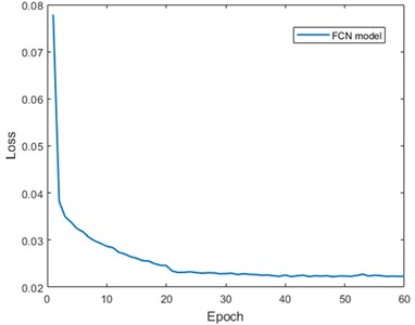
After CNNs, 462 image patches labeled “crack” and the labels are selected from the databank to build the training set for the FCN model. The training set is shown in Fig. 12. The FCN is trained for 60 epochs with a batch size of 4. The learning rate and training process are shown in Table 2 and Fig. 10(b), respectively.
Fig. 12Patch classification of the first CNN: a) an example from 120 original images for training and b) patches that are classified as “crack” by the first CNN
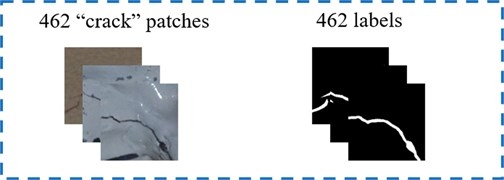
Table 2Learning rate
Epoch | CNN | FCN |
1-20 | 0.01 | 0.01 |
21-40 | 0.001 | 0.001 |
41-60 | 0.0001 | 0.0001 |
61-80 | 0.00001 | – |
81-100 | 0.000001 | – |
3.3. Evaluation of the result
Several metrics can be used for accuracy evaluation, including pixel accuracy (PA), intersection over union (IoU), precision, recall, and F1 score [19]. In this case, IoU is adopted as an index for segmentation evaluation. The accuracy of crack identification is better with a larger IoU. For binary classification, IoU is defined as:
where TP, FP and FN represent the pixel number of true positives, false positives and false negatives, respectively.
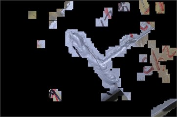
Fig. 13An example of test results (IoU = 0.5915): a) original test image, b) patches that are classified as “crack” by CNNs (shown in white), c) fuzzy result before threshold filtering, d) final result of sematic segmentation and e) ground truth
a)
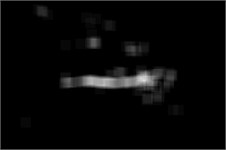
b)
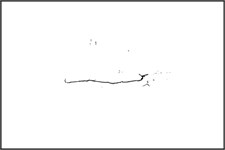
d)

c)
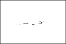
e)
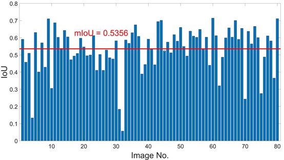
80 raw images that are not used in the training process are used for tests. The ground truth of the 80 images is acquired by Photoshop. The test procedure is described in Section 2.4. The threshold used in the filtering is set at 0.2. If the normalized value of a pixel is larger than 0.2, the pixel will be classified as crack pixel. An example of test results is shown in Fig. 13. As can be seen, although there are a few non-crack pixels that are classified as crack area, the main part of the crack is identified distinctly. The IoU of 80 test images is shown in Fig. 14 and the mean IoU (mIoU) is 0.5356.
Fig. 14The IoU of 80 test images
4. Discussions
4.1. Comparison of crack detection accuracy between the models with two CNNs and one CNN
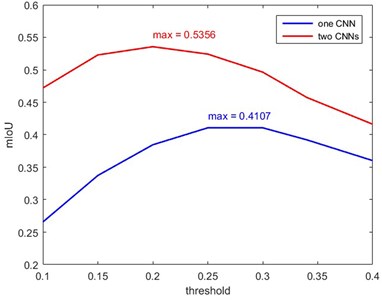
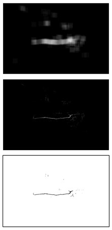
For comparison, only the first CNN model is used to execute the patch classification. A comparison example between the segmentation results of the models with two CNNs and one CNN is shown in Fig. 15. Obviously, the crack identification result of the model with two CNNs is clearer than that with one CNN. The IoU of both strategies over 80 test images is calculated and compared with each other in Fig. 16. As can be seen, the mIoU of the model with two CNNs is larger at any threshold value, which demonstrates a high crack-detection capability of the proposed method.
Fig. 15The results of different models: a) test image and ground truth, b) segmentation result of the model with two CNNs and c) segmentation result of the model with a single CNN

a)

b)
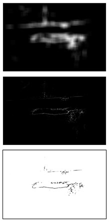
c)
Fig. 16Comparison of the mIoU under different threshold values
4.2. The influence of the stride
In this study, CNN and FCN are applied to the test image with a sliding window technique. The stride of the sliding window is set at 30. The influence of stride variety on the crack identification result is investigated here.
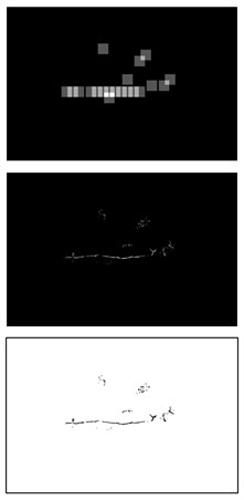
Fig. 17The influence of the stride: a) test image and ground truth, b) stride = 30 and c) stride = 130
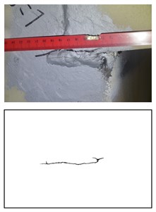
a)
b)
c)
Fig. 17 shows the comparison of results with stride 30 and 130. As can be seen, the result with stride 30 is smoother and clearer than that with stride 130. Therefore, it can be inferred that adopting a small stride in a reasonable range can highlight the main part of the crack and suppress the noise. However, a smaller stride may lead to information loss of the crack ends and more operating time of testing.
5. Conclusions
In this study, a vision-based method of fatigue crack identification for bridge condition monitoring is proposed. Compared with the previous research, the innovations of the method presented in this paper are concluded as follows.
1) A method for crack identification with a combination of CNN and FCN is proposed. CNN and FCN are the two deep learning models widely used for crack detection. In order to take advantage of both models, we combine CNN with FCN during crack detection. 20 images with resolutions of 4928×3264 and 5152×3864 are cropped into small image patches with 224×224 pixel resolutions for training process. The performance of the proposed method is evaluated on 80 test images with resolutions of 4928×3264 pixels. The test images are scanned by the trained CNN models with a sliding window technique, which facilitates the scanning of any images larger than 224×224 pixel resolutions, and the patches classified as “crack” are input into the FCN model to obtain pixel-level segmentation results. After normalization and filtering, the final crack identification results are acquired and evaluated by IoU. The mIoU over 80 test images is 0.5356.
2) The feedback-update strategy is proposed for dataset optimization, which improves the performance of the CNN models for crack identification. In the training process of CNN model, we notice that handwriting, welding line, spots and shadow are often mistakenly identified as crack area. To address this problem, the feedback-update strategy is presented. The first trained CNN model is applied back to the 120 raw images to collect the non-crack patches which are classified as “crack” by mistake. Then the collected patches are used to replace and update the “non-crack” data in the original training set. Subsequently, the new training set is used to train the second CNN model. By that analogy, several CNN models can be generated for patch classification. In practice, the method performance with two CNN models is improved, and mIoU of the method is much larger than that of the model with a single CNN.
References
-
S. Ya, K. Yamada, and T. Ishikawa, “Fatigue evaluation of rib-to-deck welded joints of orthotropic steel bridge deck,” Journal of Bridge Engineering, Vol. 16, No. 4, pp. 492–499, Jul. 2011, https://doi.org/10.1061/(asce)be.1943-5592.0000181
-
I. Abdel-Qader, O. Abudayyeh, and M. E. Kelly, “Analysis of edge-detection techniques for crack identification in bridges,” Journal of Computing in Civil Engineering, Vol. 17, No. 4, pp. 255–263, Oct. 2003, https://doi.org/10.1061/(asce)0887-3801(2003)17:4(255)
-
T. Yamaguchi and S. Hashimoto, “Fast crack detection method for large-size concrete surface images using percolation-based image processing,” Machine Vision and Applications, Vol. 21, No. 5, pp. 797–809, Aug. 2010, https://doi.org/10.1007/s00138-009-0189-8
-
Q. Zou, Y. Cao, Q. Li, Q. Mao, and S. Wang, “CrackTree: Automatic crack detection from pavement images,” Pattern Recognition Letters, Vol. 33, No. 3, pp. 227–238, Feb. 2012, https://doi.org/10.1016/j.patrec.2011.11.004
-
C. M. Yeum and S. J. Dyke, “Vision-based automated crack detection for bridge inspection,” Computer-Aided Civil and Infrastructure Engineering, Vol. 30, No. 10, pp. 759–770, Oct. 2015, https://doi.org/10.1111/mice.12141
-
L. Li, Q. Wang, G. Zhang, L. Shi, J. Dong, and P. Jia, “A method of detecting the cracks of concrete undergo high-temperature,” Construction and Building Materials, Vol. 162, pp. 345–358, Feb. 2018, https://doi.org/10.1016/j.conbuildmat.2017.12.010
-
C. Modarres, N. Astorga, E. L. Droguett, and V. Meruane, “Convolutional neural networks for automated damage recognition and damage type identification,” Structural Control and Health Monitoring, Vol. 25, No. 10, p. e2230, Oct. 2018, https://doi.org/10.1002/stc.2230
-
Y.-J. Cha, W. Choi, and O. Büyüköztürk, “Deep learning-based crack damage detection using convolutional neural networks,” Computer-Aided Civil and Infrastructure Engineering, Vol. 32, No. 5, pp. 361–378, May 2017, https://doi.org/10.1111/mice.12263
-
K. C. P. Wang, A. Zhang, J. Q. Li, Y. Fei, C. Chen, and B. Li, “Deep learning for asphalt pavement cracking recognition using convolutional neural network,” in International Conference on Highway Pavements and Airfield Technology 2017, pp. 166–177, Aug. 2017, https://doi.org/10.1061/9780784480922.015
-
L. Zhang, F. Yang, Y. Daniel Zhang, and Y. J. Zhu, “Road crack detection using deep convolutional neural network,” in 2016 IEEE International Conference on Image Processing (ICIP), pp. 3708–3712, Sep. 2016, https://doi.org/10.1109/icip.2016.7533052
-
K. Gopalakrishnan, S. K. Khaitan, A. Choudhary, and A. Agrawal, “Deep convolutional neural networks with transfer learning for computer vision-based data-driven pavement distress detection,” Construction and Building Materials, Vol. 157, pp. 322–330, Dec. 2017, https://doi.org/10.1016/j.conbuildmat.2017.09.110
-
G. Yao, F. Wei, Y. Yang, and Y. Sun, “Deep-learning-based bughole detection for concrete surface image,” Advances in Civil Engineering, Vol. 2019, pp. 1–12, Jun. 2019, https://doi.org/10.1155/2019/8582963
-
Y. Xu, Y. Bao, J. Chen, W. Zuo, and H. Li, “Surface fatigue crack identification in steel box girder of bridges by a deep fusion convolutional neural network based on consumer-grade camera images,” Structural Health Monitoring, Vol. 18, No. 3, pp. 653–674, May 2019, https://doi.org/10.1177/1475921718764873
-
B. Kim and S. Cho, “Image‐based concrete crack assessment using mask and region‐based convolutional neural network,” Structural Control and Health Monitoring, Vol. 26, No. 8, p. e2381, Jun. 2019, https://doi.org/10.1002/stc.2381
-
F. Wei, G. Yao, Y. Yang, and Y. Sun, “Instance-level recognition and quantification for concrete surface bughole based on deep learning,” Automation in Construction, Vol. 107, p. 102920, Nov. 2019, https://doi.org/10.1016/j.autcon.2019.102920
-
J. Long, E. Shelhamer, and T. Darrell, “Fully convolutional networks for semantic segmentation,” in 2015 IEEE Conference on Computer Vision and Pattern Recognition (CVPR), pp. 3431–3440, Jun. 2015, https://doi.org/10.1109/cvpr.2015.7298965
-
C. V. Dung and L. D. Anh, “Autonomous concrete crack detection using deep fully convolutional neural network,” Automation in Construction, Vol. 99, pp. 52–58, Mar. 2019, https://doi.org/10.1016/j.autcon.2018.11.028
-
M. M. M. Islam and J.-M. Kim, “Vision-based autonomous crack detection of concrete structures using a fully convolutional encoder-decoder network,” Sensors, Vol. 19, No. 19, p. 4251, Sep. 2019, https://doi.org/10.3390/s19194251
-
Y. Ren et al., “Image-based concrete crack detection in tunnels using deep fully convolutional networks,” Construction and Building Materials, Vol. 234, p. 117367, Feb. 2020, https://doi.org/10.1016/j.conbuildmat.2019.117367
-
F. Yang, L. Zhang, S. Yu, D. Prokhorov, X. Mei, and H. Ling, “Feature pyramid and hierarchical boosting network for pavement crack detection,” IEEE Transactions on Intelligent Transportation Systems, Vol. 21, No. 4, pp. 1525–1535, Apr. 2020, https://doi.org/10.1109/tits.2019.2910595
-
S. Xie and Z. Tu, “Holistically-nested edge detection,” in 2015 IEEE International Conference on Computer Vision (ICCV), pp. 1395–1403, Dec. 2015, https://doi.org/10.1109/iccv.2015.164
-
Y. Sun, Y. Yang, G. Yao, F. Wei, and M. Wong, “Autonomous crack and bughole detection for concrete surface image based on deep learning,” IEEE Access, Vol. 9, pp. 85709–85720, 2021, https://doi.org/10.1109/access.2021.3088292
-
V. Nair and G. E. Hinton, “Rectified linear units improve restricted Boltzmann machines,” in Proceedings of the 27th International Conference on Machine Learning, pp. 807–814, 2010.
-
D. Scherer, A. Müller, and S. Behnke, “Evaluation of pooling operations in convolutional architectures for object recognition,” in Artificial Neural Networks – ICANN 2010, Berlin, Heidelberg: Springer Berlin Heidelberg, 2010, pp. 92–101, https://doi.org/10.1007/978-3-642-15825-4_10
-
N. Srivastava, G. Hinton, A. Krizhevsky, I. Sutskever, and R. Salakhutdinov, “Dropout: a simple way to prevent neural networks from overfitting,” Journal of Machine Learning Research, Vol. 15, No. 56, pp. 1929–1958, 2014.
-
S. Ioffe and C. Szegedy, “Batch normalization: accelerating deep network training by reducing internal covariate shift,” in Proceedings of the 32nd International Conference on Machine Learning, Vol. 37, pp. 448–456, 2015.
-
C. M. Bishop, Pattern Recognition and Machine Learning. New York: Springer, 2006.
Cited by
About this article

The work is supported by the National Natural Science Foundation of China (Grant No. 51805015, 91860205) and the National Key Laboratory of Science and Technology on Reliability and Environmental Engineering (Grant No. 6142004190502), which are highly appreciated by the authors. Authors are also grateful to IPC-SHM committee for providing the dataset.
