A deconvolution sound source identification method based on twice weak selection orthogonal matching pursuit

Zhao, Weipeng; Mao, Jin; Liu, Kai

doi:10.21595/vp.2022.22718

Vibroengineering Procedia

Browse Procedia

Published: 13 June 2022

Check for updates

A deconvolution sound source identification method based on twice weak selection orthogonal matching pursuit

Weipeng Zhao¹

Jin Mao²

Kai Liu³

^{1, 2, 3}School of Mechanical and Precision Instrument Engineering, Xi’an University of Technology, Xi’an, China

Corresponding Author:

Jin Mao

Cite the article Download PDF

Downloads 352

Abstract

The deconvolution sound source identification algorithm based on orthogonal matching pursuit has high identification accuracy and spatial resolution. Still, it has a significant defect in that the sparse degree of sound source needs to be known in advance, so it often has significant limitations in practical engineering applications. In this paper, a deconvolution sound source identification algorithm with twice weak selection orthogonal matching pursuit (TWSOMP-DAMAS) is proposed. It can delete the wrong atoms according to twice weak selection criteria in the iterative process, gradually narrow the range of sound sources, and finally find the location of real sound sources. The simulation results show that the TWSOMP-DAMAS algorithm can effectively reduce the main lobe width and has a higher spatial resolution than the deconvolution algorithm with sparse constraints (SC-DAMAS). And the deconvolution sound source identification algorithm with orthogonal matching pursuit (OMP-DAMAS) has the same identification effect; The TWSOMP-DAMAS algorithm is proved to have good adaptability to noise environment, and the recognition results show that the algorithm has high recognition stability.

A deconvolution sound source identification method based on twice weak selection orthogonal matching pursuit

Highlights

TWSOMP-DAMAS algorithm solves the precondition of over-reliance on the sparsity of sound source, so it has greater advantages in practical engineering application.
Compared with SC-DAMAS algorithm, TWSOMP-DAMAS algorithm can effectively reduce sidelobe, improve spatial resolution and ensure the same reconstruction accuracy as OMP-DAMAS algorithm.
TWSOMP-DAMAS algorithm has high recognition accuracy and good adaptability to noise when the signal-to-noise ratio is greater than 0dB.
The simulation results show that the TWSOMP algorithm recognition results are more stable and accurate.

1. Introduction

Deconvolution sound source identification algorithm [1] is a high-resolution sound source identification method based on a planar microphone array. After years of development, deconvolution beamforming technology has become increasingly mature, and it has been widely used in noise source identification of vehicles, airplanes, high-speed trains, and other objects [2-4]. Deconvolution algorithms are mainly divided into three categories. The first category is to improve the spatial resolution of traditional deconvolution and reduce the influence of the main lobe and side lobe width, including non-negative least square algorithm [5], fast iterative contraction threshold algorithm [6], linear programming algorithm [7], etc., all of which can improve the identification effect. The second type is the algorithm based on fast Fourier transform, which is proposed to improve the algorithm’s efficiency based on the first type, including DAMAS2[8], FFT-NNLS, FFT-FISTA, and FFT-RL, etc. Compared with the first class, this class of algorithm has an obvious speed advantage [9]. The third kind is the sparse reconstruction algorithm based on the sparsity of spatial sound sources. This kind of algorithm uses the sparse reconstruction algorithm in compressed sensing to solve the convolution, to get the real sound source distribution [10-11]. In 2008, Yardibi et al. proposed a classical sparse constrained deconvolution sound source imaging algorithm [12], which obtained more apparent sound source imaging results by introducing the L1 norm regularization process to deconvolution. To improve the running efficiency of the algorithm, PADOIS et al. put forward the deconvolution sound source imaging algorithm [13] (OMP-DAMAS) with orthogonal matching pursuit in 2015. By solving the underdetermined equations, the convergence rate can be effectively accelerated, and better sound source identification imaging results obtained. OMP-DAMAS algorithm iterates according to the number of sound sources to get the exact solution. However, in practical engineering applications, it is challenging to meet the prior condition of determining the number of sound sources in advance, thus increasing the uncertainty of practical application.

Based on the above content, this paper proposes a deconvolution sound source identification algorithm based on twice weak selection orthogonal matching pursuit (TWSOMP-DAMAS). Through twice-weak selection, the initial atom selection set is steadily screened out, and the wrong atoms are screened out. After a certain number of iterations, the range of the real sound source is gradually narrowed, so as to find the specific location of the real sound source. The algorithm proposed in this paper can ensure that the algorithm has high computational efficiency, reconstruction accuracy, and spatial resolution under the premise of unknown sound source sparsity.

2. Theoretical basis of deconvolution beamforming

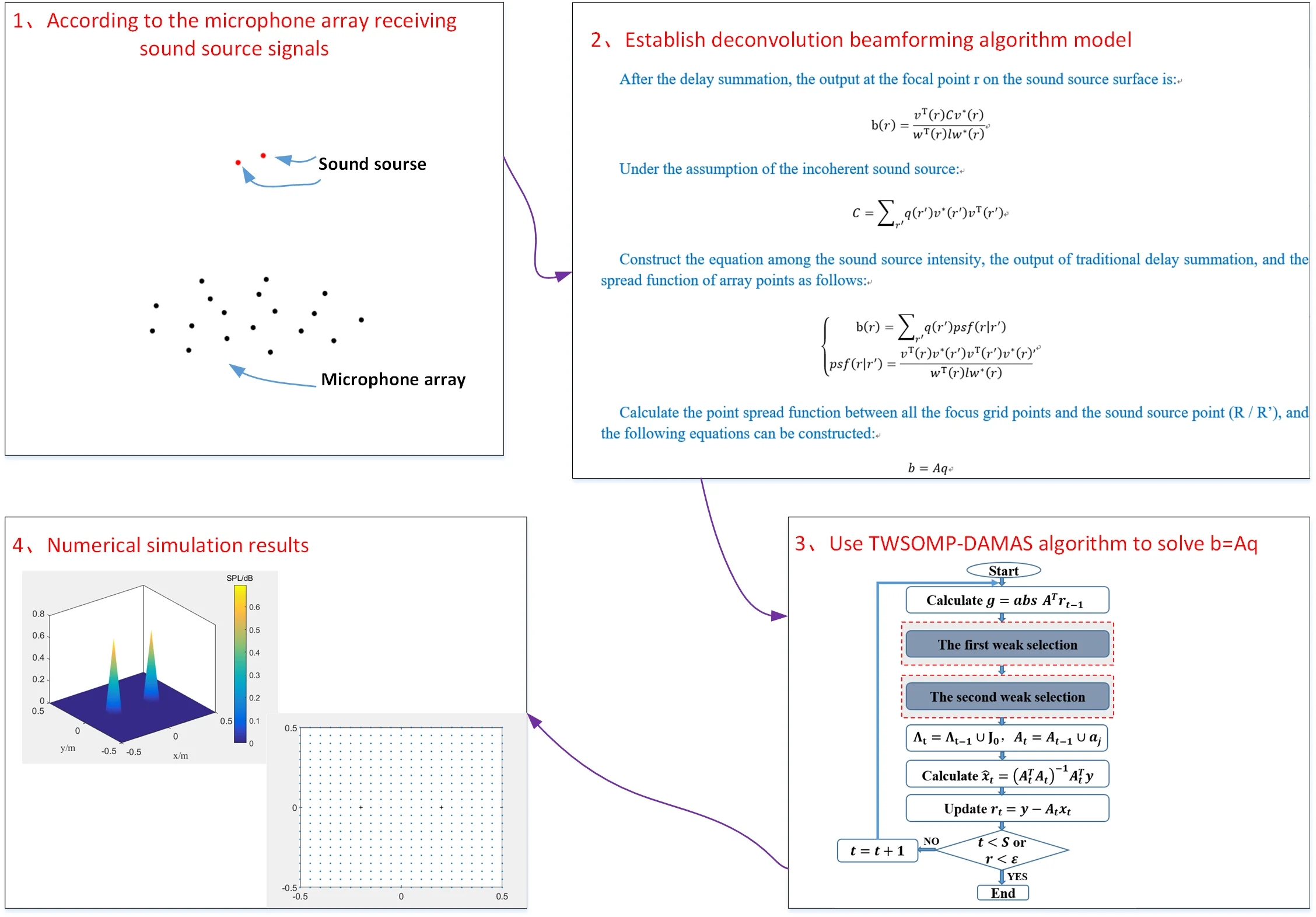
The traditional beamforming technology is based on the microphone array receiving the signal value of the sound source, discretizing the sound source plane into a certain number of focusing grid points, and performing reverse focusing on the focusing grid points through the delay summation algorithm, to enhance the output of the real sound source in the direction of the concentrate point and attenuate the production of other focusing points, and then effectively identify the sound source.

After the delay summation, the output at the focal point r on the sound source surface is:

1

b (r) = \frac{v^{T} (r) C v^{*} (r)}{w^{T} (r) l w^{*} (r)},

where $C$ is the cross spectrum matrix of sound pressure signals received by the microphone array; $l$ is a matrix in which all elements are 1; $v (r) = {[v_{1} (r), v_{2} (r), \dots, v_{m} (r)]}^{T}$ is the steering vector at the focal grid point $r$ ; $w (r) = {[{|v_{1} (r)|}^{2}, {|v_{2} (r)|}^{2}, \dots, {|v_{m} (r)|}^{2}]}^{T}$ ； $T$ and * represent transposition and conjugation, respectively; $v_{m} (r)$ represents the steering vector of the $m$ th microphone, it is expressed as:

2

v_{m} (r) = \frac{e^{- j k |r_{m} - r_{n}|}}{|r_{m} - r_{n}|} .

Under the assumption of the incoherent sound source, the sound pressure cross spectrum matrix $C$ can be expressed as:

3

C = \sum_{r^{'}} q (r^{'}) v^{*} (r^{'}) v^{T} (r^{'}),

where $r^{'}$ is the sound source position vector; $q (r^{'})$ is the sound source intensity at $r^{'}$ . Substituting Eq. (3) into Eq. (1) can construct the equation among the sound source intensity, the output of traditional delay summation, and the spread function of array points as follows:

4

\{\begin{array}{l} b (r) = \sum_{r^{'}} q (r^{'}) p s f (r| r^{'}), \\ p s f (r| r^{'}) = \frac{v^{T} (r) v^{*} (r^{'}) v^{T} (r^{'}) v^{*} (r)}{w^{T} (r) l w^{*} (r)}, \end{array}

where: $p s f (r| r^{'})$ is the array point propagation function, which is the contribution of the unit sound source intensity point sound source at $R^{'}$ position to the beamforming at the discrete focal point $R$ . Calculate the point spread functions of all the focus grid points and the sound source points $(r| r^{'})$ , then it can form an $N$ × $N$ dimensional point spread function $A$ . Thus, the following linear equations can be constructed:

5

b = A q,

where: $b = {(b_{1}, b_{2}, \dots b_{n})}^{H}$ is the column vector of $N$ -dimensional beamforming output, and $q = {({|q_{1}|}^{2}, {|q_{2}|}^{2}, \dots, {|q_{n}|}^{2})}^{H}$ is the $N$ -dimensional column vector composed of the sound source signal to be found on the sound source surface. The traditional deconvolution method adopts the Gaussian Saidel iteration method to solve it iteratively, and SC-DAMAS solves the equations by imposing L1 norm constraint on the strong power distribution of the sound source. OMP-DAMAS uses an orthogonal matching pursuit algorithm to solve it.

3. Twice weak selection orthogonal matching pursuit algorithm

3.1. Twice weak selection criterion

To solve the problem of over-reliance on the sparsity of sound source, this paper proposes an improved algorithm of orthogonal matching pursuit algorithm to solve the above linear equations; it can realize the accurate reconstruction of sound source position under the condition that the sparsity of sound source is unknown. Through the first weak selection criteria, the initial atom set is screened, and the wrong atoms are deleted. Under normal circumstances, there are still many wrong atoms after the first weak selection. Therefore, it is necessary to test the reliability of the previously selected atoms, then make the second weak selection to delete the chosen previously wrong atoms from the current atom set, and gradually delete all the false atoms in the form of iteration to get the final result. The following are the criteria for two weak elections.

The first weak selection criterion: the index of the inner product of the searched column is expanded from the original single maximum value to the number satisfying the condition of threshold coefficient α multiplied by the maximum internal product value.

Second weak selection criterion: arrange the values in the least square solution ( ${\hat{θ}}_{t}$ ) in descending order, and then select all the values before the maximum change rate. The calculation formula of the maximum change rate is:

6

H_{e} = \frac{|θ_{e} - θ_{e - 1}|}{θ_{e}},

where $θ_{e}$ is the $e$ value of the least square solution ${\hat{θ}}_{t}$ in ascending order.

3.2. TWSOMP-DAMAS algorithm specific steps

Given the $N$ × $N$ dimensional point spread function matrix $A$ , the column vector b of the $N$ dimensional beamforming output, the number of iterations $S =$ 10, and the threshold coefficient $α =$ 0.8.

Step 1: The initial conditions are: residual $γ_{0} = b$ , atomic support set $Λ_{0} = \emptyset$ , support matrix $A_{0} = 0$ , iteration number $t =$ 1.

Step 2: Find the index set $λ_{t}$ : $F_{f} = \max_{j = 1,2, 3, \dots, N} |〈γ_{t - 1}, {a_{j}}^{H}〉|$ , where $a_{j}$ is the $j$ th column of $A$ , $λ_{t} = \{j| F_{j} \geq α ∙ F_{f}\}$ .

Step 3: Update atom support set: $Λ_{t} = Λ_{t - 1} \cup λ_{t}$ , update support matrix $A_{t} = A_{t - 1} \cup a_{λ}$ , if $Λ_{t} = Λ_{t - 1}$ (that is, no new atoms are selected), stop iteration and go to step 9.

Step 4: Find the least square solution of $b = A_{t} θ_{t}$ : ${\hat{θ}}_{t} = a r g \min_{θ_{t}} {‖b - A_{t} θ_{t}‖}_{2} = {({A_{t}}^{T} A_{t})}^{T} {A_{t}}^{T} b$ .

Step 5: After ranking the values in the least square solution $θ_{t}$ from the largest to the smallest, calculate the change rate between two adjacent values, delete the values with the largest change rate in $θ_{t}$ , delete the column numbers corresponding to these values from the atomic support set $Λ_{t}$ , and update the atomic support set $Λ_{t}$ and the support matrix $A_{t}$ again.

Step 6: The least square solution of $b = A_{t} θ_{t}$ after calculating the updated atomic support set: ${\hat{θ}}_{t} = a r g \min_{θ_{t}} {‖b - A_{t} θ_{t}‖}_{2} = {({A_{t}}^{T} A_{t})}^{T} {A_{t}}^{T} b$ .

Step 7: Update residual: $γ_{t} = b - A_{t} {\hat{θ}}_{t} = y - {(A_{t}^{T} A_{t})}^{- 1} A_{t}^{T} b$ .

Step 8: $t = t + 1$ , if $t < S$ , go back to step 2 to continue iteration, if $t > S$ or residual $r_{t}$ reaches accuracy, stop iteration and enter step 9.

Step 9: The reconstructed $θ_{t}$ has a non-zero term at $λ_{t}$ , the values are $θ_{t}$ obtained in the last iteration, and the rest positions are 0.

4. Numerical simulation

In order to verify the feasibility and advantages of the proposed method, the recognition imaging results of the plane where the sound source is located are simulated and compared with SC-DAMAS algorithm and OMP-DAMAS algorithm for single sound source and double sound source. The influence of signal-to-noise ratio (SNR) on the algorithm identification in this paper is explored, and the accuracy of the algorithm in sound source identification is analyzed. It is assumed that the point sound source in space is located on the focal plane, its coordinates are (0, 0, 0.8), 20 dB white Gaussian noise is added, and an 18-channel microphone array is adopted. The size of the sound source plane is 1 m×1 m, which is evenly divided into 21×21 focal grid points, and the distance between the microphone array and the sound source plane is 0.8 m.

After many simulations, the TWSOMP-DAMAS algorithm can get a good reconstruction effect when the threshold coefficient parameter $α$ is 0.8, and the iteration number is 10 times.

4.1. Influence on frequency identification results

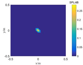
SC-DAMAS algorithm, OMP-DAMAS algorithm, and TWSOMP-DAMAS algorithm are used to locate the sound source at a single sound source frequency of 2500 Hz and a double sound source frequency of 5000 Hz, respectively, and the signal-to-noise ratio is 20 dB. The results are shown in Figs. 1 and 2.

Fig. 1The location results of 2500 Hz sound source

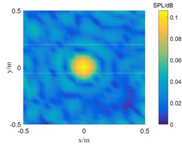
a) SC-DAMAS

b) OMP-DAMAS

c) TWSOMP-DAMAS

Fig. 1 shows the result of single sound source identification at 2500 Hz. SC-DAMAS algorithm, OMP-DAMAS algorithm, and TWSOMP-DAMAS algorithm can accurately identify the sound source position, but the identification result of SC-DAMAS algorithm has a large main lobe. TWSOMP-DAMAS algorithm can effectively reduce the width of the main lobe under the condition of unknown sound source sparsity, ensuring the same high identification accuracy and spatial resolution as OMP-DAMAS algorithm. Fig. 2 shows the identification results of 5000 Hz double sound sources. SC-DAMAS algorithm can't accurately identify the main sound source, and there are many pseudo-sound sources in the non-sound source position. On the contrary, OMP-DAMAS algorithm and TWSOMP-DAMAS algorithm can accurately locate the two sound sources, and TWSOMP-DAMAS algorithm can still achieve high-precision identification when the number of sound sources is unknown, which shows the advantages of TWSOMP-DAMAS algorithm.

Fig. 2The location results of 5000 Hz sound source

a) SC-DAMAS

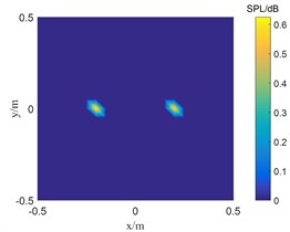
b) OMP-DAMAS

c) TWSOMP-DAMAS

4.2. Robustness verification of the algorithm

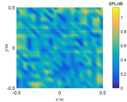
To further verify the influence of signal-to-noise ratio on TWSOMP-DAMAS algorithm, the frequency is 3500 Hz, and the distance between the microphone array and the focal plane of the sound source is 0.8 m m. The recognition results of single sound source under the conditions of 15 dB, 5 dB, and 0 dB are studied.

Fig. 3Results of single sound source localization

a) 0 dB

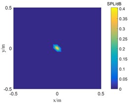
b) 5 dB

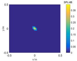
c) 15 dB

Fig. 3 shows the sound source identification results with signal-to-noise ratios of 0 dB, 5 dB and 15 dB, respectively. When the signal-to-noise ratio is 5 dB and 15 dB, the TWSOMPDAMAS algorithm can accurately locate the sound source. However, as the signal-to-noise ratio decreases to 0 dB, the position of the sound source identified by TWSOMP-DAMAS algorithm shifts downward by one grid compared with the position of the real sound source, which indicates that TWSOMP-DAMAS algorithm will be affected by excessive noise.

4.3. Accuracy analysis of recognition results

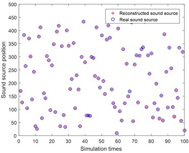
In order to verify the accuracy and stability of TWSOMP-DAMAS algorithm in identifying the sound source position, the frequency of a single sound source is 4500 Hz, the measuring surface is an 18-channel microphone array, the distance from the microphone array to the focus surface of the sound source is 0.8 m, and the signal-to-noise ratio is 20 dB. The results are shown in the Fig. 4.

Fig. 4 shows the recognition results of randomly assigning sound sources to any position on the sound source surface. It can be seen that TWSOMP-DAMAS algorithm has extremely high recognition stability, and it can accurately recognize the sound source positions in the process of recognizing 100 sound sources at any position.

Fig. 4Results of single sound source localization

5. Conclusions

TSWOMP-DAMAS algorithm solves the precondition of over-reliance on the sparsity of sound source, so it has greater advantages in practical engineering application. The simulation results show that when the frequency is the same, TWSOMP-DAMAS algorithm can accurately locate single and double sound sources under the premise that the sparsity of sound sources is unknown. Compared with SC-DAMAS algorithm, TWSOMP-DAMAS algorithm can effectively reduce sidelobe, improve spatial resolution and ensure the same reconstruction accuracy as OMP-DAMAS algorithm. The TWSOMP-DAMAS algorithm proposed in this paper has high recognition accuracy and good adaptability to noise when the frequency is 3500 Hz and the signal-to-noise ratio is greater than 0 dB. In 100 times of sound source identification at random positions, this algorithm can accurately identify the sound source position, which proves that the TWSOMP-DAMAS algorithm has good stability and high accuracy.

References

T. F. Brooks and W. M. Humphreys, “A deconvolution approach for the mapping of acoustic sources (DAMAS) determined from phased microphone arrays,” Journal of Sound and Vibration, Vol. 294, No. 4-5, pp. 856–879, Jul. 2006, https://doi.org/10.1016/j.jsv.2005.12.046

Publisher
Y. Yang and Z. G. Chu, “A review of high-performance beamforming methods for acoustic source identification,” (in Chinese), Journal of Mechanical Engineering, Vol. 57, No. 24, pp. 166–1183, 2021.

Publisher
Y. Yang, J. M. Ni, and Z. G. Chu, “Engine noise source identification based on DAMAS2 beamforming,” (in Chinese), Chinese Internal Combustion Engine Engineering, Vol. 35, No. 2, pp. 59–65, 2014.

Search CrossRef
Y. Yang, J. Zhang, and B. He, “Analysis on exterior noise characteristics of high-speed trains in bridges and embankments section based on experiment,” (in Chinese), Journal of Mechanical Engineering, Vol. 55, No. 20, pp. 188–197, 2019.

Search CrossRef
K. Ehrenfried and L. Koop, “Comparison of iterative deconvolution algorithms for the mapping of acoustic sources,” AIAA Journal, Vol. 45, No. 7, pp. 1584–1595, Jul. 2007, https://doi.org/10.2514/1.26320

Publisher
O. Lylloff, E. Fernández-Grande, F. Agerkvist, J. Hald, E. Tiana Roig, and M. S. Andersen, “Improving the efficiency of deconvolution algorithms for sound source localization,” The Journal of the Acoustical Society of America, Vol. 138, No. 1, pp. 172–180, Jul. 2015, https://doi.org/10.1121/1.4922516

Publisher
R. P. Dougherty, R. C. Ramachandran, and G. Raman, “Deconvolution of sources in aeroacoustic images from phased microphone arrays using linear programming,” in 19th AIAA/CEAS Aeroacoustics Conference, Vol. 12, No. 7, pp. 699–718, May 2013, https://doi.org/10.2514/6.2013-2210

Publisher
R. Dougherty, “Extensions of DAMAS and benefits and limitations of deconvolution in beamforming,” in 11th AIAA/CEAS Aeroacoustics Conference, pp. 2961–2974, May 2005, https://doi.org/10.2514/6.2005-2961

Publisher
L. Shen, Z. Chu, Y. Yang, and G. Wang, “Periodic boundary based FFT-FISTA for sound source identification,” Applied Acoustics, Vol. 130, pp. 87–91, Jan. 2018, https://doi.org/10.1016/j.apacoust.2017.09.009

Publisher
J. Shi, D. S. Yang, and S. G. Shi, “Compressive focused beamforming based on vector sensor array,” Acta Physica Sinica, Vol. 65, No. 2, pp. 194–204, 2016.

Publisher
F. Ning, “Study on sound sources localization using compressive sensing,” Journal of Mechanical Engineering, Vol. 52, No. 19, pp. 42–52, 2016, https://doi.org/10.3901/jme.2016.19.042

Publisher
T. Yardibi, J. Li, P. Stoica, and L. N. Cattafesta, “Sparsity constrained deconvolution approaches for acoustic source mapping,” The Journal of the Acoustical Society of America, Vol. 123, No. 5, pp. 2631–2642, May 2008, https://doi.org/10.1121/1.2896754

Publisher
T. Padois and A. Berry, “Orthogonal matching pursuit applied to the deconvolution approach for the mapping of acoustic sources inverse problem,” The Journal of the Acoustical Society of America, Vol. 138, No. 6, pp. 3678–3685, Dec. 2015, https://doi.org/10.1121/1.4937609

Publisher

About this article

Received

09 May 2022

Accepted

29 May 2022

Published

13 June 2022

SUBJECTS

Acoustics, noise control and engineering applications

DOI

https://doi.org/10.21595/vp.2022.22718

Keywords

deconvolution

number of sound sources

sound sources localization

TWSOMP-DAMAS

Acknowledgements

This work was supported by the Natural Science Basic Research Program of Shaanxi (Program No. 2022JM271) and the Postdoctoral research project of Shaanxi Province (Grant No. 2018BSHEDZZ10).

This is an open access article distributed under the Creative Commons Attribution License, which permits unrestricted use, distribution, and reproduction in any medium, provided the original work is properly cited.

Previous article in issue Previous Next article in issue Next

Research article

2023 02 09

An improved deconvolution beamforming algorithm for acoustic imaging of low signal-to-noise ratio sound sources in reverberant field

Wenyong Guo, Hantao Chen, Jing Xia, Xiaofeng Li, Chenghao Cao

Research article

2022 08 15

A review for the noise source identification methods based microphone array

Junjian Hou, Li Zeng, Dengfeng Zhao, Yudong Zhong

Research article

2022 05 15

An adaptive beamforming algorithm for sound source localisation via hybrid compressive sensing reconstruction

Wenyong Guo, Jianggui Han, Hantao Chen, Li Yu, Zhe Wu

Research article

2021 06 28

A method of sound source recognition based on tow weak selection compressed sensing

Yuxi Chen, Jin Mao, Yahui Cui

W. Zhao, J. Mao, and K. Liu, “A deconvolution sound source identification method based on twice weak selection orthogonal matching pursuit,” Vibroengineering PROCEDIA, Vol. 43, pp. 102–108, Jun. 2022, https://doi.org/10.21595/vp.2022.22718

Copy Extrica

Copied to clipboard!

TY  - JOUR
DO  - 10.21595/vp.2022.22718
UR  - https://doi.org/10.21595/vp.2022.22718
TI  - A deconvolution sound source identification method based on twice weak selection orthogonal matching pursuit
T2  - Vibroengineering PROCEDIA
AU  - Zhao, Weipeng
AU  - Mao, Jin
AU  - Liu, Kai
PY  - 2022
DA  - 2022/06/13
PB  - JVE International Ltd.
SP  - 102-108
VL  - 43
SN  - 2345-0533
SN  - 2538-8479
ER  - 

Copy Ris

Copied to clipboard!

@article{Zhao_2022,
	doi = {10.21595/vp.2022.22718},
	url = {https://doi.org/10.21595/vp.2022.22718},
	year = 2022,
	month = {jun},
	publisher = {{JVE} International Ltd.},
	volume = {43},
	pages = {102--108},
	author = {Weipeng Zhao and Jin Mao and Kai Liu},
	title = {A deconvolution sound source identification method based on twice weak selection orthogonal matching pursuit},
	journal = {Vibroengineering {PROCEDIA}}
}

Copy Bibtex

Copied to clipboard!

[1]W. Zhao, J. Mao, and K. Liu, “A deconvolution sound source identification method based on twice weak selection orthogonal matching pursuit,” Vibroengineering PROCEDIA, vol. 43, pp. 102–108, Jun. 2022, doi: 10.21595/vp.2022.22718.

Copy IEEE

Copied to clipboard!

Zhao, Weipeng, Jin Mao, and Kai Liu. “A Deconvolution Sound Source Identification Method Based on Twice Weak Selection Orthogonal Matching Pursuit.” Vibroengineering PROCEDIA 43 (June 13, 2022): 102–8. https://doi.org/10.21595/vp.2022.22718.

Copy Chicago

Copied to clipboard!

A deconvolution sound source identification method based on twice weak selection orthogonal matching pursuit

Abstract

Highlights

1. Introduction

2. Theoretical basis of deconvolution beamforming

3. Twice weak selection orthogonal matching pursuit algorithm

3.1. Twice weak selection criterion

3.2. TWSOMP-DAMAS algorithm specific steps

4. Numerical simulation

4.1. Influence on frequency identification results

4.2. Robustness verification of the algorithm

4.3. Accuracy analysis of recognition results

5. Conclusions

References

About this article

Related Articles