An improved deconvolution beamforming algorithm for acoustic imaging of low signal-to-noise ratio sound sources in reverberant field

Guo, Wenyong; Chen, Hantao; Xia, Jing; Li, Xiaofeng; Cao, Chenghao

doi:10.21595/jve.2022.22634

Journal of Vibroengineering

Browse Journal

Submit article

Published: 09 February 2023

Check for updates

An improved deconvolution beamforming algorithm for acoustic imaging of low signal-to-noise ratio sound sources in reverberant field

Wenyong Guo¹

Hantao Chen²

Jing Xia³

Xiaofeng Li⁴

Chenghao Cao⁵

^{1, 2, 4, 5}College of Power Engineering, Naval University of Engineering, Wuhan, China

³Military Representative Bureau of the Naval Armament Department in Guangzhou, Guangzhou, China

Corresponding Author:

Xiaofeng Li

Cite the article Download PDF

Downloads 235

Abstract

Most of the existing acoustic imaging studies in reverberant field ignore the influence of signal-to-noise ratio. As a result, commonly used beamforming algorithms in reverberant backgrounds have poor imaging accuracy for low signal-to-noise ratio sound sources. In response to that problem, an improved adaptive beamforming algorithm called SC-DAMAS is put forward in this paper. The algorithm replaces the free-field Green's function with the impulse response function, making the algorithm more suitable for acoustic imaging of low signal-to-noise ratio in a reverberant environment. Besides, the comparative simulation results with the conventional beamforming method and orthogonal matching pursuit algorithm-based DAMAS, as well as sound source acoustic imaging experiments are carried out to analyze its effectiveness. It is indicated that, in the reverberation field, the SC-DAMAS has no obvious sidelobes and achieves higher positioning accuracy for acoustic imaging of low signal-to-noise ratio sound source than the abovementioned counterparts, and its imaging test result is consistent with the actual situation, which verifies the effectiveness of the algorithm.

An improved deconvolution beamforming algorithm for acoustic imaging of low signal-to-noise ratio sound sources in reverberant field

Highlights

By introducing the free-field Green's function, an improved adaptive beamforming algorithm, called SC-DAMAS, is put forward in this paper for acoustic imaging of low signal-to-noise ratio in a reverberant environment.
Comparative simulations among the SC-DAMAS and other classical algorithms in different signal-to-noise ratio scenarios indicate the proposed algorithm has no obvious sidelobes and achieves higher positioning accuracy.
Sound source acoustic imaging experiments of SC-DAMAS in a real ship engine cabin further show that its imaging result is consistent with the actual situation, which verifies the effectiveness of the algorithm.

1. Introduction

A reverberant sound field is formed when sound waves propagate in a closed indoor environment, as they will continuously be reflected and absorbed while encountering walls or other obstacles. In reverberant field, in addition to the direct sound wave from the sound source, the reflected sound after reflections of the original sound wave and external noise is also collected by the sensor array. Therefore, sound source localisation in a reverberant environment is far more complicated than that in the free field, which brings a challenge to the sound source localisation work [1].

In general, signal processing and acoustic imaging are two main parts of sound sources localisation in a reverberation field. For the signal processing part, compressive sensing (CS) is a widely adopted technology. In the CS technique, signals are acquired by sub-Nyquist rates of traditional signal processing [2]. It gets rid of the limitation that the sampling frequency needs to be at least twice the highest frequency of the original signal to accurately recover the information in the signal [3]. For instance, based on sparse recovery in CS, a multi-channel deconvolution algorithm was proposed to enhance the source signal by Ping et al. [4]. Besides, on the basis of sparse representation, Wang et al. [5] combined the variational Bayesian expectation-maximization method to solve the equation and studied the sound source localisation in the reverberant environment. Thanks to the previous valuable investigations, more CS reconstruction algorithms have been developed for acoustic beamforming, like Orthogonal Matching Pursuit [6], Regularized OMP [7], Compressive Sampling Matching Pursuit (CoSaMP) [8], Variable step-size Gradient Matching Pursuit [9], Stochastic Gradient Matching Pursuit [10] and sparsity adaptive matching pursuit (SAMP) [11]. Among them, the SAMP algorithm is adaptive to its sparsity value but has unstable reconstruction accuracy and sensitive running speed to the iteration step size. More specifically, too small a step size can lead to insufficient sparsity estimation, which increases the number of algorithm iterations and thereby reduces the algorithm efficiency. On the other hand, sparse overestimation problem is generated with too large a step size, and further negatively affects the reconstruction accuracy of the signal. As for the CoSaMP algorithm, it owns a speed advantage with predetermined sparsity. Therefore, it is inspired that hybrid algorithm combining SAMP and CoSaMP can maintain the speed advantage and adaptive searching ability for sparsity.

As for specific acoustic imaging in a reverberation field, it generally involves the beamforming solution and interference suppression. For instance, combined with the array signal processing technology, Peled et al. [12] studied the reverberation suppression algorithm in the circular sensor array, which decreases the negative effects of the reflected sound waves. Aiming at acoustic imaging after long reverberation time, a general cross-correlation classification algorithm was proposed by Sun et al. [13] to improve robustness to reverberation environmental changes. Meanwhile, based on the principle of matrix low-rank characteristics, Xu et al. [14] reported an improved method, and based on dithering technology, Hao et al. [15] proposed a GCC-IWF algorithm for underwater reverberation environment. All of them contributed to improving the accuracy of acoustic imaging in a reverberant field. For the interference suppression, Nahma et al. [16] proposed a robust beamforming algorithm based on the room impulse response, which improved the algorithm's robustness in different reverberant environments. Rajan et al. [17] used the wavelet denoising method for time delay estimation, which effectively reduced the influence of underwater reverberation on sound source localisation. Jiang et al. [18] proposed a new algorithm combining deep fusion and Convolutional Neural Network in response to the problem of inaccurate sound source localisation in a reverberant environment. Combining double-wide matching pursuit method, Fang et al. [19] proposed a multi-sound source localisation counting technique. The sound source location accuracy and absolute error analysis results show that this methodology has better accuracy in the conditions of strong reverberation and multiple sound sources. Kilis et al. [20] proposed a new speech de-reverberation algorithm and carried out experimental verification in the actual reverberation environment. Fischer et al. [21] modified the cross-correlation matrix of the array sound pressure signal to effectively improve the beamforming accuracy in the reverberant environment. Based on the statistical characteristics of binaural signals and the difference in amplitude spectrum, Ghamdan et al. [22] proposed a new algorithm. This algorithm can be applied to different reverberation rooms and weaken the dependence on relevant environmental parameters.

In the real environment, the actual ship cabin generally belongs to a narrow and closed space with unavoidable indoor reverberation, which further aggravates the difficulty of locating the target sound source. Therefore, it is very necessary to carry out acoustic imaging research in reverberation field under low signal-to-noise ratio condition. For that purpose, we analyzed the propagation law of sound waves in the reverberation field, and construct the room impulse response function to reconstruct the connection between the sound source and the array. Replacing the free-field Green's function with the newly constructed room impulse response function results in an improved beamforming algorithm for acoustic imaging in reverberant field. To demonstrate its accuracy, we perform comparative simulation analysis with the conventional beamforming method (CBF), as well as orthogonal matching pursuit algorithm-based deconvolution approach (OMP-DAMAS) in different frequencies. It is indicated that among the three techniques, SC-DAMAS owns the best positioning accuracy of sound in reverberant field.

The rest of the article is organised as follows. Section 2 describes the theoretical background and our adaptive beamforming algorithms. Section 3 introduces the simulation model and contrastive analysis of sound source localisation. Section 4 presents the experimental results that prove the superiority of our adaptive beamforming algorithms. Lastly, Section 5 discusses this study’s conclusions.

2. Material and methods

2.1. Sound radiation model of reverberation field

In the actual working cabin or room, the sound waves radiated by the sound source will encounter obstacles such as walls, ceilings, tables, and chairs when propagating. These obstacles will reflect and absorb the sound waves to a certain extent. As the number of collisions increases, the amount of sonic energy attenuated also increases. In this case, the sound wave is reflected back and forth in all directions and gradually attenuated, which forms the reverberation field. Therefore, the signals received by the sensor array are not all direct sound waves from the sound source, but also contain a large number of reflected sound waves.

Similar to the free-field Green's function, there is also a transfer function in the reverberation field to connect the sound source signal and the sensor array receiving signal. This transfer function is called the room impulse response function. In the indoor reverberation environment, the acoustic signal received by the array is:

1

y (t) = \int_{0}^{+ \infty} h (τ) x (t - τ) d τ + n (t) = h (t) * x (t) + n (t),

where $y (t)$ is the signal received by the sensor array, $h (t)$ is the indoor impulse response function, $x (t)$ is the sound source signal, $n (t)$ is the noise signal, $τ$ is the delay caused by the sound wave reflection, and $*$ is the convolution operation. Then perform Fourier transform to the frequency domain, it can be described as follows:

2

Y (ω) = X (ω) H (ω) + N (ω),

where $Y (w)$ , $X (w)$ , $H (w)$ , and $N (w)$ in Eq. (2) are obtained by Fourier transform of $y (t)$ , $x (t)$ , $h (t)$ , and $n (t)$ in Eq. (1), respectively. It can be seen that the indoor impulse response function plays a role in the connection between the sound source and the signal received by the sensor array, so accurate acquisition of the indoor impulse response function is very important for the reproduction of the sound field.

2.2. Indoor impulse response calculation

The mirror source method employs related acoustic software to simulate and obtain the impulse response function. It has good convenience and practicability and is a widely used computer simulation method. The core idea of this technique is to treat the reflected sound wave as a direct sound wave from the mirror sound source to the sensor, and then use the position relationship between the mirror sound source and the sensor to calculate the sound path. At the same time, considering the reflection coefficient of each wall, calculate the energy attenuation of the sound wave in the reflection process, thereby constructing the indoor impulse response function:

3

h (t) = \sum_{p = 1}^{8} \sum_{r = - \infty}^{\infty} β_{x, 1}^{|n_{x} - q|} β_{x, 2}^{|n_{x}|} β_{y, 1}^{|n_{y} - j|} β_{y, 2}^{|n_{y}|} β_{z, 1}^{|n_{z} - k|} β_{z, 2}^{|n_{z}|} \frac{δ [t - \frac{|R_{p} + R_{r}|}{c}]}{4 π |R_{p} + R_{r}|} .

Further convert Eq. (3) to frequency domain:

4

H (ω) = \sum_{p = 1}^{8} \sum_{r = - \infty}^{\infty} β_{x, 1}^{|n_{x} - q|} β_{x, 2}^{|n_{x}|} β_{y, 1}^{|n_{y} - j|} β_{y, 2}^{|n_{y}|} β_{z, 1}^{|n_{z} - k|} β_{z, 2}^{|n_{z}|} \frac{e^{i \frac{ω}{c} |R_{p} + R_{r}|}}{4 π |R_{p} + R_{r}|} e^{- i ω t} .

Assuming that the actual sound source point coordinates are $(x, y, z)$ , the sensor array element coordinates are $(x', y', z')$ , and the room size are $(L_{x}, L_{y}, L_{z})$ , then:

5

R_{p} = (x - x' + 2 q x', y - y' + 2 j y', z - z' + 2 k z'),

6

R_{r} = 2 (n_{x} L_{x}, n_{y} L_{y}, n_{z} L_{z}),

where $R_{p}$ represents the distance from the actual sound source or mirror image source to each array element. $R_{r}$ represents the virtual space size corresponding to the multi-order reflection. $c$ is the speed of sound. $β_{x, 1}$ , $β_{y, 1}$ , and $β_{z, 1}$ represent the reflection coefficient of the wall close to the origin of the coordinate in three directions, respectively. $β_{x, 2}$ , $β_{y, 2}$ , and $β_{z, 2}$ represent the reflection coefficients of walls far from the origin of the coordinates in three directions, respectively. The acoustic characteristics of each wall are often expressed by the sound absorption coefficient, and the reflection coefficient is calculated by $β = \pm \sqrt{1 - γ}$ , in which $γ$ is the sound absorption coefficient of the wall. $(n_{x}, n_{y}, n_{z})$ is the value range of each element, which forms an integer set related to the reflection order. It is worth mentioning that, as parameters $q$ , $j$ , $k$ can be 0 or 1, there exists 8 possible analytical solutions.

2.3. Adaptive beamforming method

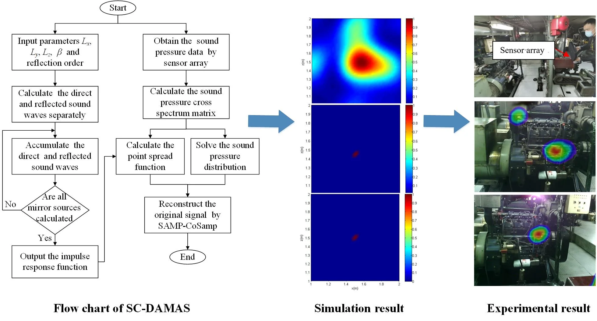
In general, the sensor array receiving signal and the sound source signal is connected by a transfer function, and different sound field environments correspond to different transfer functions. In the free field, the transfer function is the free field Green’s function, while in the reverberation scenarios, the transfer function becomes the room impulse response function. Therefore, for sound source localisation in the background of reverberation, the free-field Green’s function is firstly replaced with the indoor impulse response function. Then as shown in Fig. 1, combining the advantages of the classic CoSaMP and SAMP algorithms, an improved beamforming algorithm can be obtained.

Fig. 1Flow chart of the improved algorithm

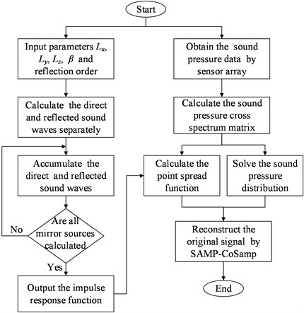
In the previous study, a hybrid compressive sensing reconstruction algorithm called SAMP-CoSamp was proposed. For sound source imaging, combines the speed advantage of CoSaMP algorithm and the adaptive sparsity searching ability from the SAMP algorithm. It enhances the acoustic imaging performance in free-field condition since a good balance between running efficiency and reconstruction error is stroke. Details about this part of modeling can be found in the authors’ previous research work [23]. Its naive beamforming mechanism can be described in Table 1.

Table 1Algorithm 1 for SAMP-CoSamp

1: Input the initial parameters

K

,

L

, and

F

as

K =

1,

L = s

, and

F = Ф

, respectively

2: Calculate the correlation coefficient by

u = \{u_{j} |u_{j} = |⟨r, ϕ_{j}⟩|, j = 1,2, \dots N\}

, extract the index value with respect to the

K

maximum values and store them in set

F

3: If

{‖Φ_{F}^{T} y‖}_{2} \leq \frac{1 - δ_{K}}{\sqrt{1 + δ_{K}}} {‖y‖}_{2}

4:

K = K_{0} + L

5: else

6: continue step 2

7: end

8: Calculate the initiate margin by

r = y - Φ_{F} Φ_{F}^{+} y

9: Set the initial parameters as

x =

0, stage = 1, and

k =

1

10: Calculate the correlation coefficient by

u = \{u_{j} |u_{j} = |⟨r, ϕ_{j}⟩|, j = 1,2, \dots N\}

and then store the corresponding index value in the index set if

u_{j} \geq 0.5 m a x |u|

11: Calculate the correlation coefficient by

u = \{u_{j} |u_{j} = |⟨r, ϕ_{j}⟩|, j = 1,2, \dots N\}

, Then extract the index values with respect to the k maximum values and store them in the new set

F_{n e w}

12: Calculate the estimated signal by

x_{n e w} = a r g m i n {‖y - Φ_{{\tilde{Λ}}_{t}} x‖}_{2}

and update the margin

r_{n e w} = y - Φ_{F} x

.

13: If

{‖x_{n e w} - x‖}_{2} \leq ε

14: stop the iteration

15: else

16: skip to step 18

17: end

18 : If

{‖r_{n e w}‖}_{2} \geq {‖r‖}_{2}

19: stage = stage + 1,

L =

stage*s

20: else

21:

F = F_{n e w}

,

r = r_{n e w} k = k + 1

, Afterwards, return to step 10

22: end

Parameters description:

y

→ measured sound pressure,

F

→ Final value set corresponding to the index,

x

→ Estimated sound source signal data,

k

→ Iterations number,

s

→ Step size,

u

→ Correlation coefficient,

⟨•, •⟩

→ Operator of vector’s inner product,

Φ_{j}

→

j

thcolumn measurement matrix

3. Simulation analysis

3.1. Simulation model building

Simulation is conducted to demonstrate the effectiveness of SC-DAMAS for sound source localisation issues. At first, a reverberation field area with a size of 3 m×4 m×3 m, is constructed in the COMSOL multiphysics simulation environment. Considering the different properties and characteristics of the reverberation field and the free field, we choose the ray acoustics module for modeling and simulation. A monopole source surrounded by air is set as the sound source at (1.5 m, 3 m, 1.5 m), and its power intensity is set to 10e-5 W. In order to better simulate the sound propagation process in the actual environment, the fluid model is set to atmospheric attenuation with the relative humidity of 50 % and the initial ray number of 10e5. When sound waves propagate to each wall surface, reflection and absorption will occur. The amount of reflection and absorption varies with the sound absorption coefficient of each wall surface. The measurement surface of sensor array is set at 1m from the sound source surface, whose array element spacing is 0.1 m, surface size is 1 m×1 m and array elements number is 11×11. The mesh division of the reverberation field and the schematic diagram of the sensor array position are shown in Fig. 2. Besides, it is worth mentioning that During the modeling process, we carefully consider the absorption coefficient of each wall. According to our investigation, the sound absorption coefficient of each wall at different frequencies is also shown in the Table 2.

Fig. 2Simulation model of the sound source in reverberant field

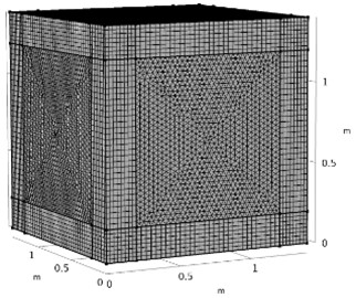
a) Mesh division

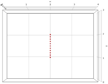
b) Schematic diagram of measurement array

Table 2Sound absorption coefficient of each wall of the room

Frequency (Hz)	125	250	500	1000	2000	4000
Front and left side	0.18	0.06	0.04	0.03	0.02	0.02
Right side and ceiling	0.1	0.05	0.06	0.07	0.09	0.08
Ground	0.01	0.01	0.01	0.01	0.02	0.02
Back side	0.35	0.25	0.18	0.12	0.07	0.04

To further study the applicability of the algorithm in the complex sound field background, the low signal-to-noise ratio factor is added to the reverberation background. More specifically, gaussian white noise with a relative amplitude of 0.01 times, 0.1 times, and 0.3 times is added to the obtained sound pressure data from measurement surface to simulate the noisy environment of SNR = 10 dB, respectively. Taking the collected sound pressure data under the frequency of 2000 Hz and the time of 0.1 s as an instance, Fig. 3 shows the sound pressure distribution in the measurement surface while Gaussian white noise with different relative amplitudes is added.

Fig. 3Sound pressure distribution of different SNR conditions

a) Noise-free

b) SNR = 10 dB

It can be seen from Fig. 3, under no-noise conditions, the sound pressure distribution on the measuring surface is relatively concentrated, and the approximate position of the sound source can be judged. After adding noise, the sound pressure distribution on the measuring surface gradually becomes fuzzy or even chaotic with increasing noise, and it is no longer possible to judge the position of the sound source through the sound pressure level distribution on the measuring surface. In the following text, the SC-DAMAS are applied for sound source localisation with the effects of white noise.

3.2. Acoustic imaging result

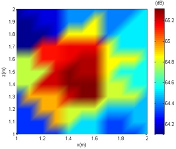
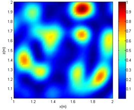
In a practice environment, the target sound source signal could be submerged by noise, especially for low SNR cases, which negatively affects the information extraction and imaging of the target sound source. Therefore, the sound source localisation issues under low SNR conditions is an urgent problem in engineering practice. In the study, the CBF [24], OMP-DAMAS [6], and SC-DAMAS are used to process the measured sound field data with SNR = 10 dB under different frequencies. The comparative pressure distributions of different frequency sounds are described in Fig. 4-6.

Fig. 4Comparative imaging results under the frequency of 1000 Hz

a) CBF

b) OMP-DAMAS

c) SC-DAMAS

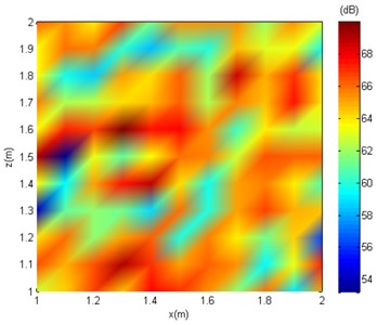
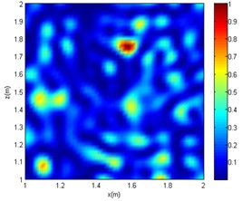
Fig. 5Comparative imaging results under the frequency of 2000 Hz

a) CBF

b) OMP-DAMAS

c) SC-DAMAS

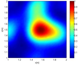
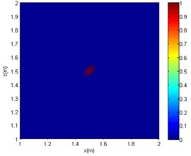
Fig. 6Comparative imaging results under the frequency of 4000 Hz

a) CBF

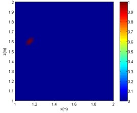
b) OMP-DAMAS

c) SC-DAMAS

It can be seen from Figs. 4-6 that in the reverberation field, for CBF, only an approximate range can be obtained at low frequencies. At medium and high frequencies, the acoustic imaging is chaotic, and there is obvious interference with greater intensity, which makes the localisation fail. As for the OMP-DAMAS method, in the reverberation field, the algorithm can maintain a certain degree of accuracy except for the low-frequency conditions. Although the imaging results have no sidelobes in the mid- and high-frequency conditions, they are seriously inconsistent with the actual sound source position. Superior to the CBF and OMP-DAMAS, the SC-DAMAS method has good localisation accuracy in a wide frequency range without sidelobe interference. The specific sound source localisation results by three methods are shown in Table 3.

Table 3Sound source localisation and algorithm efficiency comparison

Algorithm	CBF	OMP-DAMAS	SC-DAMAS
1000 Hz	(1.55 m, 1.5 m)	(1.5 m, 1.45 m)	(1.5 m, 1.5 m)
2000 Hz	(1.7 m, 1.95 m)	(1.8 m, 1.75 m)	(1.5 m, 1.55 m)
4000 Hz	(1.6 m, 1.75 m)	(1.15 m, 1.6 m)	(1.5 m, 1.45 m)

In summary, under the conditions of the same signal-to-noise ratio and the same sound source frequency, the sound source localisation result of the CBF method is far from the actual sound source position, and a certain intensity of interference sound source would appear. Although there are no interfering sound sources in the imaging results of the OMP-DAMAS method, there is a poor localisation accuracy at mid and high frequencies cases ( $f =$ 2000 or 4000 Hz). As the frequency increases, although the OMP-DAMAS imaging results have no obvious sidelobes, there is also the problem of reduced accuracy. The change of frequency has little effect on the SC-DAMAS method, and its imaging results achieve high accuracy, featuring no sidelobe effects, good stability, and reliability.

4. Test verification

In order to verify the acoustic imaging effectiveness of the proposed SC-DAMAS for the sound source of low signal-to-noise ratio in reverberant field, acoustic imaging experiments are carried out. An actual ship engine cabin with a size of 17.3 m×8.6 m×2.2 m is selected as the experimental site. As shown in Fig. 7(a), the main noise sources in the cabin are diesel generators and diesel engine. It is worth mentioning that the cabin is confined, and there is other equipment thus environmental noise is unavoidable. Therefore, the cabin forms a reverberation field, and its sound source features low signal-to-noise ratio. During the start of the ship, the main noise sources in the engine room are near the piston cylinder, the intake pipe, and the exhaust pipe. As for the stop phase, the main noise source is near the piston cylinder. In our experiment, both of the ship’s start and stop stages are considered to conduct acoustic imaging experiments. As shown in Fig. 7(b) and (c), the surveyor uses a handheld acoustic imaging test system to collect the sound source data 1.5 meters away.

After the experiment, the measured real-time sound pressure data by the sensor array are exported to the host computer and taken as the input of SC-DAMAS, and the obtained imaging results are shown in Fig. 8. It can be seen that the calculated noise position of the diesel generator during the ship’s start and stop stage is not the same. The main noise source during the start phase appears near the diesel engine piston cylinder, intake pipe, exhaust pipe, etc. As for the case of the stop stage, the main noise comes from the piston cylinder. Similar with the measurement results of diesel generator, the acoustic imaging of diesel engine by SC-DAMAS can locate the noise sources in the two stages. In the start up stage, the main noise source is located around the piston cylinder, intake and exhaust pipe. As for that of stop stage, the main noise is generated by piston cylinder. The Sound source localisation experiment of diesel generator and diesel engine in reverberant field is highly consistent with the actual situation. It is worth mentioning that there is more complex on-site interference than simulation environment, and the positioning accuracy needs to be improved. However, it can be seen in Fig.8 that a sufficiently precise position of noise source has been obtained, which is meaningful since it can give good guidance to engineers and technicians. In summary, the applicability of the reported algorithm for sound source localisation in reverberation is verified.

Fig. 7Sound source localisation experiment in reverberant field

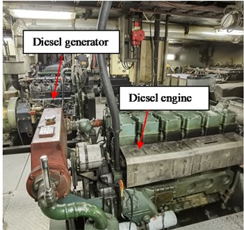
a) Ship engine cabin

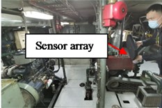
b) Diesel generator noise measurement

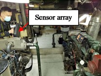
c) Diesel engine noise measurement

Fig. 8Experimental result of sound source imaging

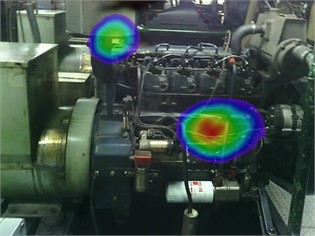
a) Star up of diesel generator

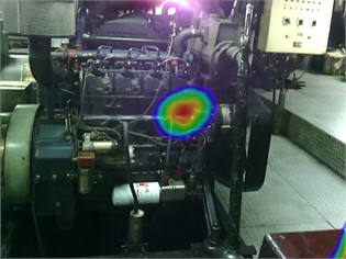
b) Stop of diesel generator

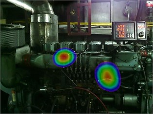
c) Star up of diesel engine

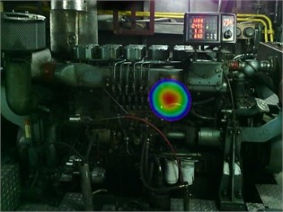
d) Stop of diesel engine

5. Conclusions

In this paper, an adaptive beamforming algorithm based on impulse response function is proposed in this paper, which can effectively reduce the interference caused by reverberation and low signal-to-noise ratio factors on acoustic imaging. For its adaptive feature, a hybrid compressive sensing reconstruction algorithm called SAMP-CoSaMP is proposed first. This hybrid algorithm not only gets rid of the dependence of the original CoSaMP on the sparsity but also alleviated the problem of inefficiency of the SAMP. Then combined with the DAMAS, the adaptive sound source localisation approach called SC-DAMAS is further put forward. Compared with the CBF and OMP-DAMAS, this method has better imaging accuracy under the background of low signal-to-noise ratio and reverberation, besides it is suitable for a wider frequency range. In the end, taking common marine machinery and equipment as the research object, an acoustic imaging experiment under the background of the relevant reverberation sound field is designed and carried out, which verifies the effectiveness of the algorithm in this paper.

References

M. Jia, Y. Jia, S. Gao, J. Wang, and S. Wang, “Multi-source DOA estimation in reverberant environments using potential single-source points enhancement,” Applied Acoustics, Vol. 174, p. 107782, Mar. 2021, https://doi.org/10.1016/j.apacoust.2020.107782

Publisher
D. L. Donoho, “Compressed sensing,” IEEE Transactions on Information Theory, Vol. 52, No. 4, pp. 1289–1306, Apr. 2006, https://doi.org/10.1109/tit.2006.871582

Publisher
E. Sejdić, I. Orović, and S. Stanković, “Compressive sensing meets time-frequency: An overview of recent advances in time-frequency processing of sparse signals,” Digital Signal Processing, Vol. 77, pp. 22–35, Jun. 2018, https://doi.org/10.1016/j.dsp.2017.07.016

Publisher
P. K. T. Wu, N. Epain, and C. Jin, “A dereverberation algorithm for spherical microphone arrays using compressed sensing techniques,” in ICASSP 2012 – 2012 IEEE International Conference on Acoustics, Speech and Signal Processing, pp. 4053–4056, Mar. 2012, https://doi.org/10.1109/icassp.2012.6288808

Publisher
L. Wang, Y. Liu, L. Zhao, Q. Wang, X. Zeng, and K. Chen, “Acoustic source localization in strong reverberant environment by parametric Bayesian dictionary learning,” Signal Processing, Vol. 143, pp. 232–240, Feb. 2018, https://doi.org/10.1016/j.sigpro.2017.09.005

Publisher
S. K. Sahoo and A. Makur, “Signal recovery from random measurements via extended orthogonal matching pursuit,” IEEE Transactions on Signal Processing, Vol. 63, No. 10, pp. 2572–2581, May 2015, https://doi.org/10.1109/tsp.2015.2413384

Publisher
D. Needell and R. Vershynin, “Signal recovery from incomplete and inaccurate measurements via regularized orthogonal matching pursuit,” IEEE Journal of Selected Topics in Signal Processing, Vol. 4, No. 2, pp. 310–316, Apr. 2010, https://doi.org/10.1109/jstsp.2010.2042412

Publisher
M. A. Davenport, D. Needell, and M. B. Wakin, “Signal space CoSaMP for sparse recovery with redundant dictionaries,” IEEE Transactions on Information Theory, Vol. 59, No. 10, pp. 6820–6829, Oct. 2013, https://doi.org/10.1109/tit.2013.2273491

Publisher
S. Bonettini, M. Prato, and S. Rebegoldi, “A block coordinate variable metric linesearch based proximal gradient method,” Computational Optimization and Applications, Vol. 71, No. 1, pp. 5–52, Sep. 2018, https://doi.org/10.1007/s10589-018-0011-5

Publisher
N. Nguyen, D. Needell, and T. Woolf, “Linear convergence of stochastic iterative greedy algorithms with sparse constraints,” IEEE Transactions on Information Theory, Vol. 63, No. 11, pp. 6869–6895, Nov. 2017, https://doi.org/10.1109/tit.2017.2749330

Publisher
T. T. Do, L. Gan, N. Nguyen, and T. D. Tran, “Sparsity adaptive matching pursuit algorithm for practical compressed sensing,” in 2008 42nd Asilomar Conference on Signals, Systems and Computers, pp. 581–587, Oct. 2008, https://doi.org/10.1109/acssc.2008.5074472

Publisher
Y. Peled and B. Rafaely, “Linearly-Constrained minimum-variance method for spherical microphone arrays based on plane-wave decomposition of the sound field,” IEEE Transactions on Audio, Speech, and Language Processing, Vol. 21, No. 12, pp. 2532–2540, Dec. 2013, https://doi.org/10.1109/tasl.2013.2277939

Publisher
Y. Sun, J. Chen, C. Yuen, and S. Rahardja, “Indoor sound source localization with probabilistic neural network,” IEEE Transactions on Industrial Electronics, Vol. 65, No. 8, pp. 6403–6413, Aug. 2018, https://doi.org/10.1109/tie.2017.2786219

Publisher
L.-Y. Xu, B. Liao, H. Zhang, P. Xiao, and J.-J. Huang, “Acoustic localization in ocean reverberation via matrix completion with sensor failure,” Applied Acoustics, Vol. 173, p. 107681, Feb. 2021, https://doi.org/10.1016/j.apacoust.2020.107681

Publisher
X. Hao, X. Zhang, J. He, and X. Yan, “An improved underwater acoustic positioning algorithm based on dithering technology,” Journal of Coastal Research, Vol. 99, No. sp1, pp. 79–84, May 2020, https://doi.org/10.2112/si99-012.1

Publisher
L. Nahma, H. H. Dam, C. K. F. Yiu, and S. Nordholm, “Robust broadband beamformer design for noise reduction and dereverberation,” Multidimensional Systems and Signal Processing, Vol. 31, No. 1, pp. 135–155, Jan. 2020, https://doi.org/10.1007/s11045-019-00649-4

Publisher
M. R. B. Boopathi Rajan and A. R. Mohanty, “Time delay estimation using wavelet denoising maximum likelihood method for underwater reverberant environment,” IET Radar, Sonar and Navigation, Vol. 14, No. 8, pp. 1183–1191, Aug. 2020, https://doi.org/10.1049/iet-rsn.2020.0079

Publisher
S. Jiang, L. Wu, P. Yuan, Y. Sun, and H. Liu, “Deep and CNN fusion method for binaural sound source localisation,” The Journal of Engineering, Vol. 2020, No. 13, pp. 511–516, Jul. 2020, https://doi.org/10.1049/joe.2019.1207

Publisher
Y. Fang and Z. Xu, “Multiple sound source localization and counting using one pair of microphones in noisy and reverberant environments,” Mathematical Problems in Engineering, Vol. 2020, pp. 1–12, Sep. 2020, https://doi.org/10.1155/2020/8937829

Publisher
N. Kilis and N. Mitianoudis, “A novel scheme for single-channel speech dereverberation,” Acoustics, Vol. 1, No. 3, pp. 711–725, Sep. 2019, https://doi.org/10.3390/acoustics1030042

Publisher
J. Fischer and C. Doolan, “Improving acoustic beamforming maps in a reverberant environment by modifying the cross-correlation matrix,” Journal of Sound and Vibration, Vol. 411, pp. 129–147, Dec. 2017, https://doi.org/10.1016/j.jsv.2017.09.006

Publisher
L. Ghamdan, M. A. Ismail Shoman, R. A. Elwahab, and N. A. El-Hadid Ghamry, “Position estimation of binaural sound source in reverberant environments,” Egyptian Informatics Journal, Vol. 18, No. 2, pp. 87–93, Jul. 2017, https://doi.org/10.1016/j.eij.2016.05.002

Publisher
W. Guo, J. Han, H. Chen, L. Yu, and Z. Wu, “An adaptive beamforming algorithm for sound source localisation via hybrid compressive sensing reconstruction,” (in Press), Journal of Vibroengineering, Vol. 24, No. 3, pp. 591–603, May 2022, https://doi.org/10.21595/jve.2022.22232

Publisher
T. F. Brooks and W. M. Humphreys, “A deconvolution approach for the mapping of acoustic sources (DAMAS) determined from phased microphone arrays,” Journal of Sound and Vibration, Vol. 294, No. 4-5, pp. 856–879, Jul. 2006, https://doi.org/10.1016/j.jsv.2005.12.046

Publisher

About this article

Received

24 April 2022

Accepted

03 October 2022

Published

09 February 2023

SUBJECTS

Acoustics, noise control and engineering applications

DOI

https://doi.org/10.21595/jve.2022.22634

Keywords

reverberant

low signal-to-noise ratio

beamforming

sound source localisation

Acknowledgements

The authors have not disclosed any funding.

Data Availability

The datasets generated during and/or analyzed during the current study are available from the corresponding author on reasonable request.

Author Contributions

Wenyong Guo provided the idea for this paper. Hantao Chen made original draft preparation. Jing Xia provided supervision for the whole research. Xiaofeng Li completed critical review of the whole paper. Chenghao Cao helped proofreading the paper.

Conflict of interest

The authors declare that they have no conflict of interest.

This is an open access article distributed under the Creative Commons Attribution License, which permits unrestricted use, distribution, and reproduction in any medium, provided the original work is properly cited.

Previous article in issue Previous Next article in issue Next

Research article

2022 05 15

An adaptive beamforming algorithm for sound source localisation via hybrid compressive sensing reconstruction

Wenyong Guo, Jianggui Han, Hantao Chen, Li Yu, Zhe Wu

Research article

2019 12 31

Source localization in reverberation environment based on improved equivalent sound source near-field acoustic holography algorithm

Hongyu Zhang, Wenyong Guo, Jianggui Han, Hantao Chen

Research article

2017 09 26

Research on near field acoustic source localization algorithm based on arbitrary planar vector array

Qing Ji, Jin Fang Cheng, Da Wei Xiao

Research article

2016 12 31

Improved algorithm of three-dimensional beamforming based on spatial cross-array

Shaoyu Song, Zhongming Xu, Shu Li, Si Chen, Zhifei Zhang, Yansong He

W. Guo, H. Chen, J. Xia, X. Li, and C. Cao, “An improved deconvolution beamforming algorithm for acoustic imaging of low signal-to-noise ratio sound sources in reverberant field,” Journal of Vibroengineering, Vol. 25, No. 3, pp. 594–605, Feb. 2023, https://doi.org/10.21595/jve.2022.22634

Copy Extrica

Copied to clipboard!

TY  - JOUR
DO  - 10.21595/jve.2022.22634
UR  - https://doi.org/10.21595/jve.2022.22634
TI  - An improved deconvolution beamforming algorithm for acoustic imaging of low signal-to-noise ratio sound sources in reverberant field
T2  - Journal of Vibroengineering
AU  - Guo, Wenyong
AU  - Chen, Hantao
AU  - Xia, Jing
AU  - Li, Xiaofeng
AU  - Cao, Chenghao
PY  - 2023
DA  - 2023/02/09
PB  - JVE International Ltd.
SP  - 594-605
VL  - 25
IS  - 3
SN  - 1392-8716
SN  - 2538-8460
ER  - 

Copy Ris

Copied to clipboard!

@article{Guo_2023,
	doi = {10.21595/jve.2022.22634},
	url = {https://doi.org/10.21595/jve.2022.22634},
	year = 2023,
	month = {feb},
	publisher = {{JVE} International Ltd.},
	volume = {25},
	number = {3},
	pages = {594--605},
	author = {Wenyong Guo and Hantao Chen and Jing Xia and Xiaofeng Li and Chenghao Cao},
	title = {An improved deconvolution beamforming algorithm for acoustic imaging of low signal-to-noise ratio sound sources in reverberant field},
	journal = {Journal of Vibroengineering}
}

Copy Bibtex

Copied to clipboard!

[1]W. Guo, H. Chen, J. Xia, X. Li, and C. Cao, “An improved deconvolution beamforming algorithm for acoustic imaging of low signal-to-noise ratio sound sources in reverberant field,” Journal of Vibroengineering, vol. 25, no. 3, pp. 594–605, Feb. 2023, doi: 10.21595/jve.2022.22634.

Copy IEEE

Copied to clipboard!

Guo, Wenyong, Hantao Chen, Jing Xia, Xiaofeng Li, and Chenghao Cao. “An Improved Deconvolution Beamforming Algorithm for Acoustic Imaging of Low Signal-to-Noise Ratio Sound Sources in Reverberant Field.” Journal of Vibroengineering 25, no. 3 (February 9, 2023): 594–605. https://doi.org/10.21595/jve.2022.22634.

Copy Chicago

Copied to clipboard!

An improved deconvolution beamforming algorithm for acoustic imaging of low signal-to-noise ratio sound sources in reverberant field

Abstract

Highlights

1. Introduction

2. Material and methods

2.1. Sound radiation model of reverberation field

2.2. Indoor impulse response calculation

2.3. Adaptive beamforming method

3. Simulation analysis

3.1. Simulation model building

3.2. Acoustic imaging result

4. Test verification

5. Conclusions

References

About this article

Related Articles