Abstract
This paper presents a two-degree-of-freedom(2-DOF) upper-limb exoskeleton actuated by electro-hydraulic servo system (EHSS), and position control based on active disturbance rejection control (ADRC) strategy. Proportional integral derivative (PID) controller is widely used in EHSS system because it is model free, and its parameters can be adjusted easily. However, the nonlinear dynamics of EHSS is subject to parameter variations and friction effects during operation. The trajectory tracking performance of this method is limited due to the uncertain model parameter and external disturbance of EHSS in exoskeleton. To actively compensate the total disturbance including the system uncertainty and external disturbance, and ensure the finite time convergence of disturbances, the ADRC controller is developed. The disturbances can be estimated by the extended state observer (ESO) and compensated during each sampling period in the ADRC method. The proposed control strategy not only satisfies the steady-state accuracy demands, but also effectively resists to the system uncertainties and the disturbance. To validate the feasibility of the proposed control strategy, the simulations were carried out. The numerical simulation results clearly indicate the superior performance of proposed ADRC method over the regular PID control approach.
Highlights
- The proposed control strategy not only satisfies the steady-state accuracy demands, but also effectively resists to the system uncertainties and the disturbance.
- The ADRC was proposed to improve the performance of the upper-limb exoskeleton through the disturbance estimating and finite-time convergence.
- The effectiveness of the proposed method is verified by numerical simulation through comparing with the PID and ADRC method.
1. Introduction
Upper-limb exoskeleton robots are generally applied in a variety of different fields, such as rehabilitation robots [1-3], assistive robots [4-6], human amplifiers [7, 8] and other uses. Robotic exoskeleton is the complex multi-input and multi-output (MIMO) with time varying dynamics and highly coupled nonlinear [9]. Compared with industrial manipulators, exoskeletons suffer severe kinematic and dynamic uncertainties and external disturbances. Electro-hydraulic actuators have been used in exoskeleton in a wide number of applications by virtue of their high power to weight ratio and the ability to apply very large force and torque. However, the dynamics of hydraulic systems are highly nonlinear [10]. Aside from the nonlinear of the electro-hydraulic actuators, they also have large extent of model uncertainties and uncertain nonlinearities such as the frictions. Moreover, the robotic exoskeleton and the actuators are coupled with each other, and there are uncertainties, un-modeled dynamics and disturbance [11]. The design of upper-limb exoskeleton is one of the most challenging tasks to operate under various complex environmental conditions.
The conventional proportional integration derivative (PID) controller is widely used because of its simple control structure, ease of design, and low cost [12]. However, the PID based controller are designed without considering the coupling, their performance is normally affected by the disturbance inputs and external disturbances. To attenuate disturbance and improve performance of the exoskeleton systems, several researchers have concentrated on exploring diverse control techniques, such as sliding mode control (SMC), and fuzzy logic control, active disturbance rejection control(ADRC) and so on. Teng et al., proposed a method combining PID control, sliding mode control, and fuzzy logic control, PD-based fuzzy sliding mode control, is developed to deal with unmodeled dynamics and external disturbances in the human-exoskeleton system [13]. Sun et al., presented a reduced adaptive fuzzy system together with a compensation term [14]. Compared to traditional approaches, the proposed fuzzy control approach can reduce possible chattering phenomena and achieve better control performance. Torabi. M et al., designed adaptive SMC scheme to provide robustness against disturbances with unknown bounds [15].
Apart from model-based controllers depend on accurate knowledge of the system, non-model based methods exist such as ADRC. To actively estimate and compensate for disturbance, some ADRC techniques are further studied. The original ADRC was first proposed by Han in 1998. As the core of the ADRC, the nonlinear extended state observer (ESO) can estimate and compensate for the total disturbance in the system to achieve stronger anti disturbance performance [16]. The ADRC technique based on ESO, has been successfully used in robot application [17]. Huang et al. presented an optimized linear active disturbance rejection controller to improve the response rapidity and anti-interference ability of a pneumatic servo system [18]. Pawar S. N. et al. designed a modified reduced order ESO based ADRC to estimate the lumped disturbance actively as an extended state and compensate its effect by adding it to the control [19]. As an alternative, the scheme avoids the complete knowledge of the dynamics, simplifying the model to a set of disturbed systems where the set of disturbances includes external disturbance inputs, internal perturbation and non-mode dynamics, which are on-line estimated for subsequent proper cancellation [20, 21]. Since the stability condition of the closed-loop system is expressed in the form of an explicit set of parameters, the tuning law of the ADRC can be intuitively obtained and described in engineering practice.
The goal is to design a controller for upper-limb exoskeleton actuated by hydraulic that can provide good position tracking to compensate for the robot’s dynamics and can provide comfortable human-machine interaction. The main contributions of this paper are listed as follows. First, the ADRC was proposed to improve the performance of the upper-limb exoskeleton through the disturbance estimating and finite-time convergence. Second, the effectiveness of the proposed method is verified by numerical simulation through comparing with the PID and ADRC method. This paper is organized as follows. The next section presents the 2-DOF upper-limb exoskeleton kinematic model and the EHSS model. While the ADRC method for position control is presented in Section 3. To demonstrate the performance of the proposed method, the simulation results are presented in Section 4. The main content is summarized and key point of future work are discussed in the final section.
2. System modeling
2.1. Modeling of upper-limb exoskeleton
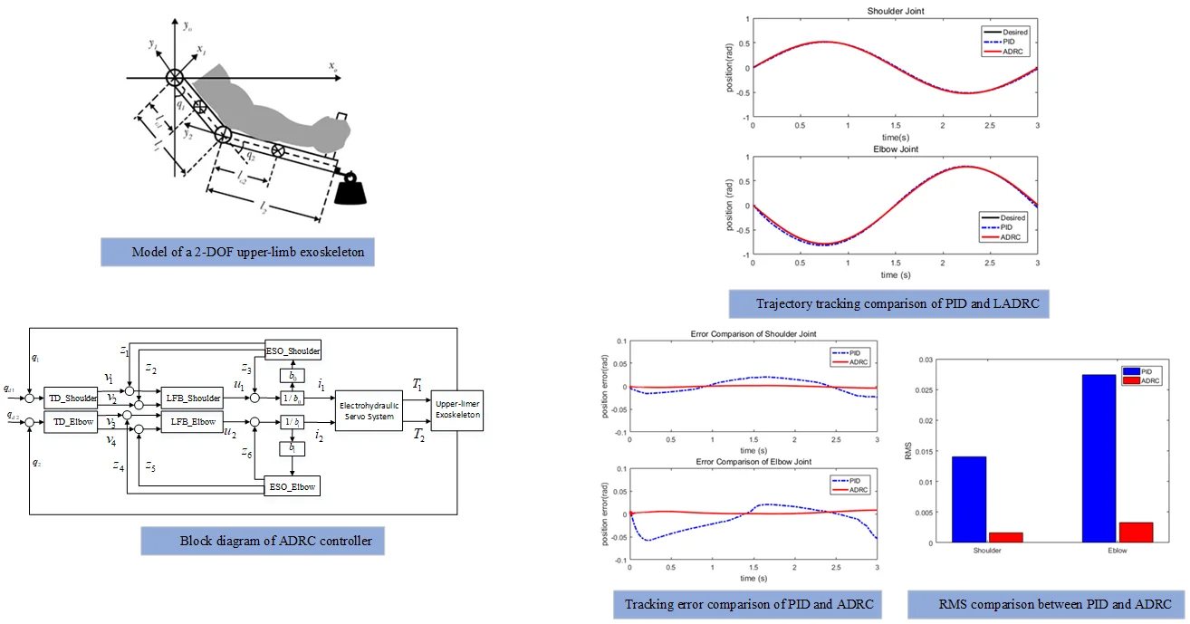
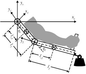
The exoskeleton is a typical human-robot collaboration system. The control systems of exoskeleton are different from the traditional robots, because the human operator is not the commander of the system, but also a part of the control loop. Hence, the human operator mainly makes the decisions, then the exoskeleton implements the tasks. A model of a 2-DOF upper-limb exoskeleton consisting of the load, the exoskeleton and an operator is shown in Fig. 1. The upper-limb exoskeleton has 2 DOFs, with the shoulder joint and elbow joint actuated and capable of following the rotations of the corresponding joints of the operator.
Without loss of generality, the dynamic equation of the upper-limb exoskeleton robot can be express as follows:
where is a vector of actuator joint torque; is a vector of exoskeleton angles for revolute joints; and are the joint velocities and accelerations respectively. is the total disturbances of the system. Meanwhile, is the inertia matrix, is the centripetal matrix, and is the gravity torque, respectively. , and denote the uncertainty of the robot system. The specific expression of the matrices , and can be described as:
where
where is the mass of the robotic upper arm, is the mass of the robotic forearm, is the length of the robotic upper arm, is the mass of external load, is the length of the robotic forearm, is the position of the center of the robotic upper arm, is the position of the center of the robotic forearm, is the inertia of the robotic upper arm and is the inertia of the robotic forearm.
Fig. 1Model of a 2-DOF upper-limb exoskeleton
Based on the dynamics model of robotic exoskeleton shown by Eq. (1), The system should be decoupled, and matrix can be approximated as . Assumption:
The mathematical model of robotic exoskeleton can be expressed as below:
The inertia matrix is symmetric positive definite, Eq. (4) can be rewritten as:
where, . is the total disturbance of the system, including system error, external disturbance and couple term. is the acceleration of the revolute joints.
2.2. Modeling of the electro-hydraulic servo system
The structure of EHSS is shown in Fig. 2. In many EHSS applications, valve dynamics is much faster than other parts of the system. Therefore, valve dynamics can be neglected, we assumed that the servo valve as a proportional block, by following approximation:
where is a positive electrical constant, and is the input current.
Fig. 2The structure of EHSS
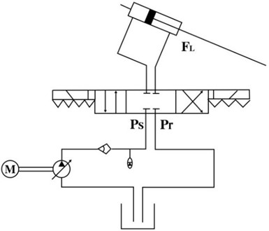
By applying the continuity law to each actuator chamber, the external leakage of EHSS is extremely small and can be neglected. The flow equation of actuator’s valve is described as:
where is the supplied flow rate to the forward chamber; is return flow rate of the return chamber. is the discharge coefficient; is the spool valve area gradient; is the density of hydraulic oil; is the supply pressure of the fluid; is the return pressure; is the head-side pressure; is the rod-side pressure; is defined as:
The pressure dynamics in actuator chambers can be described as:
where , are the control volumes of the actuator chambers; is the effective bulk modulus of the system; is the coefficient of the total internal leakage of the actuator due to the pressure; is the load pressure of the dynamic actuator. The actuated force can be express as:
where is the head-side area; is the rod-side area. is the bore diameter; is the rod diameter. As the rod diameter is small compared to the bore diameter, the can be simplified as:
The EHSS driving torque can be express as:
where is arm of torque.
For the 2-DOF upper-limb exoskeleton, two sets of EHSS generate the force to drive the robotic shoulder and arm respectively:
where and are the actuator torques of shoulder joint and elbow joint. and are the head-side pressure and rod-side pressure of shoulder joint. and are the head-side pressure and rod-side pressure of elbow joint. and are the arms of force for the robotic shoulder and elbow. Based on the geometry of robotic exoskeleton, the and can be calculated as:
where , , and are the geometric length of the upper limb exoskeleton. Fig. 3 provides the design geometry of the exoskeleton hydraulic cylinder.
The parameters of Electro-hydraulic Servo system are used in Table 1.
3. Control strategy design for upper-limb exoskeleton
The purpose of our upper-limb exoskeleton design is to evaluate the position tracking performance. To implement this goal, the desired position should be acquired. In this system, the desired angles for revolute joints for the test purposes are sinusoidal signals at a sampling frequency of 1000 Hz:
Fig. 3The design geometry of the exoskeleton hydraulic cylinder
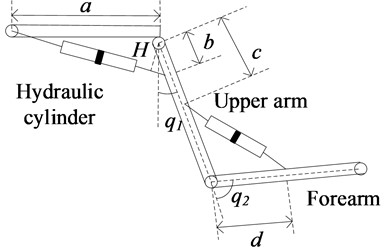
Table 1Parameters of EHSS
Parameter | Representation | Value |
Head-side area | 1.77×10⁻⁴ m2 | |
Rod-side area | 1.57×10⁻⁴ m2 | |
Bore diameter | 0.015 m2 | |
Rod diameter | 0.0075 m2 | |
Return pressure | 5×10⁴ Pa | |
Supply pressure of the fluid | 2×10⁶ Pa | |
Density of hydraulic oil | 830 kg m3 | |
Spool valve area gradient | 9.59×10⁻³ m2 | |
Effective bulk modulus of the system | 2×10⁷ Pa | |
Discharge coefficient | 0.61 | |
Coefficient of the total internal leakage | 8×10-12 M5N-1s-1 | |
Positive electrical constant | 1.38×10⁻⁴ m3s-1Pa-1 | |
Volume of the actuator chamber | 1.4×10⁻⁴ m3 | |
Volume of the actuator chamber | 1.4×10⁻⁴ m3 | |
Length of the robotic upper arm | 0.45 m | |
Length of the robotic forearm | 0.5 m |
3.1. Design PID controller for upper-limb exoskeleton
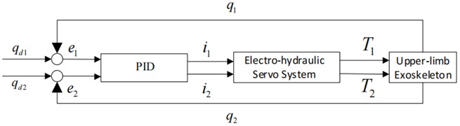
The conventional PID controller is widely adopt due to its simple structure and its gains can be easily tuned. The fixed PID controller of the hydraulically actuated exoskeleton system is shown in Fig. 4, and can be constructed as follows:
where (), () and () are proportional, integration and differential gains respectively. Moreover, and are the errors between the desired positions and actual positions.
Fig. 4Block diagram of PID controller
3.2. Design ADRC for upper-limb exoskeleton
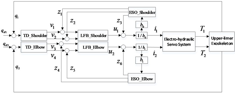
The ADRC method adopt nonlinear function, resulting in difficult analysis and parameter setting complex. Therefore, ADRC is designed based on the dynamic of robotic exoskeleton. In this paper, the dynamics model of the exoskeleton leg is multi-input and multi-output (MIMO) system. The Block diagram of ADRC controller is shown in Fig. 5. After system is decoupled, ADRC can be designed to control each joint respectively. Eq. (5) can be split into two independent equations for the shoulder and elbow joint as follow:
The ADRC controller consist three main parts, i.e., the tracking differentiator (TD) to provide derivative of the input signal, the extend state observer (ESO) to estimate the states and the disturbances and the nonlinear feedback to generate the control signal. TD is used to generate the arranged transition process and extract the input signal’s differential of each order. The tracking differentiator is designed in the form of:
where and are desired angles, and are the observer gains to ensure convergence of the error. ESO is designed to estimate and compensation total disturbances of hydraulically actuated exoskeleton system. Two extended state observers can be obtained as follows:
where , , and , , are the observer gains. The observations error are defined as , . For the purpose of tuning simplification, all the observer poles are placed at . The observer gains can be determined according to the characteristic polynomial [22]:
where is the bandwidth of observer and the gain vector can be expressed as follows: , , and , , . In this paper, the bandwidth of two observers is defined as the same values of . The bandwidth of feedback controller is defined as . Finally, the feedback control law in the proposed control can be written as follows:
where , and , are the proportional and differential gains, respectively.
Fig. 5Block diagram of ADRC controller
4. Simulation results
4.1. Selection of system parameters
The objectives of this section are to compare the tracking performance of PID control approach and the ADRC strategy. There are two ESOs to estimate existing disturbance for the shoulder joint and the elbow joint respectively. The parameters of the EHSS and the upper-limb exoskeleton are listed in Table 1. Two simulations are carried out, in MATLAB, by using PID control strategy and the ADRC. The parameters of ADRC are shown in Table 2, and are the amplification coefficients of and . is the bandwidth of observer, and the selection of its value affect the tracking effect.
Table 2Parameters for ADRC
Symbol | Value | Symbol | Value |
1 | 4 | ||
1200 | 3600 | ||
3600 | 4.32×10⁶ | ||
4.32×10⁶ | 1.728×10⁹ | ||
1.728×10⁹ | 160000 | ||
160000 | 800 | ||
800 |
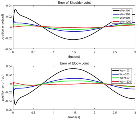
Fig. 6 shows the tracking error of each joint with different in proposed ADRC. As seen in the figure, the error decrease as the value of increases, the larger the value of is, the faster the errors converge.
Fig. 6Tracking error with different w0 in proposed ADRC
4.2. Comparisons of the conventional PID controller and ADRC controller
The system simulations are carried out, in MATLAB (Version R2016a), by using PID control strategy and ADRC approach presented in respectively. The parameters of the controllers are chosen using Ziegler and Nichols method [23]. Then, the optimum parameters for the PID controller can be provided as 240, 40, 180 and 200, 80, 120. The external disturbance is generated by a sinusoidal signal as follows:
Fig. 7Trajectory tracking comparison of PID and LADRC
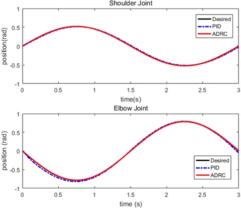
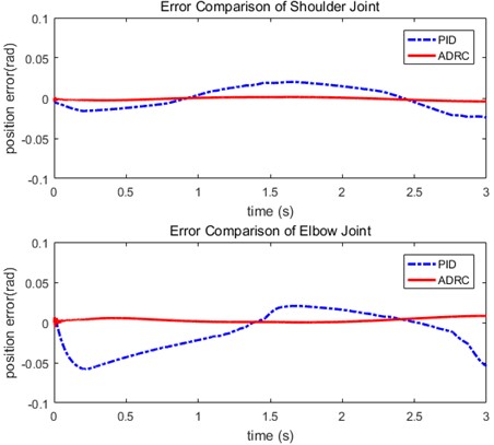
Performances of the conventional PD controller and ADRC method for position trajectory control are compared next. Figs. 7, 8 show trajectory tracking, position errors for each joint. As shown in the Fig. 7, The trajectories produced by the PID controller is depicted in red color, then ADRC is depicted in blue color, and the desired angle is depicted in black color. The performance of ADRC method is better compared to the conventional PID control. Fig. 8 shows the trajectory tracking error of the shoulder joint and the elbow joint respectively. It is seen that the deviations occur from the desired trajectory and ADRC controller produces better results than the conventional PID controller. The ADRC controller possess 3 ms lag, which is smaller than 11ms lag for the PID controller.
Fig. 8Tracking error comparison of PID and ADRC
To evaluate the performance of the general PID control approach and the proposed method, the tracking errors are compared. The tracking performances are indicated by root-mean-square (RMS) error [12]:
Fig. 9RMS comparison between PID and ADRC
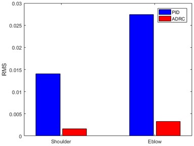
Fig. 9 provides the RMS errors of the human-machine position. From Fig. 9, both of the tracking errors of shoulder joint and elbow joint under the ADRC approach are smaller than those under the conventional PID control strategy. It is obviously to see that the proposed ADRC method is better than PID control with its robustness to external disturbance or un-modeled system dynamic, and it will be easy to implement.
5. Conclusions
The ADRC strategy for 2-DOF upper-limb exoskeleton, under the actuation of hydraulic, was explored in this paper. Considering the unavailability of precise model parameters and the uncertain disturbances in upper-limb exoskeleton actuated by EHSS. The proposed control strategies not only reduce the influence of unknown disturbances and eliminates the dependence on accurate model parameters, but also improve the tracking accuracy of the exoskeleton system and make the error converge quickly. The simulation results validate the effectiveness of the proposed method. The limitation of our approach is tuning the ADRC parameters automatically. In the future, the combination of ADRC with other model free tuning techniques will be investigated to reduce this limitation. It is proposed for the further development to investigate the robustness of ADRC for the external load uncertainty and motion velocity change. Moreover, Future work will include applying different types of other path tracking trajectories.
References
-
D. Calafiore, F. Negrini, N. Tottoli, F. Ferraro, O. Ozyemisci-Taskiran, and A. de Sire, “Efficacy of robotic exoskeleton for gait rehabilitation in patients with subacute stroke: a systematic review,” European Journal of Physical and Rehabilitation Medicine, Vol. 58, No. 1, pp. 1–8, Mar. 2022, https://doi.org/10.23736/s1973-9087.21.06846-5
-
A. Rodríguez-Fernández, J. Lobo-Prat, and J. M. Font-Llagunes, “Systematic review on wearable lower-limb exoskeletons for gait training in neuromuscular impairments,” Journal of NeuroEngineering and Rehabilitation, Vol. 18, No. 1, pp. 1–21, Dec. 2021, https://doi.org/10.1186/s12984-021-00815-5
-
C. Kandilakis and E. Sasso-Lance, “Exoskeletons for personal use after spinal cord injury,” Archives of Physical Medicine and Rehabilitation, Vol. 102, No. 2, pp. 331–337, Feb. 2021, https://doi.org/10.1016/j.apmr.2019.05.028
-
J. Kim et al., “Reducing the metabolic rate of walking and running with a versatile, portable exosuit,” Science, Vol. 365, No. 6454, pp. 668–672, Aug. 2019, https://doi.org/10.1126/science.aav7536
-
Z. Wang et al., “Study on the control method of knee joint human-exoskeleton interactive system,” Sensors, Vol. 22, No. 3, p. 1040, Jan. 2022, https://doi.org/10.3390/s22031040
-
Z. Li, B. Huang, Z. Ye, M. Deng, and C. Yang, “Physical human-robot interaction of a robotic exoskeleton by admittance control,” IEEE Transactions on Industrial Electronics, Vol. 65, No. 12, pp. 9614–9624, Dec. 2018, https://doi.org/10.1109/tie.2018.2821649
-
W. Cao et al., “A lower limb exoskeleton with rigid and soft structure for loaded walking assistance,” IEEE Robotics and Automation Letters, Vol. 7, No. 1, pp. 454–461, Jan. 2022, https://doi.org/10.1109/lra.2021.3125723
-
X. Zhang, G. Wang, P. Yuan, H. Xu, and Y. Hou, “A control strategy for maintaining gait stability and reducing body-exoskeleton interference force in load-carrying exoskeleton,” Journal of Intelligent and Robotic Systems, Vol. 97, No. 2, pp. 287–298, Feb. 2020, https://doi.org/10.1007/s10846-019-01043-9
-
N. Zhou, Y. Liu, Q. Song, and D. Wu, “A compatible design of a passive exoskeleton to reduce the body-exoskeleton interaction force,” Machines, Vol. 10, No. 5, p. 371, May 2022, https://doi.org/10.3390/machines10050371
-
Song, Lee, Park, and Baek, “Design and performance of nonlinear control for an electro-hydraulic actuator considering a wearable robot,” Processes, Vol. 7, No. 6, p. 389, Jun. 2019, https://doi.org/10.3390/pr7060389
-
C. Yang, Q. Huang, and J. Han, “Decoupling control for spatial six-degree-of-freedom electro-hydraulic parallel robot,” Robotics and Computer-Integrated Manufacturing, Vol. 28, No. 1, | pp. 14–23, Feb. 2012, https://doi.org/10.1016/j.rcim.2011.06.002
-
J. Tang, J. Zheng, and Y. Wang, “Direct force control of upper-limb exoskeleton based on fuzzy adaptive algorithm,” Journal of Vibroengineering, Vol. 20, No. 1, pp. 636–650, Feb. 2018, https://doi.org/10.21595/jve.2017.18610
-
L. Teng, M. A. Gull, and S. Bai, “PD-based fuzzy sliding mode control of a wheelchair exoskeleton robot,” IEEE/ASME Transactions on Mechatronics, Vol. 25, No. 5, pp. 2546–2555, Oct. 2020, https://doi.org/10.1109/tmech.2020.2983520
-
W. Sun, J.-W. Lin, S.-F. Su, N. Wang, and M. J. Er, “Reduced adaptive fuzzy decoupling control for lower limb exoskeleton,” IEEE Transactions on Cybernetics, Vol. 51, No. 3, pp. 1099–1109, Mar. 2021, https://doi.org/10.1109/tcyb.2020.2972582
-
M. Torabi, M. Sharifi, and G. Vossoughi, “Robust adaptive sliding mode admittance control of exoskeleton rehabilitation robots,” Scientia Iranica, Oct. 2017, https://doi.org/10.24200/sci.2017.4512
-
C. Dai, J. Yang, Z. Wang, and S. Li, “Universal active disturbance rejection control for non‐linear systems with multiple disturbances via a high‐order sliding mode observer,” IET Control Theory and Applications, Vol. 11, No. 8, pp. 1194–1204, May 2017, https://doi.org/10.1049/iet-cta.2016.0709
-
J. Li, Y. Xia, X. Qi, and P. Zhao, “Robust absolute stability analysis for interval nonlinear active disturbance rejection based control system,” ISA Transactions, Vol. 69, pp. 122–130, Jul. 2017, https://doi.org/10.1016/j.isatra.2017.04.017
-
Y. Huang and J. R. Wang, “Optimized linear active disturbance rejection controller design for hydraulic turbine governing system,” Journal of System Simulation, Vol. 28, No. 12, pp. 3033–3040, 2016.
-
S. N. Pawar, R. H. Chile, and B. M. Patre, “Modified reduced order observer based linear active disturbance rejection control for TITO systems,” ISA Transactions, Vol. 71, pp. 480–494, Nov. 2017, https://doi.org/10.1016/j.isatra.2017.07.026
-
L. Sun, Q. Hua, D. Li, L. Pan, Y. Xue, and K. Y. Lee, “Direct energy balance based active disturbance rejection control for coal-fired power plant,” ISA Transactions, Vol. 70, pp. 486–493, Sep. 2017, https://doi.org/10.1016/j.isatra.2017.06.003
-
L. Zhao, B. Zhang, H. Yang, and Q. Li, “Optimized linear active disturbance rejection control for pneumatic servo systems via least squares support vector machine,” Neurocomputing, Vol. 242, pp. 178–186, Jun. 2017, https://doi.org/10.1016/j.neucom.2017.02.069
-
Qing Zheng, Lili Dong, Dae Hui Lee, and Zhiqiang Gao, “Active disturbance rejection control for MEMS gyroscopes,” in 2008 American Control Conference (ACC ’08), pp. 4425–4430, Jun. 2008, https://doi.org/10.1109/acc.2008.4587191
-
J. G. Ziegler and N. B. Nichols, “Optimum settings for automatic controllers,” Journal of Dynamic Systems, Measurement, and Control, Vol. 115, No. 2B, pp. 220–222, Jun. 1993, https://doi.org/10.1115/1.2899060
Cited by
About this article

This work was supported by Key Research and Development Plan of Hubei Province (2021BGD013), Hubei University of Technology Ph.D. Research Startup Fund Project (BSQD2020014) and Science and Technology Research Program of Hubei Provincial Department of Education (T201805).
The datasets generated during and/or analyzed during the current study are available from the corresponding author on reasonable request.
Jing Tang: application of statistical, mathematical and computational, to synthesize study data. conducting a research and investigation process, specifically performing the experiments and data collection. Jiaxun Cao: Preparation and presentation of the published work by those from the original research group. Minghu Wu: management and coordination responsibility for the research activity planning and execution. Lun Zhao: preparation and presentation of the published work, specifically data presentation. Fan Zhang: software development; designing computer programs; implementation of the computer code and supporting algorithms.
The authors declare that they have no conflict of interest.
