A method of sound source recognition based on tow weak selection compressed sensing

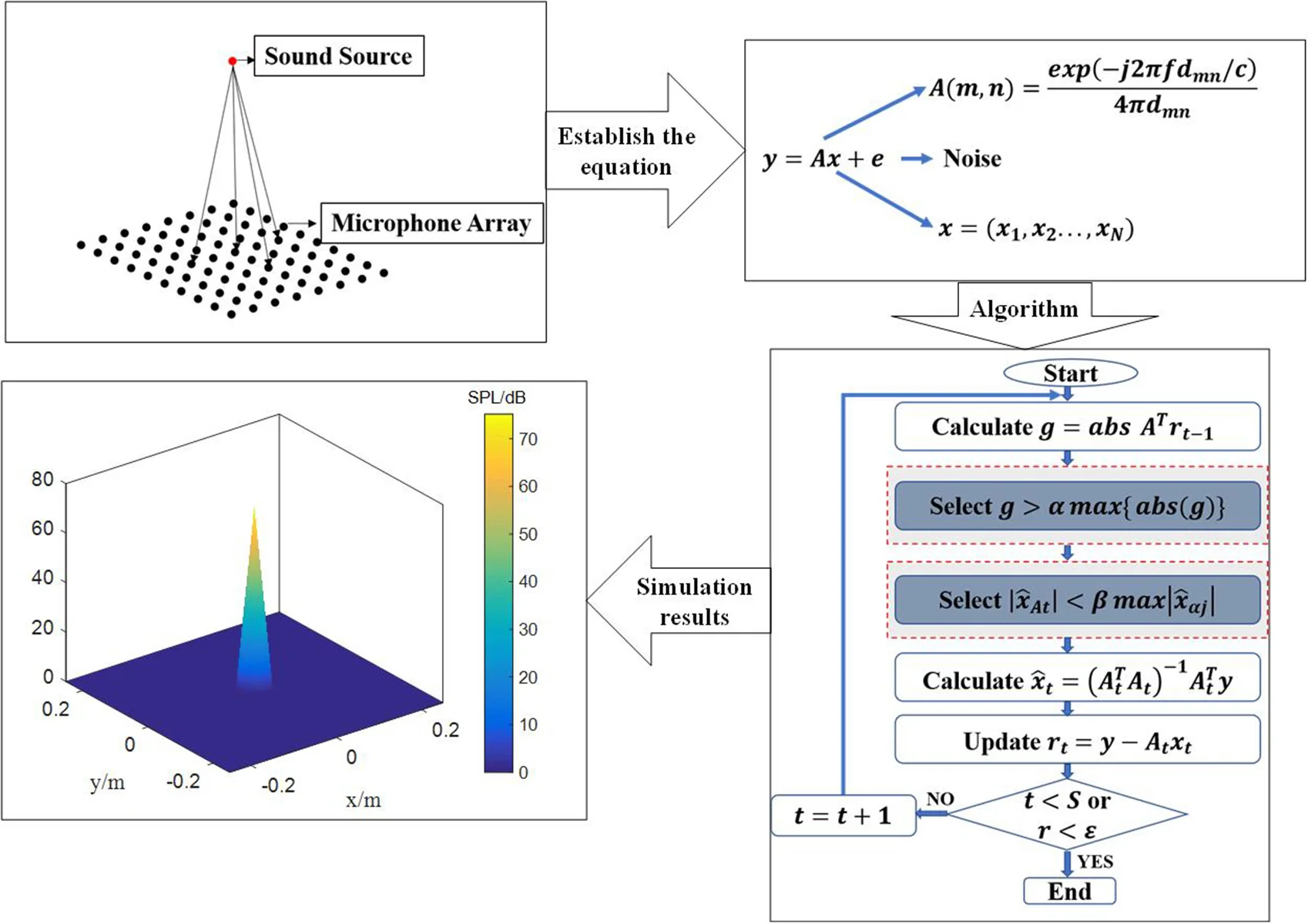
2.1. The acoustic field model

Assuming that the array is planar, the total number of microphones in the array are $M$, and the frequency of the sound source is $f$, the sound source surface is divided into grid nodes with the same number of row and column nodes, and there are a total of $N$ grid nodes. The distance from the m microphone to the n grid node is denoted as $d_{mn}$ ($m$= 1, 2... $M$, $n$= 1, 2... $N$). According to the Helmholtz integral equation of the free field Green’s function [12], the transfer matrix between the microphone array and the sound source plane node is established, as shown in below Eq. (1):

where $c$ is the speed of sound, ${\bar{p}}_m$ is the coordinate of the m microphone, $p_n$ is the coordinate of the $n$ grid node. Assume that the sound source signal located on the sound source plane can be expressed as $x=(x_1,x_2...,x_N)$, then the microphone measurement value can be expressed as $y=Ax$. However, there is some noise in the practical application environment, so the measured value of the microphone is expressed as $y=Ax+e$, where $e$ represents noise.

2.2. Reconstruction algorithm

The goal of compressed sensing theory is to reconstruct signal $X$ of sparse sound source by measurement value $Y$ and measurement matrix $A$. The above problem is to solve the underdetermined linear equations, which usually have multiple solutions, owing to $M\le N$. When $x$ is a sparse sound source signal, solving $x$ can be regarded as the process of seeking the sparsiest solution, which is the process of solving the $l_0$ norm. However, this is a NP-hard problem, which is usually difficult to calculate. In order to solve this problem, Candes and Donoho et al. [13] proposed the idea of replacing $l_0$ norm with $l_1$ norm, so the problem can be expressed as a constraint problem in below Eq. (3), where $\epsilon$ is determined by the given noise:

Donoho et al. have shown that the solution of $l_0$ norm and the solution of $l_1$ norm are approximately equal under RIP. Greedy tracking algorithm, as a method of compressed sensing reconstruction algorithms, has been widely concerned and researched due to its high reconstruction efficiency and precision. The main algorithms include orthogonal matching pursuit (OMP) [14], stagewise orthogonal matching pursuit (STOMP) [15] and SWOMP [16], where SWOMP has a good performance in terms of complexity and precision. The SWOMP algorithm iterates to the final result by removing the wrong atoms from the set of atoms using a threshold.

3.1. Basis of two choices

In the compressed sensing reconstruction algorithm, the SWOMP simplifies OMP and improves the calculation speed. However, the atoms obtained in each iteration are not the best representation of the signal, which leads to a decrease in the reconstruction precision. In practice, the accuracy of the reconstructed signal is far inferior to that of OMP. In addition, the SWOMP can accurately reconstruct the original signal only when the sparsity of the signal is correctly estimated.

To solve the above problems, literature [17, 18] proposed an improved algorithm that relied too heavily on the sparsity, which selected the initial atomic set through the piecewise weak selection criteria, then tested the reliability of the previously selected atoms, and deleted the previously selected wrong atoms from the current atomic set, so as to obtain the final result through iteration. In this paper, the TSWOMP compressed sensing sound source reconstruction algorithm is proposed, which can make the algorithm no longer need the accurate information of sparsity with higher reconstruction accuracy and lower complexity. Ideally, the estimate of the result of the previous step should be greater than the estimate of the result of this step. If, in the process of an iteration, the estimated value of the result obtained according to the first piecewise weak selection criterion is much smaller than the estimated value of the result obtained before, it is very likely that the wrong atom was selected in the previous selection. Therefore, it is necessary to design a "second segmenting weak selection" standard to remove the previously selected wrong atoms from the current atom support set. The second weak selection parameter number $\beta \in \left(\mathrm{0,1}\right)$ is introduced, and the second piecewise weak selection criterion is shown in Eq. (4):

where $d\in D$, $D$ is the index of the deleted set of the second weak selection, ${\widehat{\theta }}_{At}$ and ${\widehat{\theta }}_{\alpha j}$ is the results obtained before and after the first piecewise weak selection in the $t$-th iteration, respectively.

3.2. TSWOMP algorithm specific steps

According to SWOMP and the above theoretical analysis, the specific steps of TSWOMP are obtained. The sound source signal $x$ can be obtained by sensing matrix $A$ and measuring signal $y$.

Input: $M\times N$ sensor matrix $A$, $N\times 1$ dimensional observation vector, Number of iterations $S=$10, threshold parameter $\alpha =$0.8 and $\beta =$0.6.

Output: signal estimation $\widehat{x}$, residual $r_S=y-A_S{\widehat{x}}_S$.

Step 1: Initialization $r_0=y$, ${\mathrm{\Lambda }}_0=\varnothing$, $A_0=\varnothing$, $t=1$.

Step 2: Calculate $g=\mathit{abs}\left(A^T{r}_{t-1}\right)$, select the values in $g$ greater than the threshold $Th=\alpha \mathit{max}\{abs\left(g\right)\}$, and form the set $J_0$ with the corresponding column number $J$ of $A$.

Step 3: Make ${\mathrm{\Lambda }}_t={\mathrm{\Lambda }}_{t-1}\cup J_0$, $A_t=A_{t-1}\cup a_j$, if ${\mathrm{\Lambda }}_t={\mathrm{\Lambda }}_{t-1}$ (no new atoms are selected), then the iteration is stopped and step 8 is entered.

Step 4: Find the least squares solution of $y=A_t{x}_{At}$ and $y=a_j{x}_{\alpha j}$, and delete the values that satisfy $\left|{\widehat{x}}_{At}\right|<\beta \mathit{max}\left|{\widehat{x}}_{\alpha j}\right|$, the column number of these values corresponding to $A$ is $D$, update ${\mathrm{\Lambda }}_t={\mathrm{\Lambda }}_t\backslash D$ and $A_t$.

Step 5: Find the least squares solution of$y=A_t{x}_t:{\widehat{x}}_t=\mathit{argmin}‖y-A_t{x}_t‖={\left(A_t^T{A}_t\right)}^{-1}{A}_t^{T}y$.

Step 6: Update the residual $r_t=y-A_t{\widehat{x}}_t=y-{\left(A_t^T{A}_t\right)}^{-1}{A}_t^{T}y$.

Step 7:$t=t+1$. If $t<S$ then return to Step 2. If $t>S$ or $r_t$ reaches precision, enter Step 8.

Step 8: The $\widehat{x}$ obtained by the reconstruction has a non-zero term at ${\mathrm{\Lambda }}_t$, and the results are ${\widehat{x}}_t$ obtained by the last iteration respectively, and the rest positions are 0.

3.3. Numerical simulation

In order to verify the feasibility and advantages of the proposed method, the following simulation process adopts CBF, SWOMP and TSWOMP respectively. Based on the simulation results, the influence of frequency and signal-to-noise ratio on sound source localization is analyzed, and the accuracy of sound source identification is analyzed. It is assumed that the sound source is located on the measuring surface, its coordinate is (0, 0, 0), the dynamic range of the sound pressure level is 30 dB, an 8×10 microphone array is adopted, the grid points on the sound source surface are 21×21, the grid spacing is 0.025 m, and the distance from the microphone array to the sound source surface $z=$ 0.25 m.

After several simulations, TSWOMP can obtain a better reconstruction effect when the weak selection parameters $\alpha$ and $\beta$ are 0.5-1, so this simulation takes $\alpha =$0.6 and $\beta =$0.8. The threshold parameter of SWOMP is set as $\alpha =$0.9. The number of iterations is set as $L=$10.

3.4. The influence of frequency on identification results

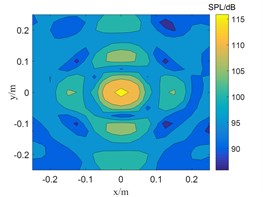
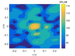
The CBF, SWOMP and TSWOMP are used to locate and simulate the sound source at the frequency of 800 Hz and 2500 Hz respectively, and the SNR was 30 dB. The results are shown in Fig. 1 and Fig. 2.

Fig. 1The location results of 800 Hz sound source

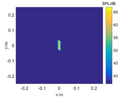
a) TSWOMP

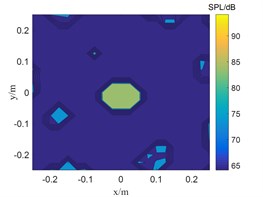
b) SWOMP

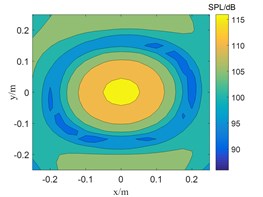
c) CBF

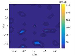
Fig. 2The location results of 2500 Hz sound source

a) TSWOMP

b) SWOMP

c) CBF

The frequency in Fig. 1 is 800 Hz, and the CBF, SWOMP and TSWOMP can accurately locate the location of the sound source, but there is a large error between the sound pressure values identified by the three algorithms and the sound source pressure values. The main lobe width of CBF and SWOMP are much larger than that of TSWOMP. It can be seen that TSWOMP can effectively reduce the main lobe width, suppressing the influence of side lobe, and significantly improve the resolution at low frequency. The frequency in Fig. 2 is 2500 Hz, and TSWOMP can accurately locate the location and sound pressure of the sound source. The CBF localization results of the main lobe width are much larger than the other two algorithms. Although SWOMP can reduce the width of the main lobe, there are many side lobes and pseudo sound sources, and there is a large error between the recognized sound pressure value and the sound source value. By comparing Fig. 1 and Fig. 2, it is found that with the decrease of frequency, TSWOMP has a certain recognition error in the case of low frequency.

3.5. The influence of SNR on recognition results

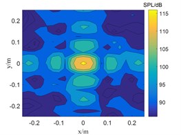
A sound source with a frequency of 5000 Hz, the SNR of 15 dB and 0 dB, and a distance of 0.25m from the array to the measuring surface was selected. The CBF, SWOMP and TSWOMP were used for simulation experiments. The results are shown in Fig. 3 and Fig. 4.

Fig. 3The localization results of when sound source the SNR is 15 dB

a) TSWOMP

b) SWOMP

c) CBF

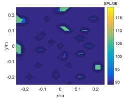
Fig. 4The localization results of when sound source the SNR is 0 dB

a) TSWOMP

b) SWOMP

c) CBF

The SNR is 15 dB in Fig. 3, and the sound pressure identified by CBF and SWOMP has a large error with the sound source pressure value, while TSWOMP can accurately identify the sound source location and sound source pressure value. Compared with CBF and SWOMP, TSWOMP has smaller main lobe width, eliminating the influence of side lobe, and reducing the error of sound pressure value reduction. By comparing Fig. 3 and Fig. 4, it can be seen that with the reduction of SNR, CBF and SWOMP are greatly affected by noise, where the main lobe width becomes larger, and the number of side lobes in positioning results increases. However, TSWOMP can effectively reduce the main lobe width, suppressing the influence of side lobes, and improve the accuracy of sound pressure identification of sound source the low SNR.

3.6. Accuracy analysis of identification results

In order to verify the accuracy of TSWOMP recognition results, a frequency of 6500 Hz, a signal to noise ratio of 30 dB, and a distance of 0.25 m from the array to the measuring surface of 100 arbitrary sound sources were taken, then TSWOMP and SWOMP were used for simulation experiments. The results are shown in Fig. 5.

Fig. 5The result of localization any 100 sound sources

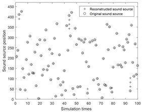
a) TSWOMP

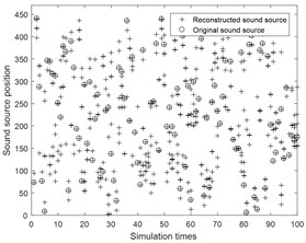
b) SWOMP

Fig. 5 shows that the recognition rate of TSWOMP algorithm is significantly higher than that of SWOMP algorithm. When the grid spacing is 0.025 m, TSWOMP can accurately identify the sound source location. However, the error caused by noise leads to sidelobe in the recognition result. After identifying 2000 random source positions, the sidelobe free probability of TSWOMP algorithm is about 94.8 %.