Application of A* algorithm in intelligent vehicle path planning

2.1. Dijkstra algorithm

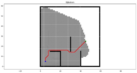
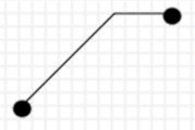
Dijkstra algorithm was proposed by Johnson in 1973 [4]. Dijkstra algorithm is mostly used for solving the shortest distance from one vertex to other vertices in the entitled graph. The algorithm stores the shortest distance from the starting point to each vertex through the array 𝐷 and the vertices corresponding to the shortest path that has been traversed through the set 𝑇. When executing the algorithm, the vertex with the smallest distance from the starting point is found from the vertices outside the set 𝑇 each time by iteration, and that point is added to the set 𝑇, and the values in the array 𝐷 are refreshed by that point until the set 𝑇 contains all vertices. The Dijkstra algorithm is shown schematically in Fig. 1.

Fig. 1Dijkstra’s algorithm diagram

2.2. Breadth-first-search (BFS)

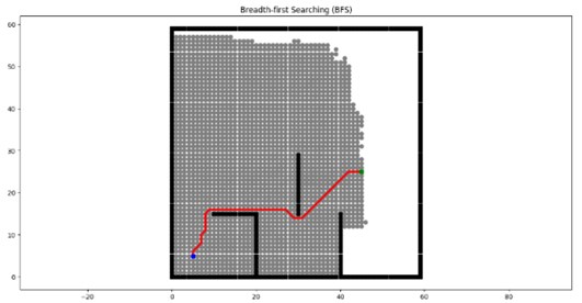
The breadth-first search algorithm is a heuristic search algorithm [5], which references an estimation function by which the estimated value of the current node to the target node is calculated in path planning, and then the node with the smallest estimated value is selected to be visited, and so on until the target node is searched. The best-first search algorithm has improved search efficiency compared to Dijkstra's algorithm, but it cannot determine whether a shortest path can be found.

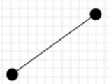
The breadth-first search algorithm is efficient computationally when searching for a path, but it is uncertain whether an optimal path can be found because only the estimated value from the current node to the target node is taken into account. The schematic diagram of the best-first search algorithm is shown in Fig. 2.

Fig. 2BFS algorithm diagram

3.1. Principle of A* algorithm

The A* algorithm is a heuristic search algorithm that combines the respective features of Dijkstra's algorithm and BFS (Breath-First Search) algorithm. It has better accuracy and flexibility to ensure that the intelligent vehicle obtains the optimal path while maintaining the efficiency of path search as much as possible. The core part of the algorithm lies in the design of the estimation function [6], and the general form of the estimation function of the A* algorithm is Eq. (1):

where $f\left(n\right)$ is the cost estimate from the initial state to the target state via state $n$, $g\left(n\right)$ is the actual cost from the initial state to state $n$, and $h\left(n\right)$ is the estimated cost of the best path from state n to the target state, also known as the heuristic function.

If the value of $h\left(n\right)$ is low, the algorithm can obtain the shortest path, but the search operation is slow. If the value of $h\left(n\right)$ is high, the search speed of A* algorithm will become faster, but the obtained path is not the optimal path [7]. Manhattan distance, Euclidean distance, Chebyshev distance, etc. are often used as heuristic functions in practical calculations [8]. For any two points A and B in a two-dimensional right-angle coordinate system the coordinates of the two points are ($X_A,Y_A)$, ($Y_B,Y_B$) then the three distance functions are.

(1) Manhattan distance is the sum of the absolute value of the difference between the $X$ and $Y$ coordinates of two points A and B located in the coordinate system:

(2) Chebyshev distance is a metric in vector space, which is the maximum value obtained by comparing the difference between the horizontal and vertical coordinates between two points A and B, respectively, and then taking the absolute value, i.e.:

(3) Euclidean distance is the shortest linear distance between two points A and B located in the coordinate system, i.e.:

Fig. 3Three distance diagram

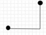
a) Manhattan distance

b) Diagonal distance

c) Euclidian distance

A detailed representation of the three distances is given in Fig. 3.

Compare by three distances, Manhattan distance is simple to calculate and efficient in path planning, but the quality of the planned path is poor; Euclidean distance is the shortest and easy to get the shortest path, but the calculation is complicated leading to low solution efficiency; diagonal distance as a heuristic function is relatively simple to calculate and the valuation error of path planning is small, so the diagonal distance heuristic function is used in this paper.

The A* algorithm is to evaluate each node by the estimation function to get the optimal node, and repeat the process until the target node is searched. The algorithm steps are as follows.

1) Initialize the program and generate the environment map boundary, starting and target points and obstacles.

2) Add the starting point S to the OPEN table.

3) Judge whether the OPEN table is empty, if it is empty, the algorithm is finished and the path cannot be found, otherwise go to the next step.

4) Find the node N with the smallest $f\left(n\right)$ from the OPEN table, add it to the CLOSE table, and judge whether the node is the target node E. If it is the target node E, the algorithm ends, otherwise go to the next step.

5) Find all neighboring nodes $X_i$ of node N ($i<k$, $k$ is the number of all nodes adjacent to node N). If $X_i$ is not in the OPEN table nor in the CLOSE table, calculate and add it to the OPEN table; if $X_i$ is in the OPEN table, but smaller than the estimated value in the OPEN table, update the estimated value in the OPEN table and sort it from smallest to largest; if $X_i$ is in the CLOSE table, ignore the point.

6) Over-cycle the algorithm until the target point E is in the CLOSE table, indicating that the optimal path has been found, or the OPEN table is empty, and the algorithm ends.

After running this algorithm, the target node will point to its leading node, with so on, until the leading of a node is the starting node, and the global optimal path can be obtained.

3.2. Deficiencies of the A* algorithm

The analysis above shows that although the A* algorithm is simple in principle and convenient to use, however, the algorithm needs to continuously update the OPEN array list and CLOSE array list during the search process to calculate the estimated value of each node, thereby finding the minimum node of the optimal path, thus also revealing that the A* algorithm has certain deficiencies.

(1) the impact of the heuristic function on the algorithm. Heuristic function in the A* algorithm, play a guiding role in the path search, the effect of its role is good or bad, directly determine the efficiency of the path search, but the traditional heuristic function will have some inefficiency, which leads to the efficiency of the path search is not high.

(2) There are too many unnecessary inflection points in the planned path, which leads to poor smoothness and increased danger, which is not conducive to smart cars driving in the actual environment.

4.1. Optimization of the heuristic function $\mathit{h}\left(\mathit{n}\right)$

The traditional heuristic function will have some problems of low efficiency, in order to address this problem， this paper introduces the weight coefficient $w\left(n\right)$ on the basis of the original heuristic function, and the improved heuristic function:

In Eq. (5), $w\left(n\right)$ is the weight coefficient of the heuristic function $h\left(n\right)$. Adding this weight coefficient can make the search of the heuristic function more efficient. When it is far from the target point, the weight coefficient of $w\left(n\right)$ is larger, which can accelerate the algorithm to search toward the target point, and when it is close to the target point, the weight coefficient of $w\left(n\right)$ is smaller, which can make the algorithm search for a more accurate path. by using the optimized heuristic function can greatly improve the efficiency of intelligent vehicle path planning.

4.2. Path smoothing

When using the A* algorithm for path search, there are many inflection points and redundant points because of the angle limitation. To address this problem, this paper uses the Floyd algorithm [9] to smooth the paths and remove the redundant inflection points, thus making the paths smoother and also shortening the time loss of smart cars at the inflection points to improve the global path planning efficiency.

Floyd algorithm, also known as the interpolation method, is an algorithm for finding the shortest path between multiple source points in a given weighted graph, drawing on the idea of dynamic programming. Combining the A* algorithm with the Floyd algorithm, the iterative optimization of the nodes by the Floyd algorithm results in an increase in the smoothness of the planned path compared to the path using only the A* algorithm, while shortening the length of the path, which is beneficial to the global path planning of smart cars in the real environment. The schematic diagram of the Floyd algorithm [10] is shown in Fig. 4.

Fig. 4Floyd algorithm schematic

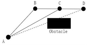
$L\left(A,D\right)$ is the distance from node A to node D and $R\left(A,D\right)$ is the path from node A to node D. From Fig. 4, it can be seen that there are obstacles between nodes A and D. Suppose $L\left(A,D\right)=+\infty$, the distance between nodes A and D is infinite. $R\left(A,D\right)=A\to D$, the path from node A to node D is node A pointing to node D.

Node B is the node planned to circumvent the obstacle between nodes A and D.

If:

Then:

Insert node C between nodes B and D.

If:

Then:

The original planned path is optimized by Floyd's algorithm and updated from nodes A, B and D to the current nodes A, C and D. The turning angle of the path is significantly reduced, thus making the smoothness of the path planning significantly improved, which can ensure smoother operation of the intelligent vehicle.

5.1. Creation of the simulation verification environment

The map modeling of the motion environment in which the intelligent vehicle is located is generally performed before the path planning. Depending on the type of map, the grid method, topological map method and free space method are commonly used [11]. Grid method is commonly used by the A* algorithm for path planning [12]. The basic idea of the grid method is to partition the environment region into a grid of the same size, each grid corresponds to a sub-partition of the real environment, and the grid map can characterize the initial and target locations of the smart car, the boundaries and obstacle areas within the environment region.

The environment modeling is based on MATLAB2021a platform. Firstly, the environment region is partitioned into $N\times N$ equal partitioned grids, which are described in MATLAB. An example of a 30×30 grid environment model built with MATLAB is shown in Fig. 5. The obstacle area is filled with black squares, yellow squares represent the starting point, and blue squares represent the target point.

Fig. 530×30 grid map

5.2. Experimental analysis

In order to verify the effectiveness of the improved A* algorithm, the simulation software platform MATLABR2021a is used to conduct simulation experiments and establish a raster environment map with a 20×20 grid, set the proportion of two obstacles in the grid environment map to 20 % and 40 % respectively, and randomly generate the starting and ending coordinates. The path planning is performed in the grid map using the traditional A* algorithm and the improved A* algorithm.

Fig. 6 and Fig. 8 show the results of searching with the traditional A* algorithm on the 20 % and 40 % random obstacle maps, respectively, and Fig. 7 and Fig. 9 show the results of searching with the improved A* algorithm on the 20 % and 40 % obstacles, respectively.

Fig. 620 % barrier traditional A* algorithm pathfinding results

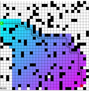
Fig. 720 % barrier improvement A* algorithm pathfinding results

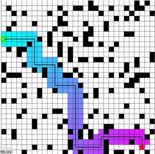
Fig. 840 % barrier traditional A* algorithm pathfinding results

Fig. 940 % barrier improvement A* algorithm pathfinding results

Comparing Fig. 6 and Fig. 7, Fig. 8 and Fig. 9, we can see that the paths are planned with the same starting point and target point in the obstacle map with the same occupancy ratio. It can be seen that the improved A* algorithm has a significant decrease in the number of search nodes and a certain degree of reduction in the number of inflection points compared with the traditional A* algorithm path finding results, so this paper improves the A* algorithm, which has a good effect in reducing the number of search nodes and the number of inflection points.

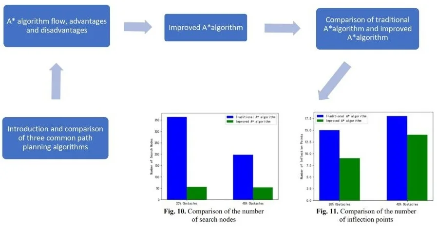
Fig. 10Comparison of the number of search nodes

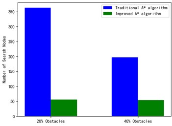
Fig. 11Comparison of the number of inflection points

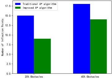
In order to more intuitively show the advantages of the improved A* algorithm in the entire path planning, the number of search nodes and the number of inflection points in the search path are reduced, and the results are shown in Fig. 10 and Fig. 11.

From Fig. 10 and Fig. 11, it can be seen that the improved A* algorithm proposed in this paper has a significant reduction in the number of search nodes and the number of inflection points compared with the traditional A* algorithm. Therefore, the improved A* algorithm of this paper for path planning of smart cars has good results in both reducing the number of search nodes and reducing the number of turns in the search path.