Path tracking with minimum time of vehicle handling inverse dynamics based on adaptive gauss pseudospectral method

2.1. Mathematical model of vehicle path tracking with minimum time problem

It is assumed that the longitudinal force acting on the front wheels is small, and the influence on the tire cornering characteristics affected by tangential ground force is ignored with tire cornering characteristics within the linear range. The 4-DOF vehicle model is depicted in Fig. 1 [16].

Fig. 14-DOF vehicle model

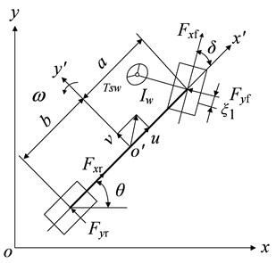
In the state-space form, the formula is as follows:

The parameters and corresponding definitions are shown in Table 1.

The lateral forces of the front and rear tires are:

where $k_2$ is the synthesized stiffness of rear tires, $\mu$ is the friction coefficient.

Taking the effect of the longitudinal load transfer on the front and rear axles into account, the vertical forces of the front and rear wheels are:

where $h_g$ is the height of the center of gravity.

The vehicle velocity in the body coordinate is projected in the Earth coordinate defined by $x$ and $y$ as:

According to Eq. (1) and Eq. (4), the state equation can be described as:

where $x\left(t\right)$ and $z\left(t\right)$ are the states and the input which are denoted respectively as $x\left(t\right)={\left[u\left(t\right),v\left(t\right),\omega \left(t\right),\delta \left(t\right),p\left(t\right),x\left(t\right),y\left(t\right),\theta \left(t\right)\right]}^T$, $z\left(t\right)=\left[T_{sw}\right(t){]}^T$.

2.2. Constrains

The constraints of initial and terminal states are:

In order to avoid pitch and yaw of the vehicle, the path constraint is [17]:

where $D$ is the wheel base, $K$ is the stability factor.

The constraints on $F_{xf}$, $F_{xr}$ are imposed when the vehicle is driven by the front wheels [18]:

When all the wheels are assumed as lock-braking, the constraints on $F_{xf}$, $F_{xr}$ can be rewritten in the following manner:

The boundary constraint is:

where $z_{min}$ and $z_{max}$ are the lower and upper limit values of the steering torque.

2.3. Optimal control object of path tracking problem

The minimum time problem of path tracking can be regarded as the optimal control problem in the control theory. The control target is to control the control variables to ensure the vehicle passing the given path within the minimum time. Therefore, the minimum time performance indicator is [19]:

where $t_0$ and $t_f$ are the initial and final time.

3.1. Continuous Bolza type problem

The minimum time optimal control problem can be treated as a Bolza problem [16].

The Bolza cost function is:

where $t_0$ and $t_f$ are the initial and final time, $\mathbf{x}\left(t\right)\in {\mathbf{R}}^n$, $\mathbf{z}\left(t\right)\in {\mathbf{R}}^m$.

The dynamic and boundary constraints as well as inequality path constraint are:

In Eqs. (13)-(16), the function $\psi$, $g$, $f$, $\phi$ and $C$ are defined as follows:

The indirect method transforms the above Bolz problem into a Hamiltonian boundary problem by introducing the Hamiltonian function based on the Ponte Liya maximum principle. The Hamiltonian function is defined as:

The optimal trajectories of the whole state variables and control variables can be obtained by solving a two-point boundary value problem composed of Hamiltonian equations, boundary conditions and path constraints.

3.2. AGPM

Gaussian pseudo-spectral method (GPM) separates the state variables and control variables on a series of collocations, and then uses the Lagrangian interpolation basis function to approximate the state variables and control variables with the discrete points as nodes. The derivative of the state variable to time can be approximated by deriving the global interpolation polynomial. The integral term in the performance index can be approximated by the Gaussian integral formula with high accuracy. The terminal state is obtained by integral of the initial state and the right function. After the above numerical approximation, the continuous optimal control problem can be transformed into a discrete nonlinear programming problem under a series of algebraic constraints.

GPM takes the K-order Legendre-Gauss point and the beginning and ending points as nodes to constitute $K+1$ Lagrangian interpolation polynomials. So the state and control variables can be approximated as [20]:

where $L_i\left(\tau \right)$ is Lagrange interpolating polynomials, $\mathbf{x}\left({\tau }_i\right)=\mathbf{X}\left({\tau }_i\right)$, $\mathbf{z}\left({\tau }_i\right)=\mathbf{Z}\left({\tau }_i\right)$.

For the state variable approximation Eq. (18), the kinetic differential constraint equation can be transformed into the following algebraic constraint:

where $\mathbf{D}\in {\mathbf{R}}^{n\times (n+1)}$.

The interpolation nodes in GPM include $N$ LG points, ${\tau }_1,{\tau }_2\cdots ,{\tau }_N$, the initial point ${\tau }_0\equiv -1$, and the final point ${\tau }_f\equiv 1$. Since $X_f$ is absent in the state approximation, it must be constrained in other ways to ensure that it satisfies the state dynamic equation. This is accomplished by including an additional constraint that relates the final state to the initial state via a Gauss quadrature. According to the state dynamics:

The integral function which is developed by Gauss-Lobatto integral approximation formula with the highest accuracy can be described as:

where ${\tau }_i$ is the LG point, ${\omega }_k$ are the Gauss weights.

Then, the integral term in Eq. (13) can be approximated with a Gauss quadrature as before:

The boundary condition and the path constraint condition can be obtained at the interpolation points:

Finally, the vehicle path tracking with the minimum time problem is defined as a NLP by the cost function of Eq. (23), the algebraic constraints of Eq. (20), Eq. (24), and Eq. (25).

GPM is a pseudospectral method based on the global interpolation polynomial. In order to improve the approximation accuracy, the above-mentioned global approximation pseudospectral method must increase the time node which will greatly increase the number of design variables and then will increase the calculation time. In the region where the approximation accuracy is smaller than the specified accuracy, the proposed pseudospectral method can improve the approximation accuracy by adding a fragment or a node in the region. However, the AGPM does not exist in the area where the accuracy satisfies the requirement, which contributes to improving computational efficiency.

Compared with the GPM mentioned in the previous section, the AGPM divides the whole problem into several fragments, and the GPM is applied in each segment. It is assumed that the problem contains $S$ fragments and $N$ collocation points:

In this case, the kinetic approximation in Eq. (20) can be expressed as:

It is obvious that the differential matrix of the segmentation collocation method (Eq. (27)) contains relatively few nonzero elements and is sparser than the differential matrix in the global configuration method of Eq. (20) contributing to improve the computation efficiency of the nonlinear programming algorithm and to reduce the calculation time. However, the reduction of the configuration point may reduce the corresponding approximation accuracy within each segment. On the other hand, the increase of the configuration point within each segment will make the whole nonlinear programming problem become more complicated and increase the computation time. In order to minimize the calculation time under the premise of ensuring the approximation accuracy, the AGPM automatically increases the configuration point or the fragment in the region where the accuracy does not meet the requirements. However, the AGPM does not change in the area where the accuracy satisfies the requirement to ensure the approximation accuracy while reducing the calculated pressure. In the region where the approximation accuracy does not meet the requirements, the AGPM determines whether the segment or the configuration point should be added by judging the form of the midpoint residual matrix. Firstly, the midpoint time ${\stackrel{-}{t}}_i$ of each segment can be expressed as:

It is set that $\stackrel{-}{\mathbf{X}}\in {\mathbf{R}}^{(N_s-1)\times n}$ and $\stackrel{-}{\mathbf{Z}}\in {\mathbf{R}}^{(N_s-1)\times m}$ are state and control variable matrixes respectively at the time of ${\stackrel{-}{t}}_i$. The midpoint residual matrix $\mathbf{R}$ is defined as:

where $\stackrel{-}{\mathbf{D}}\in {\mathbf{R}}^{(N_s-1)\times (N_s-1)}$ is the differential matrix at $\stackrel{-}{\mathbf{\tau }}=({\stackrel{-}{\tau }}_1,\cdots ,{\stackrel{-}{\tau }}_{N_s-1})$.

The midpoint residual $\beta$ is defined as:

where column vector $\mathbf{r}\in {\mathbf{R}}^{(N_s-1)\times 1}$ is a column matrix containing the largest residual term in the midpoint residual matrix $\mathbf{R}$; $\stackrel{-}{r}$ is the mean arithmetic value of $\mathbf{r}$, that is $\stackrel{-}{r}=\frac{\sum _{i=1}^{N_s-1}r\left(t_i\right)}{N_s-1}$. When each element of the midpoint residual vector $\mathbf{\beta }$ is equivalent, it is called the uniform residual vector; otherwise, it is called the non-uniform residual vector.

Let $\epsilon$ be the specified allowable deviation, and take into account the case where the maximum residual in Eq. (30) is greater than $\epsilon$. When the element’s positions in the consistent residual vector $\mathbf{\beta }$ exceed the specified threshold $\rho$ ($\rho >$1), the placement point increase method within the segment is used to improve the approximation accuracy. That is $N_s^{\mathrm{\text{'}}}=N_s+S$, where $S$ is the number of added nodes.

When the element’s positions in the non-uniform residual vector $\mathbf{\beta }$ exceed the maximum allowable error $\rho$, the segment addition method at the time corresponding to the maximum element of the residual vector $\mathbf{\beta }$ is proposed to improve the approximation accuracy. If there are multiple largest elements, it is necessary to add the fragment at the corresponding moment of each largest element to improve the approximation accuracy.

The AGPM automatically adds a configuration point or fragment by automatically determining the value and form of the residual vector $\mathbf{\beta }$ until the accuracy satisfies the requirement in areas where the accuracy does not meet the requirements. In particular, the AGPM can ensure better performance in improving the approximation accuracy and the operation speed of the path tracking optimization problem.

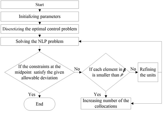
The control strategy of the AGPM is:

Step 1: Initializing parameters and setting initial number of the collocations.

Step 2: The optimal control problem at the set collocations is discretized and transformed to a NLP problem.

Step 3: Solving the NLP problem.

Step 4: Determining if the dynamic constraint, the path constraint, the state and the control constraint at the midpoint of each element satisfy the given allowable deviation $\epsilon$. If it is satisfied, the iteration stops. If not, step 5 is proceed.

Step 5: Determining if each element in the normalized midpoint residual vector $\mathbf{\beta }$ is smaller than the midpoint residual index $\rho$. If it is satisfied, step 6 is proceed. If not Step 7 is proceed.

Step 6: Increasing the number of collocations in the unit. That is to say, increasing the order of the Legendre interpolation polynomial, and then going to Step 3.

Step 7: Refining the corresponding unit to multiple units and going to Step 3.

The control block diagram is shown in Fig. 2.

Fig. 2The control block diagram of the AGPM

4.1. Simulation result

Simulation is carried out in Matlab software to verify the method.

The parameters of the real vehicle used in the simulation are shown in Table 2.

The tracked path is prescribed as the pylon course slalom test road shown in Fig. 3. A vehicle travels along the pylon course slalom test road. The vehicle should pass through the prescribed road within the minimum time.

In realistic driving process, the ideal target drivers’ trajectory should be described as a curve of order three with continuous first-order derivative:

From Eq. (31) it is easy to obtain the relationship between $y$, i.e.$f\left(x\right)$ and $x$ by substituting $t$ with $x/u$.

Fig. 3Pylon course slalom test road (● stands for stake), where s0=L=2u, s=3u, u is the longitudinal speed. B is the rotary distance, B= 2.46 m. L is the distance between the stakes

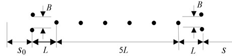
Fig. 4Fitted pylon course slalom test road

The optimization is calculated by SQP algorithm and MATLAB software in a computer which CPU is 2.8 GHz/Pentium IV, and operating system is Window XP. The minimum time for the vehicle accomplishing the pylon course slalom test road process is 14.9 seconds after 15 iterations.

Fig. 5 describes the result of the lateral distance of traveling along the pylon course slalom test road. It can be seen from the figure that the vehicle can successfully complete the pylon course slalom test road process without crossing the road boundary conditions with the speed of 90 km/h indicating good control performance of the proposed method.

Fig. 6 is the simulation result of steering torque. It can be seen from the figure that there are peak values at 140 m, 175 m, 240 m, and 280 m, indicating that the driver manipulates the car strenuously.

Fig. 5Lateral distance

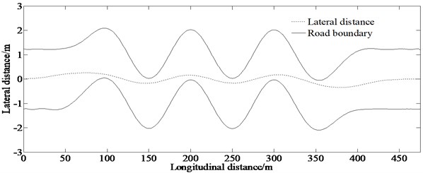
Fig. 7 is the simulation result of the traction force of front wheel. The figure indicates that the traction force of front wheel keeps growing until 1.63 kN. However, it can be seen from the curve that the curve slope keeps being small until 0 at 400 m.

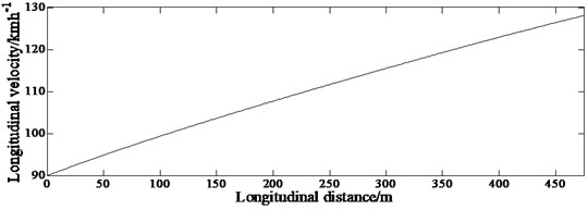
Fig. 8 is the simulation result of the longitudinal velocity. It is shown that longitudinal velocity keeps growing until 127 km/h. So, the driver should be cautious about maneuvering the car.

Fig. 6Steering torque

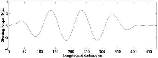
Fig. 7Traction force of front wheel

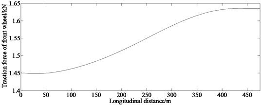
Fig. 8Longitudinal velocity

4.2. Evaluation of obstacle avoidance capability

In order to compare the obstacle avoidance capability of different vehicles in the same path trajectory conditions, another vehicle which is remarked as vehicle 2 (The vehicle referred above is remarked as vehicle 1) completes the pylon course slalom test road process without crossing the road boundary conditions with the speed of 90 km/h. And the parameters of vehicle 2 used in the simulation are shown in Table 3.

Fig. 9(a) is the simulation result of lateral displacement of the two vehicles. It can be seen that the lateral displacement of the two vehicles is almost coincident. The pattern of motion for the vehicles is that the vehicles travel along a straight line almost between the road borders. Fig. 9(b) is the simulation result of the steering torque of the two vehicles. It can also be seen from the figure that the amplitude of steering torque of vehicle 1 is larger than that of vehicle 2. The obstacle avoidance capability can be evaluated objectively by calculating the minimum time of the vehicles completing the pylon course slalom test road process. The evaluation of obstacle avoidance capability is shown in Table 4.

Fig. 9Evaluation of obstacle avoidance capability

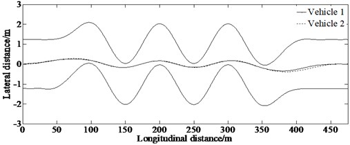
a) Lateral distance

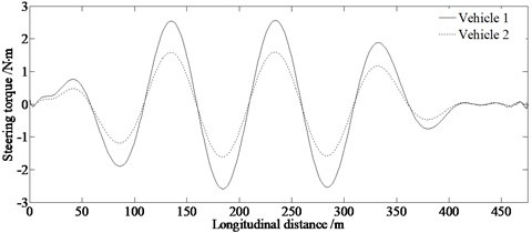
b) Steering torque

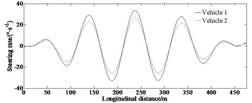
c) Steering rate

4.3. Analysis of control efficiency

In order to analyze the control efficiency of the AGPM compared with the traditional method (Direct parallel method [21] and LQR [22]), simulation with same conditions is established. The tracked trajectory is the double lane change test road.

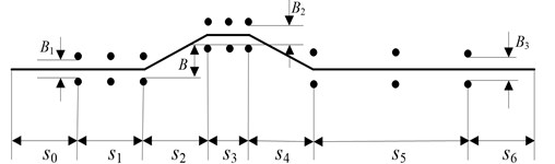
The double lane change test road is described in Fig. 10.

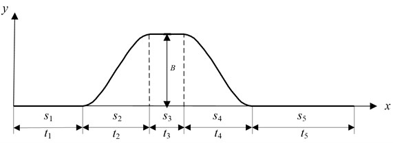
Fig. 10Double lane change test road (● stands for stake), where s0=s1=s2=s4=2u, s3=u, s5=5u, s6=3u. B is the distance of lane-change, B= 3.5 m. B1, B2 and B3 are the distances between the stakes, B1=1.1H+0.25= 2.12 m, B2=1.2H+0.25= 2.29 m, B3=1.3H+0.25= 2.46 m, where H is the width of the vehicle, H= 1.7 m

In a realistic driving process, drivers’ ideal target trajectory should be a low-level continuous smooth curve shown in Fig. 3. And also, according to ISO/TR3888-2004, the trajectory of the vehicle traveling along the pylon course slalom test road should be described as a curve of order three with continuous first-order derivative transformed with cubic splines fitting:

where:

Fig. 11Fitted double lane change test road

From Eq. (32) it is easy to obtain the relationship between $y$, i.e.$f\left(x\right)$ and $x$ by substituting $t$ with $x/u$:

where $g_0=e_0$; $g_i=e_i{u}^j\mathrm{}(j=\mathrm{1,2},3)$; $h_0=e_0^{\mathrm{\text{'}}}$; $h_i=e_i^{\mathrm{\text{'}}}{u}^j\mathrm{}(j=\mathrm{1,2},3)$.

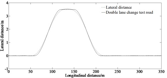
Simulation of lateral distance throughout the process of tracking the double lane change test road is shown in Fig. 12.

Fig. 12 indicates that the vehicle can track the double lane change test road well with speed of 105 km/h.

Fig. 12Lateral distance of tracking the double lane change test road

The comparison results verifying the control efficiency of the proposed method is given in Fig. 13, which including the absolute error of the lateral distance between the simulation result and the double lane change test road as well as the Steering wheel angle.

Fig. 13Evaluation of the control efficiency

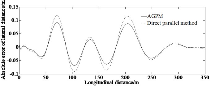
a) Absolute error of lateral distance

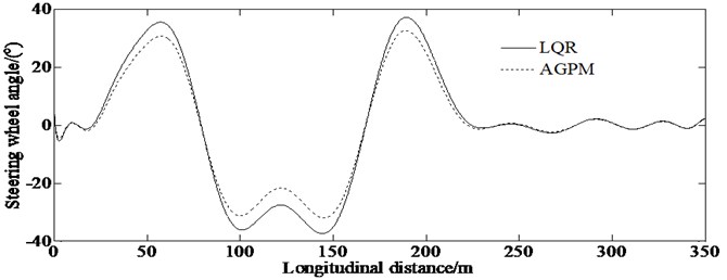
b) Steering wheel angle

From the absolute error of lateral distance curve in Fig. 13(a), it can be concluded that the maximum value of the error of lateral distance based on AGPM is less than that of the direct parallel method indicating that the AGPM is superior in calculation accuracy to the direct parallel method for solving the optimum path tracking problem of vehicle handling dynamics.

From Fig. 13(b), it can be concluded that the maximum value of the front steering angle based on the AGPM is less than that of the LQR controller. A more clear description of the evaluation of calculation accuracy is shown in Table 5.

So, it is proved that there is higher control effect for the AGPM to solve the path tracking problem comparing with other traditional methods.

4.4. Robustness verification in external disturbance environment

In this paper, a C-Class Hatchback model in Carsim is used to implement the robustness verification of the proposed algorithm.

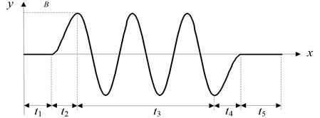
The longitudinal vehicle velocity, adhesion coefficient and maximum wind speed are set as 30 m/s, 0.8, and 50 km/h respectively. The step gust is shown in Fig. 14.

Fig. 14Step gust

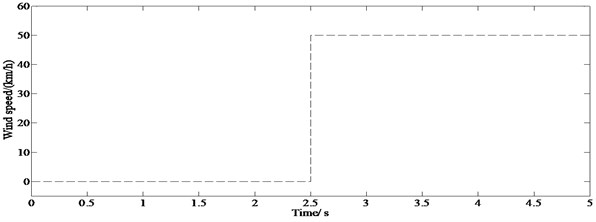
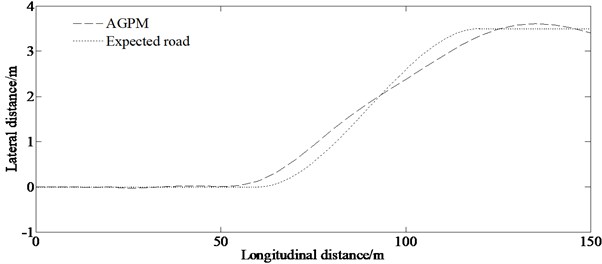
Fig. 15 shows that in the case of lateral wind, the vehicle still tracks the path well, indicating that the proposed algorithm can compensate robustness requirements in the external disturbance environment.

Fig. 15Lateral distance in external disturbance environment

4.5. Experimental result

A real vehicle test was made to verify the correctness of the proposed algorithm. The block diagram of the test system and main measurement equipment is shown in Figs. 16-18.

Fig. 16Block diagram of test system

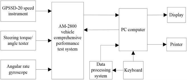
Fig. 17Measurement equipment

a) GPSSD-20 speed instrument

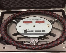
b) Steering torque/angle tester

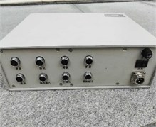
c) Comprehensive performance test system of AM-2800 vehicle

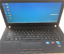
d) Lenovo computer

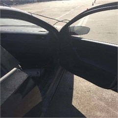
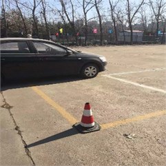
Fig. 18Real test vehicle

The test procedure in accordance with ISO/TR3888-2004 is as follows:

Step 1: Arranging stakes shown in Fig. 3.

Step 2: Placing the related equipment shown in Fig. 17.

Step 3: A water injector is installed at the center of the front axle to spray water toward the ground in order to record the real traveling trajectory.

Step 4: Repeating Step 3 process 6 times.

The test values are shown in Figs. 19(a)-19(c).

Fig. 19Comparison of simulation and test value

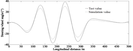
a) Steering wheel angle

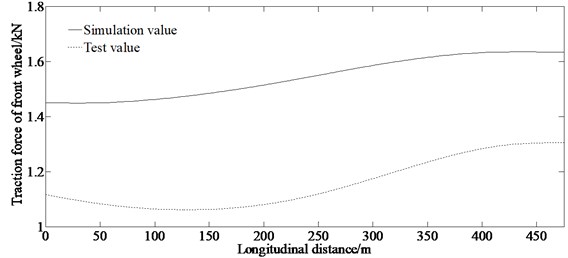
b) Traction force of front wheel

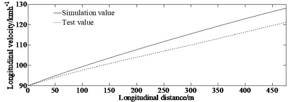
c) Longitudinal velocity

It can be seen from Fig. 19(a) that both the test value and the simulation value of the steering wheel angle have peak values at 140 m, 175 m, 240 m, and 280 m, that indicates that the driver manipulates the car strenuously. When the driver manipulates the vehicle passing the pylon course slalom test road, the driver has to increase the steering wheel angle to avoid the stakes so the test value is bigger than that of the simulation. Fig. 19(b) shows that the test value and the simulation value increase as the longitudinal distance increase, this is because the driver must tread the throttle pedal to accelerate the vehicle to track the described trajectory within the minimum time. And the figure shows that the test value is smaller than the simulation value. This is because the driver must control the gears and throttle pedal to prevent the occurrence of side slip or rolling. At the same time, there are some errors in test equipment resulting in differences between test and simulation results. As shown in Fig. 19(c), both the test value and the simulation value of the longitudinal velocity increase as the longitudinal distance increases. This is because the driver must accelerate the vehicle to track the described path within the minimum time. But the test value is smaller than the simulation value. This is reasoned by that there are psychological problems in performing a certain impact on the test results for the driver driving the vehicle at a high speed. From Fig. 19(c), it is also can be seen that the error between the simulation and the real test values increases as the longitudinal distance increases. Both the simulation and the real test values tend to two lines almost with different slopes caused by driving skill and psychological burden under the condition of vehicle tracking the described path within the minimum time. At the same time, the two lines have the same starting coordinates (0, 25), that is why the error between the simulation and the real test values occurs for the longitudinal distance.

However, the simulation and the experimental values are consistent, verifying the correctness of the proposed algorithm.

The authors declare that there is no conflict of interests regarding the publication of this paper.