Minimum-time lane changing problem of vehicle handling inverse dynamics based on adaptive mesh refinement and collocation optimization method

Liu, Yingjie; Cui, Dawei; Peng, Wen

doi:10.21595/jve.2023.23085

Journal of Vibroengineering

Browse Journal

Submit article

Published: 01 August 2023

Check for updates

Minimum-time lane changing problem of vehicle handling inverse dynamics based on adaptive mesh refinement and collocation optimization method

Yingjie Liu¹

Dawei Cui²

Wen Peng³

^{1, 2}School of Machinery and Automation, Weifang University, Weifang, 261061, Shandong, China

³State Key Laboratory of Rolling and Automation, Northeastern University, Shenyang, 110819, China

Corresponding Authors:

Yingjie Liu, Dawei Cui

Cite the article Download PDF

Downloads 131

Abstract

In order to solve the problems of multiple constraints, many different calculations of nonlinear equations which lead to major errors in the process of vehicle lane changing with minimum time, an adaptive mesh refinement and collocation optimization method is proposed. Firstly, the problem of vehicle lane changing with minimum time has been divided into nonlinear programming problems in different grids. The Lagrange interpolation polynomial was used to approximate the solution of the optimization problem in the grid, and the absolute and relative errors were resolved. Then, a mesh was determined for the unsmooth part according to the curvature of the trajectory, and the location and number of meshes were further determined according to the relationship between the maximum relative error and the allowable error. At the same time, the solution accuracy was improved by adding an adaptive calculation to the smooth interval which does not meet the tolerance error. Finally, the simulation example of comparison with the traditional optimization method was proposed. The results showed that the algorithm presented in the paper had a higher solution efficiency under the same calculation accuracy.

Minimum-time lane changing problem of vehicle handling inverse dynamics based on adaptive mesh refinement and collocation optimization method

Highlights

The method can adaptively increase the number of collocation and reduce the number of mesh.
The method can generate fewer total collocation in the solution area reducing the number of nonlinear programming equations after discretization.
The algorithm presented in the paper has a higher solution efficiency under the same calculation accuracy.

1. Introduction

The rapid development of automobile technology has brought great convenience to human travel and life, and has also driven the rapid growth of automobile ownership in recent years. At present, automobile has become one of the pillar industries of national economy in various countries. However, due to some improper operations of drivers in complex traffic scenes, more and more traffic accidents seriously threaten the safety of human life. The longitudinal and lateral movements of vehicles are not completely independent, but there is a nonlinear coupling relationship. In some cases, the longitudinal and lateral coupling nonlinear characteristics will be very significant, and will affect the accuracy of vehicle motion control and even tracking, and even cannot ensure the vehicle stability in serious cases. For example, when an intelligent vehicle encounters sudden dangerous situations such as sudden braking in front of a static obstacle in the same lane or sudden emergency braking in front of the preceding vehicle, it can learn from an experienced driver to make a lateral lane change with a large range of steering operations. And at the same time, a certain braking operation is introduced to better increase the distance from the dangerous obstacles. At this time, the motion state of the intelligent vehicle traveling with large longitudinal and lateral accelerations may exceed the boundary of the power domain corresponding to the steady state condition, leading the vehicle to enter a strong transient condition with significant nonlinear dynamic characteristics of longitudinal and lateral coupling. Under such a strong transient condition, the longitudinal component of the lateral force of the vehicle will aggravate the impact on the longitudinal speed of the vehicle. And the change of the longitudinal speed will also cause the change of the centrifugal force and the vertical load, causing interference to the lateral motion state of the vehicle. With the action range of longitudinal and lateral acceleration further approaching to the limit boundary value of the dynamic domain provided by road adhesion, the vehicle will obtain a critical instability condition. In order to ensure the control margin of the vehicle, the intelligent driving system usually limits the lateral acceleration in its trajectory plan. Therefore, under the critical instability condition, the vehicle is often accompanied by a large longitudinal acceleration, which causes a large change in the longitudinal speed, leading to a more significant nonlinear dynamics of the vehicle longitudinal and lateral coupling. As the current control strategy considers the longitudinal and lateral designs of intelligent vehicle motion separately and lacks comprehensive consideration of the above longitudinal and lateral coupling nonlinear dynamic characteristics, the vehicle motion control performance may decline significantly under strong transient, critical instability and other working conditions, which lead to vehicle instability too [1].

In the field of intelligent vehicle research, the content related to autonomous lane changing has always been one of the research hotspots in the industry. According to incomplete statistics, vehicle traffic accidents when vehicles change lanes occur every year in the quantity of about 15 %-20 %. In addition, traffic jams caused by changing lanes account for about 25 % of the total. Lane changing is a complex vehicle behavior, which not only affects the safety, efficiency and comfort of the vehicle itself, but also greatly affects the performance of the entire traffic system as a part of the traffic flow. Therefore, it is of great significance to develop a set of intelligent vehicle automatic lane changing system to meet multi-objective optimization. From the current market situation, a very mature vehicle automatic lane change system that has reached the mass production level has not yet appeared [2].

The problem of vehicle lane change motion planning has been widely studied. A brief review is presented in the following.

Naskath et al. [3] analyzed the connectivity of high-speed mobility and lane changing based on discretionary lane changing approach for V2V environment. Muhamad et al. [4] proposed a yaw rejection control for a single-trailer truck using a steerable wheel located at the middle axle of the truck. Tolga et al. [5] analyzed autonomous electric vehicles and compared their potential environmental impacts with other public transport types, carpooling, walking, cycling, and various transportation policy applications. Cao et al. [6] designed a lane change algorithm based on a look-ahead concept for the vehicle driving in front of the emergency vehicle to avoid emergency situations. Jiang et al. [7] presented a lane-level vehicle counting system which was based on V2X communications and centimeter-level positioning technologies. Yang et al. [8] presented a road environment representation method based on a dynamic occupancy grid for the lane changing assistance strategy. Vaishnavi et al. [9] developed a lane optimization model for the CAV system for solving the complexities of multilane merging areas. Amit et al. [10] proposed a microscopic traffic flow model which was intended to explain accurately the lane changing activity using Cellular Automata. Xiao et al. [11] proposed a non-lane-discipline-based car-following model for solving the problem of vehicle lane changing. Huang et al. [12] proposed a neural network-based method to predict the future status of the local vehicle using the information from V2X, and estimate the future energy consumption of each lane. Panagiotis et al. [13] proposed a methodology for modeling the likelihood of lane changing at intersections to quantify the favorability of the surrounding environment towards lane changing and simple LSTM modeling structures. Wang et al. [14] adopted a generalized dynamic model for automatic lane-changing to solve the limitations of macroscopic evaluation. H. Hamedi et al. [15] studied the vehicles’ lane change trajectories to present three novel prediction models for trajectory-grounded position. In order to investigate the characteristics of double fire sources, Guo et al. [16] performed four full-scale fire experiments in the Jiangpu road tunnel. Sharma et al. [17] proposed a novel hierarchical software architecture for the prediction of lane changing behavior on highways. Zhou et al. [18] proposed a hierarchical control strategy for the vehicle stability control. Wang et al. [19] proposed a two-stage crash causation analysis method based on the pre-crash scenarios and a crash causation derivation framework that systematically categorized and analyzed contributing factors. Wei et al. [20] proposed a prediction model based on an attention-aided encoder-decoder structure and deep neural network (DNN) to solve the problems of low prediction accuracy, difficulty in long-term prediction. Zhang et al. [21] carried out a naturalistic driving study on a highway, from which a large amount of on-road data consisting of lane-keeping and lane-changing left and right maneuvers were collected. Tajalli et al. [22] presented a methodology for optimal control of connected automated vehicles in freeway segments with a lane drop. He et al. [23] proposed a novel observation adversarial reinforcement learning approach for robust lane change decision making of autonomous vehicles. Shi, et al. [24] proposed an integrated deep learning-based two-dimension trajectory prediction model which could predict combined behaviors. Li et al. [25] proposed a lane change decision-making framework based on deep reinforcement learning to find a risk-aware driving decision strategy with the minimum expected risk for autonomous driving to ensure the driving safety.

Some of the methods provided in the above documents have large solution errors, some cannot converge to the optimal solution, and some have low accuracy. In order to solve the above problems, the relative demerits were first eliminated in discrete grids based on the hp-adaptive pseudospectral method as a direct method. Then, the mesh to be refined is determined according to the curvature of state and control variables. Finally, according to the relationship between relative and tolerance error, the number of sub grids and the number of collocations in the grid are determined, and then a solution method for vehicle lane changing with minimum time is constructed. A typical example is used to verify the effectiveness of the method. In the process of solving minimum time lane changing problem of vehicle handling inverse dynamics by a direct method, a large number of nodes need to be added to improve the accuracy of solution. So, it will lead to a dense Jacobian matrix for solving nonlinear programming problems, high order of interpolation polynomial, large amount of required calculations. Moreover, the increase of nodes will also lead to the poor convergence of the algorithm. Therefore, it is necessary to optimize the mesh and collocation. For the problem of minimum time lane changing of vehicle handling inverse dynamics, the number of sub-grid divisions is provided by using the relative error, and the location of sub-grid divisions is determined by using the density function. The adaptive mesh and refinement and collocation optimization method can approach the optimal solution by densifying the mesh and adding collocation points nearby. In areas with high smoothness, fewer collocations can be used with the strong adaptability. In the process of optimization, the mesh should not be refined for the smooth parts that do not meet the requirements of allowable error, while the collocation should be added. The method can adaptively increase the number of collocation and reduce the number of meshes, so that the total number of collocations generated in the solution area is less, reducing the number of discrete nonlinear programming equations, improving the speed of solving the optimal trajectory by the SQP method.

2. Mathematical model of vehicle lane change problem

2.1. Mathematical model of vehicle lane change problem

A nonlinear 7-DOF vehicle model shown in Fig. 1 is used to describe the vehicle lane change problem.

In the state space form, it is [26]:

1

\{\begin{array}{l} m ({\dot{v}}_{x} - r v_{y}) = (F_{x f l} + F_{x f r}) c o s δ_{f} + F_{x r l} + F_{x r r} - (F_{y f l} + F_{y f r}) s i n δ_{f}), \\ m ({\dot{v}}_{y} + r v_{x}) = (F_{x f l} + F_{x f r}) s i n δ_{f} + F_{y r l} + F_{y r r} + (F_{y f l} + F_{y f r}) c o s δ_{f}), \\ I_{z} \dot{r} = (F_{x f l} + F_{x f r}) l_{f} s i n δ_{f} + [(F_{x f r} - F_{x f l}) c o s δ_{f} + (F_{x r r} - F_{x r l})] \frac{B_{w}}{2} \\ + (F_{y f l} + F_{y f r}) l_{f} c o s δ_{f} + (F_{y f l} - F_{y f r}) \frac{B_{w}}{2} s i n δ_{f} - (F_{y r l} + F_{y r r}) l_{f} . \end{array}

The state equation can be described as:

2

\dot{x} = f [x (t), z (t)],

where $x (t)$ and $z (t)$ are the state and the input which are denoted respectively as $x (t) = {[v_{x} (t), v_{y} (t), r (t), x (t), y (t)]}^{T}$ , $z (t) = [δ (t)]^{T}$ .

The parameters and the corresponding definitions can be found in Table 1.

Fig. 1Nonlinear 7-DOF vehicle model

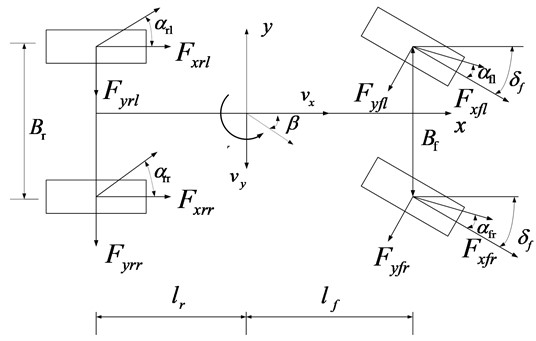
Table 1Parameter and definition

Parameter	Definition
$v_{x}$	Longitudinal speed
$v_{y}$	Lateral speed
$r$	Yaw rate of vehicle
$m$	Vehicle mass
$I_{z}$	Moment of inertia around z axis
$β$	Sideslip angle
$B_{w}$	Wheel-base of vehicle
$l_{f}$	Distances of front axle from center of gravity
$l_{r}$	Distances of rear axle from tcenter of gravity
$F_{x i j}$	Longitudinal tire force
$F_{y i j}$	Lateral tire force
$δ_{f}$	Front steering angle
where $i = f$ or $r$ , $j = l$ or $r$ , and $f l$ means the front left, $f r$ means the front right, $r l$ means the rear left, $r r$ means the rear right

2.2. Tire model

This article adopts the “Magic formula” tire model which expression is:

3

y = D s i n \{C a r c t a n [B x - E (B x - a r c t a n (B x))]\} + S,

4

Y (X) = y (x) + S_{v},

5

x = X + S_{h} .

The parameters and the corresponding definitions in Eqs. (3)-(5) can be found in Table 2.

Table 2Parameter and definition

Parameter	Definition
$B$	Stiffness factor
$C$	Shape factor
$D$	Amplitude factor
$E$	Curvature factor
$S_{h}$	Curve offset on the $x$ -axis
$S_{v}$	Curve offset on the $y$ -axis
$X$	Input variable
$Y (X)$	Output variable

2.3. Optimal control object of lane change motion planning problem

The minimum time problem of lane change motion planning can be regarded as the optimal control problem in the control theory. Therefore, the minimum time performance indicator is:

6

J = \int_{t_{0}}^{t_{f}} d t,

where:

D_{k i} (τ_{k}) = \dot{L} (τ_{k}) = \{\begin{array}{l} \frac{(1 + τ_{k}) {\dot{P}}_{N} (τ_{k}) + P_{N} (τ_{k})}{(τ_{k} - τ_{i}) [(1 + τ_{i}) {\dot{P}}_{N} (τ_{i}) + P_{N} (τ_{i})]}, i \neq k, \\ \frac{(1 + τ_{i}) {\ddot{P}}_{N} (τ_{i}) + 2 {\dot{P}}_{N} (τ_{i})}{2 [(1 + τ_{i}) {\dot{P}}_{N} (τ_{i}) + P_{N} (τ_{i})]}, i = k, \end{array}

is the initial time, $D_{k i} \in R^{N \times (N + 1)}$ is the final time.

2.4. Constrains

The initial and terminal states are described as:

7

x (t_{0}) = [v_{x} (t_{0}), 0,0, 0,0]^{T},

8

x (t_{f}) = [v_{x} (t_{f}), 0,0, x (t_{f}), y (t_{f})]^{T} .

In order to accomplish the lane change motion planning maneuver successfully, the constraints set on the longitudinal and lateral lines as well as the lateral acceleration are $0 \leq x \leq x_{b}$ , $B_{0} \leq y \leq B_{1}$ , $|a_{y}| \leq$ 3 m/s². Where $x_{b}$ is the longitudinal distance between vehicle and obstacle; $B_{0}$ and $B_{1}$ are the minimum lateral displacements required for completing lane change motion planning process and the left boundary of adjacent lane respectively [27].

When the braking maneuver is applied to decelerate the vehicle, the constraints on $F_{x f}$ , $F_{x r}$ can be rewritten in the following manner:

9

\{\begin{array}{l} F_{x f} \geq - \frac{μ m g (b + μ h_{g})}{a + b}, \\ F_{x r} = \frac{a - μ h_{g}}{b + μ h_{g}} F_{x f} . \end{array}

3. Lane changing with minimum time

3.1. Problem description

For the sake of convenience, the problem of Lane Changing with Minimum Time is transformed into a Mayer problem.

The Bolza cost function is:

10

\begin{array}{l} J = ψ (x (- 1), t_{0}, x (1), t_{f}) + \frac{t_{f} - t_{0}}{2} \int_{- 1}^{1} g (x (τ), z (τ), τ; t_{0}, t_{f}) d τ, \\ s . t . \{\begin{array}{l} \frac{d x}{d τ} = \frac{t_{f} - t_{0}}{2} f (x (τ), z (τ), τ; t_{0}, t_{f}), τ \in [- 1,1], \\ E (x (- 1), t_{0}, x (1), t_{f}) = 0, \\ C (x (τ), z (τ), τ; t_{0}, t_{f}) \leq 0, τ \in [- 1,1], \end{array} \end{array}

where $J$ is the cost function; $ψ (\cdot)$ is the Mayer type cost function; $g (\cdot)$ is the Lagrange type cost function; $f (\cdot)$ indicates the dynamic equation; $E (\cdot)$ is the boundary constraint; $C (\cdot)$ is the path constraint; $x \in R^{n}$ and $z \in R^{m}$ represent the state and control variables respectively; $t_{0}$ is the initial time; $t_{f}$ is the final time; $x (- 1)$ and $x (1)$ are the initial and final values of the state variable. Because the solution interval is [–1, 1], $t$ should be transformed as follows:

11

t = τ (t_{f} - t_{0}) / 2 + (t_{f} + t_{0}) / 2 .

In the discrete process using the HP method, the solution interval $τ \in [- 1,1]$ will be divided into $N$ grids, i.e. $S_{k} = [T_{k - 1}, T_{k}]$ , $k = 1,2, \dots, N$ , meeting $- 1 = T_{0} < T_{1} < \dots < T_{k} = 1,$ $⋃_{k = 1}^{N} S_{k} = [- 1,1]$ .

It is set that $x^{(k)} (τ)$ and $z^{(k)} (τ)$ represent the state and control variables of $S_{k}$ respectively. Then the above optimal control Bolza problem can be transformed as:

12

\begin{array}{l} J = ψ (x^{(1)} (- 1), t_{0}, x^{N} (1), t_{f}) + \frac{t_{f} - t_{0}}{2} \sum_{k = 1}^{N} \int_{T_{k - 1}}^{T_{k}} g (x^{(k)} (τ), z^{(k)} (τ), τ; t_{0}, t_{f}) d τ, \\ s . t . \{\begin{array}{l} \frac{d x^{(k)} (τ)}{d τ} = \frac{t_{f} - t_{0}}{2} f (x^{(k)} (τ), z^{(k)} (τ), τ; t_{0}, t_{f}), k = 1,2, \dots, N, \\ E (x^{(1)} (- 1), t_{0}, x^{(N)} (1), t_{f}) = 0, \\ C (x^{(k)} (τ), z^{(k)} (τ), τ; t_{0}, t_{f}) \leq 0, k = 1,2, \dots, N . \end{array} \end{array}

Because the state is continuous at the end of the grid, $x (T_{k - 1}^{+}) = x (T_{k}^{-})$ should be met at the connection point.

The pseudo-spectral method can be divided into four categories according to different orthogonal polynomials. But the discrete principle is basically the same among all polynominals. The paper takes the Radau pseudo-spectral method as an example to illustrate discrete principle of the pseudo-spectral method.

The Bolza optimal control problem is discretized on $S_{k}$ grid using LGR (Legendre-Gauss-Radau) collocation points [28]:

13

x^{(k)} (τ) \approx X^{(k)} (τ) = \sum_{j = 1}^{M_{k} + 1} X_{j}^{(k)} (τ_{i}) L_{j}^{(k)} (τ),

where:

14

L_{j}^{(k)} (τ) = \prod_{\begin{array}{l} l = 1 \\ l \neq j \end{array}}^{M_{k} + 1} \frac{τ - τ_{l}^{(k)}}{τ_{j}^{(k)} - τ_{l}^{(k)}}, τ \in [- 1, + 1],

where $L_{j}^{(k)} (τ)$ $(j = 1,2, \cdot \cdot \cdot, M_{k} + 1)$ is the Lagrange interpolating polynomials; $(τ_{1}^{(k)}, τ_{2}^{(k)}, \dots, τ_{M_{k}}^{(k)})$ are the collocation points of LGR in interval $S_{k} = [T_{k - 1}, T_{k}]$ . But $τ_{M_{k}}^{(k)} + 1 = T_{k}$ is not the collocation point. $X^{(k)}$ is the approximation of $x^{(k)}$ .

Eq. (15) can be obtained by operating difference to $τ$ :

15

\frac{d X^{k} (τ)}{d τ} = \sum_{j = 1}^{M_{k} + 1} X_{j}^{(k)} \frac{d L_{j}^{(k)} (τ)}{d τ} .

Approximation of the dynamic equation on the grid $S_{k}$ is:

16

\sum_{j = 1}^{M_{k} + 1} D_{i j}^{(k)} X_{j}^{(k)} - \frac{t_{0} - t_{f}}{2} f (X_{i}^{(k)} (τ), Z_{i}^{(k)} (τ), t (τ_{i}^{(k)}, t_{0}, t_{f})) = 0,

where:

17

D_{i j}^{(k)} = \frac{d l_{j}^{(k)} (τ_{i})}{d τ}, i = 1,2, \dots, M_{k}, j = 1,2, \dots, M_{k} + 1,

where $D_{i j}^{(k)}$ is the $M_{k} \times (M_{k} + 1)$ -dimensional LGR differential matrix on grid $S_{k}$ . Then Eq. (12) can be discretized as:

18

\begin{array}{l} J = ψ (X_{(1)}^{(1)}, t_{0}, X_{^{(M_{k} + 1)}}^{(1)}, t_{f}) + \sum_{k = 1}^{N} \sum_{j = 1}^{M_{k}} \frac{t_{k} - t_{k - 1}}{2} ω_{j}^{(k)} g (X_{j}^{(k)} (τ), Z_{j}^{(k)} (τ), t (τ_{j}^{(k)}, t_{0}, t_{f})), \\ s . t . \{\begin{array}{l} \sum_{j = 1}^{M_{k} + 1} D_{i j}^{(k)} X_{j}^{(k)} - \frac{t_{k} - t_{k - 1}}{2} f (X_{i}^{(k)} (τ), Z_{i}^{(k)} (τ), t (τ_{i}^{(k)}, t_{0}, t_{f})) = 0, \\ E (X^{(1)} (- 1), t_{0}, X^{(N)} (+ 1), t_{N}) = 0, \\ \frac{t_{k} - t_{k - 1}}{2} C (X_{i}^{(k)} (τ), Z_{i}^{(k)} (τ), t (τ_{i}^{(k)}, t_{k}, t_{k - 1})) \leq 0, \\ X_{M_{k} + 1}^{(k - 1)} = X_{1}^{(k)}, \end{array} \end{array}

where $i = 1,2, \dots, M_{k}$ ; $k = 1,2, \dots, N$ .

According to the above transformation method, the optimal control problem is transformed into a constrained nonlinear programming problem (NLP), which can be solved by the Sequential Quadratic Programming (SQP) method.

4. Adaptive optimization of mesh refinement and collocation

When the smoothness of the state and control variables is low, the solution using the global interpolation polynomial will affect its accuracy greatly. In order to improve the efficiency and accuracy of the solution, it is necessary to solve the discrete error to determine whether it is necessary or not to mesh the interpolated nodes.

4.1. Discrete error solution

It is assumed that the nonlinear programming problem shown in Eq. (10) has been already solved in interval $S_{k} = [T_{k - 1}, T_{k}]$ , $k \in [1,2, \dots, N]$ . There are $M_{k} + 1$ LGR collocation points i.e. $({\hat{τ}}_{1}^{(k)}, \dots, {\hat{τ}}_{M_{k}}^{(k)}, {\hat{τ}}_{M_{k} + 1}^{(k)})$ in $S_{k} = [T_{k - 1}, T_{k}]$ , where ${\hat{τ}}_{1}^{(k)} = τ_{1}^{(k)} = T_{k - 1}$ , ${\hat{τ}}_{M_{k} + 1}^{(k)} = T_{k}$ . It is set that the approximation of state variables in $({\hat{τ}}_{1}^{(k)}, \dots, {\hat{τ}}_{M_{k}}^{(k)}, {\hat{τ}}_{M_{k} + 1}^{(k)})$ is $(X ({\hat{τ}}_{1}^{(k)}), \dots, X ({\hat{τ}}_{M_{k}}^{(k)}), X ({\hat{τ}}_{M_{k} + 1}^{(k)}))$ . $Z ({\hat{τ}}_{1}^{(k)})$ is the approximation of control variables in $τ_{i}^{(k)}$ .

Additionally, the control in $S_{k}$ is approximated using Lagrange interpolating polynomials as:

19

Z^{(k)} (τ) = \sum_{j = 1}^{N} Z_{j}^{(k)} (τ) {\hat{L}}_{j}^{(k)} (τ),

where ${\hat{L}}_{j}^{(k)} (τ) = \prod_{l = 1, l \neq j}^{M_{k} + 1} \frac{τ - τ_{l}^{(k)}}{τ_{j}^{(k)} - τ_{l}^{(k)}}$ , $1 \leq L \leq M_{k} + 1$ , and $M_{k}$ is the number of the collocation points in interval $S_{k}$ .

Integrating the expression in Eq. (18), Eq. (20) is expressed as:

20

{\hat{X}}_{i + 1}^{(k)} ({\hat{τ}}_{j}^{(k)}) = X^{(k)} ({\hat{τ}}_{j}^{(k)}) + \frac{t_{f} - t_{0}}{2} \sum_{l = 1}^{M_{k}} I_{j l}^{(k)} f (X^{(k)} ({\hat{τ}}_{j}^{(k)}), Z^{(k)} ({\hat{τ}}_{j}^{(k)}), t ({\hat{τ}}_{j}^{(k)}, t_{0}, t_{f})),

where $I_{j i}^{(k)} (j, l = 1,2, \dots, M_{k}; k = 1,2, \dots, N)$ is a $M_{k} \times M_{k}$ LGR integral matrix of LGR collocation point in $({\hat{τ}}_{1}^{(k)}, {\hat{τ}}_{2}^{(k)} \dots, {\hat{τ}}_{M_{k}}^{(k)})$ :

21

I^{(k)} = {[D_{2}^{(k)} \dots D_{M_{k} + 1}^{(k)}]}^{- 1}, I^{(k)} D_{1}^{(k)} = 1 .

So, the relative and absolute error can be defined according to $X ({\hat{τ}}_{l}^{(k)})$ and $\hat{X} ({\hat{τ}}_{l}^{(k)})$ . The relative error $E_{i}^{(k)} ({\hat{τ}}_{l}^{(k)})$ and absolute error $e_{i}^{(k)} ({\hat{τ}}_{l}^{(k)})$ of the state variables in interval $S_{k}$ can be expressed as:

22

\{\begin{array}{l} E_{i}^{(k)} ({\hat{τ}}_{l}^{(k)}) = |{\hat{X}}_{i}^{(k)} ({\hat{τ}}_{l}^{(k)}) - X_{i}^{(k)} ({\hat{τ}}_{l}^{(k)})|, \\ e_{i}^{(k)} ({\hat{τ}}_{l}^{(k)}) = \frac{E_{i}^{(k)} ({\hat{τ}}_{l}^{(k)})}{1 + \underset{j \in [1,2, \dots, M_{k} + 1]}{m a x} |X_{i}^{(k)} ({\hat{τ}}_{j}^{(k)})|}, \end{array}

where $l = 1,2, \dots, M_{k} + 1$ , $i = 1,2, \dots, n_{x}$ . And $n_{x}$ is number of the state variable.

Then the maximum relative error can be defined as[29]:

23

e_{m a x}^{(k)} = \underset{\begin{array}{l} l \in [1,2, \dots, M_{k} + 1] \\ i \in [1,2, \dots, n_{x}] \end{array}}{m a x} e_{i}^{(k)} ({\hat{τ}}_{l}^{(k)}) .

4.2. Error range determination

Relationship between the estimated value $(\hat{y}, \hat{u})$ of LGR discrete interval and its analytical solution $(y^{*}, u^{*})$ is:

24

{‖(\hat{y} - y^{*})‖}_{\infty} + {‖\hat{u} - u^{*}‖}_{\infty} \leq \frac{c_{1} h^{q}}{N^{q - \frac{5}{2}}},

where $c_{1}$ is a constant; $N$ is number of the collocation point; $h$ is the interval width; $q$ is the minimum value of the order of consecutive derivatives solved and $N$ ; ${‖•‖}_{\infty}$ is interval norm.

4.3. Mesh refinement method

The solution result of Section 4.1 is used to determine whether the maximum relative error exceeds the tolerance error $ε$ or not. If there is a grid relative error exceeding the tolerance error $ε$ , then the grid will be divided into smaller grids or the number of collocation point can be increased within the grid. When the state and control variables in the mesh are less smooth, the solution accuracy can be improved by refining the mesh. At the same time, when the state and control variables are smooth enough, the number of collocation points in the mesh is increased. Then the solution accuracy is improved by increasing the order of the interpolation polynomial.

4.3.1. Unsmooth mesh determination

It is assumed that the optimal solution on the $m$ th interval, i.e. $S_{m}$ , has been solved using the Radau pseudo-spectral method. And it is set that the solution of the state variable in $M$ th iteration is $X^{(m)} (τ) = [X_{1}^{(m)} (τ), \dots, X_{n_{y}}^{(m)} (τ)]$ . Then continuous trajectory of the state and the control variable can be obtained by operating Lagrange interpolation on the state variable in $S_{m}$ . So, the curvature of the trajectory can be expressed as:

25

k_{i}^{m} (τ) = \frac{|x_{m_{i}}^{''} (τ)|}{{|1 + x_{m_{i}}^{'} (τ)^{2}|}^{\frac{3}{2}}}, m = 1,2, \dots, M_{k}, i = 1,2, \dots, n_{x},

where $k_{i}^{m} (τ)$ is the curvature of the $i$ th state variable in $S_{m}$ . Since each state variable has a different curvature change in $S_{m}$ , the maximum value is taken as a judgment to determine whether the trajectory is smooth or not:

26

k^{m} (τ) = \underset{i = 1,2, \dots, n_{x}}{m a x} \{k_{i}^{m} (τ)\} .

If the curvature is satisfied with:

27

k^{m} (τ) \geq \bar{k},

where $\bar{k}$ is the set curvature value, indicating that the trajectory is relatively smooth in the interval, and the interval needs to be further divided. Otherwise, the trajectory is smooth in the interval, and the accuracy of the solution can be improved by increasing the number of points.

For control variables, the same method can be used to define the changes of the control variable.

4.3.2. Mesh refinement method

4.3.2.1. Determination of sub-grids number

It is assumed that the curvature in grid $S_{m}$ in the $m$ th iteration meets Eq. (27), and it is known from the above analysis that the mesh needs to be refined. Taking equal sign for Eq. (24), then Eq. (28) can be obtained:

28

e_{m}^{(M)} = \frac{c_{1} {[h_{m}^{(M)}]}^{q}}{{[N_{m}^{(M)}]}^{q - 5 / 2}} .

In order to obtain the desired minimum relative error $ε$ in the $(M + 1)$ th iteration, Eq. (29) is obtained:

29

ε = \frac{c_{1} {[h_{m}^{(M + 1)}]}^{q}}{{[N_{m}^{(M + 1)}]}^{q - 5 / 2}} .

Since the grid $S_{m}$ has been refined, let $N_{m}^{(M + 1)} = N_{m}^{(M)}$ , that is, the interval of $S_{m}^{M}$ in the $m$ th interval and the iteration $S_{m}^{M + 1}$ in $(M + 1)$ th iteration have the same number of collocation points. Eq. (30) can be obtained by combining Eq. (28) and Eq. (29):

30

H = \frac{h_{m}^{(M + 1)}}{h_{m}^{(M)}} = {(\frac{e_{k}^{(M + 1)}}{ε})}^{1 / q},

where $H$ is the number of sub-grids to be divided at the next step. The relative error in $(M - 1)$ th iteration is:

31

ε_{k}^{(M - 1)} = \frac{c_{1} {[h_{m}^{(M - 1)}]}^{q}}{{[N_{m}^{(M - 1)}]}^{q - 5 / 2}},

$q$ can be solved by combining Eq. (28). And then the number of sub-intervals can be determined according to Eq. (30). Eq. (24) demonstrates that the number of sub-intervals newly divided is at least $H$ to ensure that the relative error in the iterative process can meet the requirements. But for a specific problem, $H$ may be larger, so this will lead to a rapid increase in the amount of calculations, so it is necessary to set upper limit of $H$ . In the study of the paper, the number of the largest subinterval of $S_{m}$ is obtained based on the ratio of relative and set error:

32

H_{m a x} = [l o g_{N} (\frac{e^{(m)}}{e})],

where $[•]$ indicates taking an integer down. Eq. (32) gives the range of the largest subinterval. Its division process is as follows. When $e^{(m)} \to ε$ , Eq. (32) may cause the value of $H_{m a x}$ to be too large, resulting in the sub-grid being redundancy. When $e^{(m)} \to ε$ , $H_{m a x}$ decreases until it is 0 gradually. So $H_{m a x}$ always provides a reasonable number of subintervals. Then $S_{m}$ will be divided into:

33

S = m i n (|H|, H_{m a x}) .

Eq. (33) gives the number of divided meshes but does not give the meshing position.

4.3.2.2. Determination of sub-grid position

In order to determine the location of the sub-grid, density function and cumulative distribution function are defined firstly. Let $f : [x, y] \to R^{+} (x, y \in R)$ be a non-negative Lebesgue integrable function, and $\int_{x}^{y} f (t) d t = 1$ , as well as $f$ be a density function. Then the integral of the density function on the defined domain is defined as the cumulative distribution function:

34

F (t) = \int_{x}^{y} f (τ) d τ .

If $L$ collocation points ${\{τ_{i}\}}_{i = 1}^{L} = 1$ ( $τ_{1} = T_{k - 1}, τ_{L} = T_{k}$ ) are inserted in interval $[T_{k - 1}, T_{k}]$ , and if position of $τ_{i}$ is determined, then the position of $τ_{i + 1}$ is:

35

F (τ_{i + 1}) - F (τ_{i}) = \frac{1}{L} .

The density function based on the curvature has a dense distribution at the position where the curvature is large, and the node distribution is sparse in a small curvature. Therefore, the cumulative distribution function can be used to determine the position of the newly added grid point. The density function can be defined by Eq. (25):

36

ρ (τ) = c_{2} k {(τ)}^{1 / 3},

where $c_{2}$ is a selected constant and meeting the following constraint:

37

\int_{- 1}^{1} ρ (τ) d τ = \int_{- 1}^{1} c_{2} k {(τ)}^{1 / 3} d τ = 1 .

Then the cumulative distribution function can be obtained:

38

F (τ) = \int_{- 1}^{τ} ρ (ζ) d ζ, τ \in [- 1,1] .

The position of the sub-grid is determined according to Eq. (33) and Eq. (34):

39

F (τ_{i}) = \frac{i - 1}{S}, 1 \leq i \leq S + 1 .

4.3.3. Distribution addition method

It is assuming that the solution in the grid $S_{m}$ does not satisfy the set error and Eq. (27). The default trajectory is smooth on interval $S_{m}$ . Collocation points should be added to increase the order of the polynomial and to reduce its solution error. It is set that $e_{m}^{(M)}$ denote an error of the $M$ th iteration on the interval $S_{m}$ , and the grid width in the $(M + 1)$ th iteration is the same as in the $M$ th iteration, i.e. $h_{k}^{M} = h_{k}^{(M + 1)}$ . Then $N_{m}^{(M + 1)}$ can be solved as:

40

N_{m}^{(M + 1)} = N_{m}^{(M)} {(\frac{e_{m}^{(M)}}{ε})}^{1 / (q - 5 / 2)},

where $N_{m}^{(M)}$ is the number of collocation points of the $M$ th iteration on grid $S_{m}$ . Since the number of collocation points is an integer, Eq. (40) should be transformed into:

41

N_{m}^{(M + 1)} = [N_{m}^{(M)} {(\frac{e_{m}^{(M)}}{ε})}^{1 / (q - 5 / 2)}] .

In order to ensure that the order of the polynomial on grid $S_{m}$ is not too high, $N_{m a x}$ is used to limit the order of the polynomial. If $N_{m}^{(M + 1)} > N_{m a x}$ , the number of collocation points on the grid is $N_{m a x}$ .

4.4. Mesh refinement and collocation process updating

The process of grid refinement and collocation point number optimization is as follows:

Step 1. Setting the initial grid and the number of collocation points in each grid.

Step 2. Resolving the nonlinear planning problem shown in Eq. (18) using the SNOPT software package.

Step 3. If the relative error resolved is less than the set relative error $ε$ , the calculation is terminated, and the result is outputted; otherwise, Step 4 is to be done.

Step 4. Determining whether the curvature of the trajectory meets the set value $k$ , if it does not meet the requirement, go to step 4.1; otherwise, go to step 4.2.

Step 4.1. Dividing the grids according to the method in Section 4.3.2 and setting the number of collocation points.

Step 4.2. Adding the number of collocation points according to the method in Section 4.3.3 or dividing the grid.

Step 5. After all the grids and collocation points have been updated, the calculation result of previous step is taken as the initial value, and then go to Step 2.

5. Numerical simulations and experimental verification

5.1. Numerical simulations

In order to verify the effectiveness of the method proposed in this paper, the simulations are made in MATLAB. They show that the vehicle parameters are according to Ref. [28].

5.1.1. Double Lane Changing Condition

In the test of driving stability of ordinary vehicles as well as in the test of tracking ability of intelligent vehicles, the double lane changing condition is a test section used frequently. However, since the track function of standard double lane changing condition is a piecewise function with poor continuity, in order to restore the true driving track under the double lane changing condition, the hyperbolic function is used to perform nonlinear fitting. And the following results are obtained:

42

Y (X) = \frac{4.05}{2} (1 + t a n (a)) - \frac{5.7}{2} (1 + t a n (b)),

43

a = \frac{2.4}{25} (X - 27.19) - 1.2,

44

b = \frac{2.4}{21.95} (X - 56.46) - 1.2,

where $X$ and $Y$ are the longitudinal and lateral positions respectively.

Fig. 2 shows the results of the lateral displacement, steering wheel angle, lateral acceleration, yaw rate and longitudinal speed under the double lane change road condition with the initial speed of 108 km/h.

From Fig. 2(a), it can be seen that the vehicle can track the double lane change road basically with the control of the proposed algorithm.

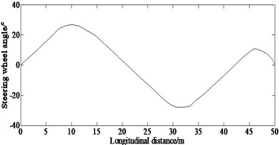
From Fig. 2(b), it can be seen that a large steering wheel angle is required to enter and exit the corners of the double lane change road. Especially, when entering the first corner and exiting the fourth corner of the double lane change road, the steering wheel angle reaches its maximum values.

From Fig. 2(c), it also can be seen that the lateral acceleration is higher at 60 m, 100 m, 430 m and 490 m; that indicates that when entering and exiting the corners of the double lane change road, the vehicle will generate the highest lateral acceleration.

From Fig. 2(d), it also can be seen that the yaw rate is higher at 60 m, 100 m, 430 m and 490 m; that indicates that when entering and exiting the corners of the double lane change road, the vehicle will generate a greater yaw rate.

From Fig. 2(e), it also can be seen that to complete the process of passing the double lane change road with minimum time, the vehicle must establish continuous acceleration.

Fig. 2Simulation results of the state variables under the double lane change condition

a) Lateral displacement

b) Steering wheel angle

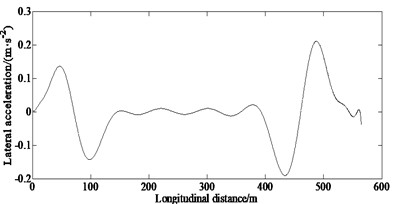
c) Lateral acceleration

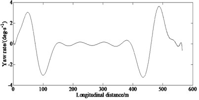
d) Yaw rate

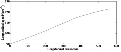
e) Longitudinal speed

5.1.2. Overtaking condition

Overtaking is a common operation mode in the process of vehicle driving.

Figs. 3(a)-(d) show the simulation results under the overtaking condition.

From Fig. 3(a), it can be seen that the vehicle can complete the processing of overtaking basically with the control of the proposed algorithm.

From Fig. 3(b), it can be seen that a large steering wheel angle is required to enter the adjacent lane from the current lane. Especially, in order to maintain stability after entering the adjacent lane, a large steering wheel angle is still required.

From Fig. 3(c), it also can be seen that a high lateral acceleration is required when entering the adjacent lane from the current lane.

From Fig. 3(d), it also can be seen that the yaw rate is greater at 15 m, 36 m; that indicates that when entering and exiting the current lane, the vehicle will generate a greater yaw rate.

Fig. 3Simulation results of state variables under overtaking condition

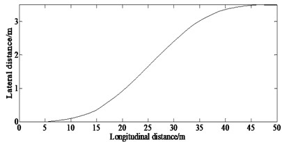
a) Lateral displacement

b) Steering wheel angle

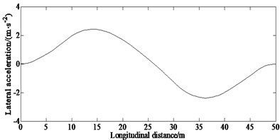
c) Lateral acceleration

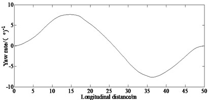
d) Yaw rate

5.2. Accuracy and efficiency verification

A comparison is made in order to verify the superiority of this method over the AMRC and GPM methods.

5.2.1. Double lane changing condition

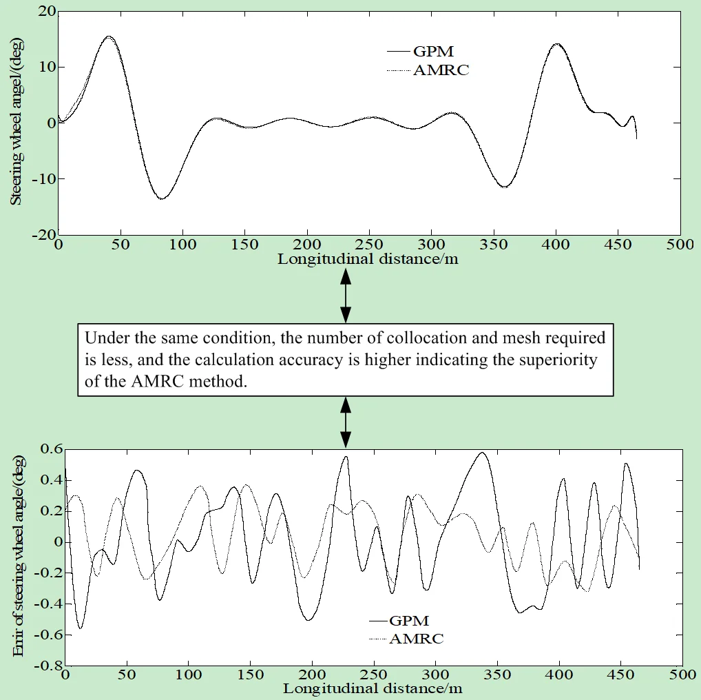
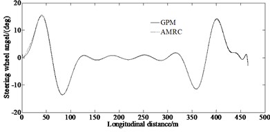
Figs. 4(a)-(c) show the simulation results of the steering wheel angle and the error of steering wheel angle obtained by the AMRC and GPM methods in the double lane changing condition.

From Fig. 4(a), it can be seen that the trend of the curves of the steering wheel angle obtained by AMRC and GPM methods is basically consistent. However, it can be seen from Fig. 4(b) that the error of steering wheel angle calculated by the AMRC is smaller than that of the GPM method. This is because the method in this paper has fewer collocation and discrete equations and sparse Jacobian matrix, so it improves the speed of solving NLP and reduces the time of optimization. Fig. 4 indicates that under the same condition, it is required a less number of collocations and meshes, so the calculation accuracy is higher. This ensures the superiority of the proposed method. And also, it can be seen from Fig. 4(c) that the mean value of estimation error of steering wheel angle of the GPM method is 0.06 deg, while the one of the AMRC method is 0.028 deg, which is smaller than that of the GPM method. This ensures the higher calculation accuracy of the proposed method.

5.2.2. Overtaking condition

In order to analyze the computational efficiency of the proposed method, the calculation accuracy is compared between the proposed method and the GPM method. The comparison results are shown in Table 3. It can be seen from the table that for the same calculation accuracy, the number of iterations and the calculation time of the hybrid method were lower than that in the direct multiple shooting method. This demonstrated that the proposed hybrid method had better solving efficiency.

Fig. 4Comparison results between AMRC and GPM under double lane changing condition

a) Steering wheel angle

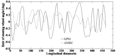
b) Error of steering wheel angle

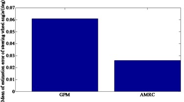
c) Mean value of estimation error of steering wheel angle

Table 3Comparison of number of iterations and calculation time of each method.

Calculation accuracy (m)	Number of iterations		Time of calculation (s)
	AMRC	GPM	AMRC	GPM
10^-2	2	4	27.36	69.47

5.3. Experimental verification

A virtual test adopting the CarSim software is conducted to verify the feasibility of the simulated results.

CarSim vehicle dynamics software can quickly build a vehicle dynamics model and driving scene of the simulated vehicle by configuring parameters, and can also conduct a real-time simulation. The vehicle dynamics model is developed in the CarSim, which is a professional vehicle system simulation software. It is adopted by many automobile manufacturers and parts suppliers in the world, and it is the standard software of the vehicle industry. CarSim adopts a system-oriented parametric modeling method. Users only need to select each vehicle component module from the model database and configure the corresponding parameters as required to complete quickly the construction of the vehicle dynamics model. CarSim offers a variety of vehicle models including sedans, pickups, and SUVs. Carsim is the vehicle state research software that uses the Vehicle Sim technology based on the vehicle dynamics and takes the simulation as the technical method. During the project development and research, the use of Carsim can greatly reduce the time spent on development, testing and planning, and allow proposing better vehicle dynamics decision-making methods. For the research projects, such simulation technology can theoretically prove the expected results, which can provide a theoretical basis for a later research and development.

In this paper, the vehicle dynamics model of the driving simulation system is quickly built in the CarSim by configuring the parameters, and the control platform and motion simulation platform are developed by using its data interface. This improves the complexity of vehicle dynamics modeling in the process of the driving simulation system development, can reduce the difficulty of vehicle dynamics modeling in the driving simulation system, and simplify the development process.

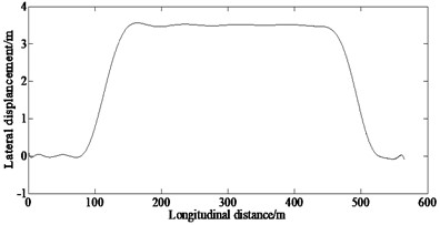
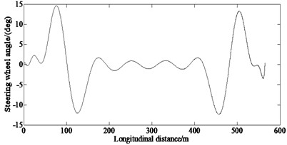
From Fig. 5, it can be seen that for the lateral displacement and the steering wheel angle as well as longitudinal speed, there are discrepancies between the simulated and the virtual test values. This is because that the model in the virtual test ignores the nonlinearity of the steering system and suspension system. However, the trend of the curves in Figs. 5(a)-(c) is enough to illustrate the correctness of the proposed method.

Fig. 5Experimental results of lateral displacement and steering wheel angle as well as longitudinal speed

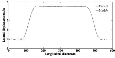
a) Lateral displacement

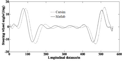
b) Steering wheel angle

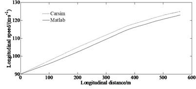
c) Longitudinal speed

6. Conclusions

To solve the problem of minimum time lane changing problem of vehicle handling inverse dynamics, this paper proposes an adaptive mesh refinement and collocation optimization method on the basis of traditional pseudo-spectral method and based on a nonlinear 7-DOF vehicle dynamics model as well as the Magic formula tire model. The simulation results show that the adaptive mesh refinement and collocation optimization method proposed in this paper can solve the problem of minimum time lane changing problem of vehicle handling inverse dynamics with high accuracy by approximating the optimal solution by densifying the mesh and adding collocation nearby. In the process of optimization solution, the method proposed in this paper can adaptively increase the number of collocations and reduce the number of meshes which can generate fewer total collocation in the solution area reducing the number of nonlinear programming equations after discretization, and improving the solving speed of the SQP method.

References

S. Cheng, L. Li, M.-M. Mei, Y.-L. Nie, and L. Zhao, “Multiple-objective adaptive cruise control system integrated with DYC,” IEEE Transactions on Vehicular Technology, Vol. 68, No. 5, pp. 4550–4559, May 2019, https://doi.org/10.1109/tvt.2019.2905858

Publisher
P. Wang, S. Gao, L. Li, B. Sun, and S. Cheng, “Obstacle avoidance path planning design for autonomous driving vehicles based on an improved artificial potential field algorithm,” Energies, Vol. 12, No. 12, p. 2342, Jun. 2019, https://doi.org/10.3390/en12122342

Publisher
J. Naskath, B. Paramasivan, Z. Mustafa, and H. Aldabbas, “Connectivity analysis of V2V communication with discretionary lane changing approach,” The Journal of Supercomputing, Vol. 78, No. 4, pp. 5526–5546, Mar. 2022, https://doi.org/10.1007/s11227-021-04086-8

Publisher
M. A. M. Yussof, N. H. Amer, Z. A. Kadir, K. Hudha, M. S. Rahmat, and M. H. Harun, “Yaw stability control of single-trailer truck using steerable wheel at middle axle: hardware-in-the-loop simulation,” International Journal of Dynamics and Control, Vol. 10, No. 6, pp. 2072–2094, Dec. 2022, https://doi.org/10.1007/s40435-022-00943-3

Publisher
T. Ercan, N. C. Onat, N. Keya, O. Tatari, N. Eluru, and M. Kucukvar, “Autonomous electric vehicles can reduce carbon emissions and air pollution in cities,” Transportation Research Part D: Transport and Environment, Vol. 112, p. 103472, Nov. 2022, https://doi.org/10.1016/j.trd.2022.103472

Publisher
W. Cao and H. Zhao, “Lane change algorithm using rule-based control method based on look-ahead concept for the scenario when emergency vehicle approaching,” Artificial Life and Robotics, Vol. 27, No. 4, pp. 818–827, Nov. 2022, https://doi.org/10.1007/s10015-022-00783-6

Publisher
J. Jiang, Y. Yang, Y. Li, R. Wang, and S. Zeng, “Lane-level vehicle counting based on V2X and centimeter-level positioning at urban intersections,” International Journal of Intelligent Transportation Systems Research, Vol. 20, No. 1, pp. 11–28, Apr. 2022, https://doi.org/10.1007/s13177-021-00271-4

Publisher
Z. Yang, Z. Gao, F. Gao, X. Wu, and L. He, “Lane changing assistance strategy based on an improved probabilistic model of dynamic occupancy grids,” Frontiers of Information Technology and Electronic Engineering, Vol. 22, No. 11, pp. 1492–1504, Nov. 2021, https://doi.org/10.1631/fitee.2000439

Publisher
T. Vaishnavi and C. Sheeba Joice, “A novel self adaptive-electric fish optimization-based multi-lane changing and merging control strategy on connected and autonomous vehicle,” Wireless Networks, Vol. 28, No. 7, pp. 3077–3099, Oct. 2022, https://doi.org/10.1007/s11276-022-03022-9

Publisher
A. K. Das and U. Chattaraj, “Cellular automata model for lane changing activity,” International Journal of Intelligent Transportation Systems Research, Vol. 20, No. 2, pp. 446–455, Aug. 2022, https://doi.org/10.1007/s13177-022-00302-8

Publisher
J. Xiao, M. Ma, S. Liang, and G. Ma, “The non-lane-discipline-based car-following model considering forward and backward vehicle information under connected environment,” Nonlinear Dynamics, Vol. 107, No. 3, pp. 2787–2801, Feb. 2022, https://doi.org/10.1007/s11071-021-06999-8

Publisher
C. Huang, L. Li, S. Fang, S. Cheng, and Z. Chen, “Energy saving performance improvement of intelligent connected PHEVs via NN-based lane change decision,” Science China Technological Sciences, Vol. 64, No. 6, pp. 1203–1211, Jun. 2021, https://doi.org/10.1007/s11431-020-1746-3

Publisher
P. Fafoutellis, J. Plymenos-Papageorgas, and E. I. Vlahogianni, “Enhancing lane change prediction at intersections with spatio-temporal adequacy information,” Journal of Big Data Analytics in Transportation, Vol. 4, No. 1, pp. 73–84, Apr. 2022, https://doi.org/10.1007/s42421-022-00055-6

Publisher
Y. Wang, X. Cao, and X. Ma, “Evaluation of automatic lane-change model based on vehicle cluster generalized dynamic system,” Automotive Innovation, Vol. 5, No. 1, pp. 91–104, Feb. 2022, https://doi.org/10.1007/s42154-021-00171-z

Publisher
H. Hamedi and R. Shad, “Context-aware similarity measurement of lane-changing trajectories,” Expert Systems with Applications, Vol. 209, p. 118289, Dec. 2022, https://doi.org/10.1016/j.eswa.2022.118289

Publisher
C. Guo, T. Zhang, Q. Guo, T. Yu, Z. Fang, and Z. Yan, “Full-scale experimental study on fire characteristics induced by double fire sources in a two-lane road tunnel,” Tunnelling and Underground Space Technology, Vol. 131, p. 104768, Jan. 2023, https://doi.org/10.1016/j.tust.2022.104768

Publisher
O. Sharma, N. C. Sahoo, and N. B. Puhan, “Highway lane-changing prediction using a hierarchical software architecture based on support vector machine and Continuous Hidden Markov model,” International Journal of Intelligent Transportation Systems Research, Vol. 20, No. 2, pp. 519–539, Aug. 2022, https://doi.org/10.1007/s13177-022-00308-2

Publisher
Y. Zhou, R. Wang, R. Ding, D. Shi, and Q. Ye, “Investigation on hierarchical control for driving stability and safety of intelligent HEV during car-following and lane-change process,” Science China Technological Sciences, Vol. 65, No. 1, pp. 53–76, Nov. 2021, https://doi.org/10.1007/s11431-021-1891-8

Publisher
X. Wang, Q. Liu, F. Guo, S.E. Fang, X. Xu, and X. Chen, “Causation analysis of crashes and near crashes using naturalistic driving data,” Accident Analysis and Prevention, Vol. 177, p. 106821, Nov. 2022, https://doi.org/10.1016/j.aap.2022.106821

Publisher
C. Wei, F. Hui, Z. Yang, S. Jia, and A. J. Khattak, “Fine-grained highway autonomous vehicle lane-changing trajectory prediction based on a heuristic attention-aided encoder-decoder model,” Transportation Research Part C: Emerging Technologies, Vol. 140, p. 103706, Jul. 2022, https://doi.org/10.1016/j.trc.2022.103706

Publisher
H. Zhang, Y. Guo, C. Wang, and R. Fu, “Stacking‐based ensemble learning method for the recognition of the preceding vehicle lane‐changing manoeuvre: A naturalistic driving study on the highway,” IET Intelligent Transport Systems, Vol. 16, No. 4, pp. 489–503, Apr. 2022, https://doi.org/10.1049/itr2.12154

Publisher
M. Tajalli, R. Niroumand, and A. Hajbabaie, “Distributed cooperative trajectory and lane changing optimization of connected automated vehicles: Freeway segments with lane drop,” Transportation Research Part C: Emerging Technologies, Vol. 143, p. 103761, Oct. 2022, https://doi.org/10.1016/j.trc.2022.103761

Publisher
X. He, H. Yang, Z. Hu, and C. Lv, “Robust lane change decision making for autonomous vehicles: an observation adversarial reinforcement learning approach,” IEEE Transactions on Intelligent Vehicles, Vol. 8, No. 1, pp. 184–193, Jan. 2023, https://doi.org/10.1109/tiv.2022.3165178

Publisher
K. Shi, Y. Wu, H. Shi, Y. Zhou, and B. Ran, “An integrated car-following and lane changing vehicle trajectory prediction algorithm based on a deep neural network,” Physica A: Statistical Mechanics and its Applications, Vol. 599, p. 127303, Aug. 2022, https://doi.org/10.1016/j.physa.2022.127303

Publisher
G. Li, Y. Yang, S. Li, X. Qu, N. Lyu, and S. E. Li, “Decision making of autonomous vehicles in lane change scenarios: Deep reinforcement learning approaches with risk awareness,” Transportation Research Part C: Emerging Technologies, Vol. 134, p. 103452, Jan. 2022, https://doi.org/10.1016/j.trc.2021.103452

Publisher
T. A. Wenzel, K. J. Burnham, M. V. Blundell, and R. A. Williams, “Dual extended Kalman filter for vehicle state and parameter estimation,” Vehicle System Dynamics, Vol. 44, No. 2, pp. 153–171, Feb. 2006, https://doi.org/10.1080/00423110500385949

Publisher
Y. Liu and Y. Liu, “Research on lane change motion planning steering input based on optimal control theory,” Mathematical Problems in Engineering, Vol. 2022, pp. 1–12, Jun. 2022, https://doi.org/10.1155/2022/8467627

Publisher
Y. Liu and J. Jiang, “Optimum path-tracking control for inverse problem of vehicle handling dynamics,” Journal of Mechanical Science and Technology, Vol. 30, No. 8, pp. 3433–3440, Aug. 2016, https://doi.org/10.1007/s12206-016-0701-9

Publisher
F. Liu, W. W. Hager, and A. V. Rao, “Adaptive mesh refinement method for optimal control using nonsmoothness detection and mesh size reduction,” Journal of the Franklin Institute, Vol. 352, No. 10, pp. 4081–4106, Oct. 2015, https://doi.org/10.1016/j.jfranklin.2015.05.028

Publisher

About this article

Received

28 November 2022

Accepted

09 May 2023

Published

01 August 2023

SUBJECTS

Vibration in transportation engineering

DOI

https://doi.org/10.21595/jve.2023.23085

Keywords

optimal control

vehicle lane changing

minimum time

mesh refinement

collocation method

Acknowledgements

This research was supported by the Science and Technology Program Foundation of Weifang under Grant 2015GX007. And also, this research was financially supported by the Open Research Fund from the State Key Laboratory of Rolling and Automation, Northeastern University, under Grant 2021RALKFKT008. The first author gratefully acknowledges the support agency.

Data Availability

The datasets generated during and/or analyzed during the current study are available from the corresponding author on reasonable request.

Author Contributions

Yingjie Liu: mathematical model and the simulation techniques. Dawei Cui: spelling and grammar checking as well as virtual validation. Wen Peng: virtual validation.

Conflict of interest

The authors declare that they have no conflict of interest.

This is an open access article distributed under the Creative Commons Attribution License, which permits unrestricted use, distribution, and reproduction in any medium, provided the original work is properly cited.

Previous article in issue Previous Next article in issue Next

Research article

2021 08 06

Optimal analysis of gear modification fitting in alternating time domain aiming at minimizing meshing-in impact of teeth-pair contact interface

Xigui Wang, Siyuan An, Yongmei Wang, Jie Tang, Jiafu Ruan

Research article

2021 05 07

Multi-objectives robust optimization based on Grey-Taguchi method for the electric vehicle frame collision

Jipeng Xie, Guolai Yang, Zhendong Zhao, Jianhua Ni

Research article

2019 12 31

Path tracking with minimum time of vehicle handling inverse dynamics based on adaptive gauss pseudospectral method

Yongsheng Liu, Yingjie Liu

Research article

2017 12 31

Adaptive mesh refinement method for optimal control based on Hermite-Legendre-Gauss-Lobatto direct transcription

Humin Lei, Tao Liu, Deng Li, Jikun Ye

Y. Liu, D. Cui, and W. Peng, “Minimum-time lane changing problem of vehicle handling inverse dynamics based on adaptive mesh refinement and collocation optimization method,” Journal of Vibroengineering, Vol. 25, No. 6, pp. 1198–1216, Aug. 2023, https://doi.org/10.21595/jve.2023.23085

Copy Extrica

Copied to clipboard!

TY  - JOUR
DO  - 10.21595/jve.2023.23085
UR  - https://doi.org/10.21595/jve.2023.23085
TI  - Minimum-time lane changing problem of vehicle handling inverse dynamics based on adaptive mesh refinement and collocation optimization method
T2  - Journal of Vibroengineering
AU  - Liu, Yingjie
AU  - Cui, Dawei
AU  - Peng, Wen
PY  - 2023
DA  - 2023/08/01
PB  - JVE International Ltd.
SP  - 1198-1216
VL  - 25
IS  - 6
SN  - 1392-8716
SN  - 2538-8460
ER  - 

Copy Ris

Copied to clipboard!

@article{Liu_2023,
	doi = {10.21595/jve.2023.23085},
	url = {https://doi.org/10.21595/jve.2023.23085},
	year = 2023,
	month = {aug},
	publisher = {{JVE} International Ltd.},
	volume = {25},
	number = {6},
	pages = {1198--1216},
	author = {Yingjie Liu and Dawei Cui and Wen Peng},
	title = {Minimum-time lane changing problem of vehicle handling inverse dynamics based on adaptive mesh refinement and collocation optimization method},
	journal = {Journal of Vibroengineering}
}

Copy Bibtex

Copied to clipboard!

[1]Y. Liu, D. Cui, and W. Peng, “Minimum-time lane changing problem of vehicle handling inverse dynamics based on adaptive mesh refinement and collocation optimization method,” Journal of Vibroengineering, vol. 25, no. 6, pp. 1198–1216, Aug. 2023, doi: 10.21595/jve.2023.23085.

Copy IEEE

Copied to clipboard!

Liu, Yingjie, Dawei Cui, and Wen Peng. “Minimum-Time Lane Changing Problem of Vehicle Handling Inverse Dynamics Based on Adaptive Mesh Refinement and Collocation Optimization Method.” Journal of Vibroengineering 25, no. 6 (August 1, 2023): 1198–1216. https://doi.org/10.21595/jve.2023.23085.

Copy Chicago

Copied to clipboard!

Minimum-time lane changing problem of vehicle handling inverse dynamics based on adaptive mesh refinement and collocation optimization method

Abstract

Highlights

1. Introduction

2. Mathematical model of vehicle lane change problem

2.1. Mathematical model of vehicle lane change problem

2.2. Tire model

2.3. Optimal control object of lane change motion planning problem

2.4. Constrains

3. Lane changing with minimum time

3.1. Problem description

4. Adaptive optimization of mesh refinement and collocation

4.1. Discrete error solution

4.2. Error range determination

4.3. Mesh refinement method

4.3.1. Unsmooth mesh determination

4.3.2. Mesh refinement method

4.3.2.1. Determination of sub-grids number

4.3.2.2. Determination of sub-grid position

4.3.3. Distribution addition method

4.4. Mesh refinement and collocation process updating

5. Numerical simulations and experimental verification

5.1. Numerical simulations

5.1.1. Double Lane Changing Condition

5.1.2. Overtaking condition

5.2. Accuracy and efficiency verification

5.2.1. Double lane changing condition

5.2.2. Overtaking condition

5.3. Experimental verification

6. Conclusions

References

About this article

Related Articles