Abstract
Obtaining vehicle status in real-time and accurately during the driving process is of great significance for active safety control of the vehicle. In response to this problem, combining a 7-DOF vehicle dynamic model and the magic formula tire model, the research designed a time-sensitive and robust double cubature Kalman filter (DCKF) observation algorithm. The DCKF algorithm addressed singular value decomposition to optimize the error covariance matrix, and connected driving state observer information of the vehicle to update the observation signal realizing the real-time estimation of the vehicle state. The DCKF algorithm is verified on the simulation platform, and compared and analyzed with the virtual test with CarSim data. The results show that the DCKF algorithm has faster response speed, higher precision of the estimation of the vehicle state, and stronger real-time performance.
Highlights
- The DCKF algorithm addresses singular value decomposition to optimize the error covariance matrix.
- The DCKF algorithm connects driving state observer information of the vehicle to update the observation signal realizing the real-time estimation of the vehicle state.
- The DCKF algorithm has faster response speed, higher precision of the estimation of the vehicle state, and stronger real-time performance.
1. Introduction
With the development of information technology, more and more information technology methods have played an important role in the automotive industry. Since the 1990s, researchers have been committed to improving the performance, safety, comfort and other performance of automobiles, and developed more and more control systems, and new driving assistance systems, such as anti-lock braking systems (ABS), traction control systems, stability control system based on lateral control and active body control system, etc.
Specifically, the onboard control system implements the corresponding control logic according to the form state of the vehicle and the corresponding road condition information. And the parameters of the state estimation are usually obtained directly from the onboard sensors. But for the vehicle, the driving conditions may be very complex. Some parameters may change with different driving conditions, and the accuracy of onboard sensors may be greatly affected by factors such as temperature, noise, etc. The production cost of the sensor must be taken into account. Many parameters that are critical to vehicle control cannot be directly estimated with reliable results through sensors. At the same time, onboard sensors also generally have certain temperature drift errors and calibration errors. The above-mentioned problems greatly limit the development of onboard control systems. At present, real-time accurate estimation of vehicle motion status has become a bottleneck problem in-vehicle control systems, driver assistance systems, and automatic driving control systems. Therefore, improving the accuracy of state estimation algorithms is a key issue in the automotive field. Not only that, accurate perception of the driving status, road information, etc., can also provide reliable information for onboard early warning and monitoring [1].
In the early state estimation algorithm research, many researchers used expensive sensors in the vehicle to obtain information about the driving state of the vehicle. For example, the optical sensing element is applied to the sensor identifying some road surface information by measuring the physical conditions such as the scattering and absorption of light by the road surface. However, the water surface, ice surface, muddy road surface, etc. will significantly affect the adhesion coefficient between the tire and the road surface, to obtain the change of the adhesion coefficient between the tire and the road surface qualitatively. Sometimes, researchers through a special onboard sensor device to study the vehicle’s movement state information and the driving road surface information. This kind of sensor has more stringent requirements for the working environment, and it is susceptible to external influences. In addition, the production cost is too high, and mass production cannot be achieved. So, this kind of sensor can only be used in special scenarios. The above various reasons make these sensors unable to be promoted in the automotive industry. Researchers are more inclined to use cheap sensors to design state estimation algorithms to estimate vehicle motion state parameters and road information [2].
For automotive safety systems, a safety strategy model that reflects vehicle and road conditions which depend on the accurate grasp of the road adhesion coefficient, driving environment information and the vehicle's motion state is a key technology that must be resolved. Among them, the real-time judgment of the road adhesion coefficient and the sideslip angle is the most difficult to implement [3].
The problem of vehicle state estimation has been widely studied. A brief review is presented in what follows.
Aiming at improving vehicle dynamics control via the anti-lock braking system (ABS) by estimating friction coefficient using video data, Sabanovic et al. [4] contributed to the development of the new efficient engineering solution that increased the performance of ABS with a rule-based control strategy. Ribeiro et al. [5] solved the tire-road friction coefficient estimation method which provided a more efficient method with robust results through the knowledge of lateral tire force. Paul et al. [6] developed a rules-based -estimation algorithm that was independent of any tire model and was validated through implementation in high-fidelity vehicle dynamics simulation. Focusing on sliding-mode techniques, followed by the development of a novel friction estimation technique, Rajendran et al. [7] presented a review of existing estimation methods that was a novel slip-based estimation method and an important tool in developing the next generation ABS systems for electric vehicles. Huang et al. [8] proposed a limited-memory adaptive extended Kalman Filter that could enhance the filter stability, improve the estimation accuracy of algorithm, and increase algorithm robustness to estimate tire-road friction coefficient. Lv et al. [9] proposed a practical estimation method for the longitudinal and lateral velocities of electric vehicles. With the proposed method the velocities could be estimated under a wide range of driving conditions accurately and reliably. To deal with vehicle sideslip angle estimation, Selmanaj et al. [10] introduced an industrially amenable kinematic-based approach that was robust to a wide range of driving scenarios and did not need tire-road friction parameters or other dynamical properties of the vehicle. Marco et al. [11] presented a multi-modal sensor fusion scheme to estimate the three-dimensional vehicle velocity and attitude angles. During both regular urban drives and collision avoidance manoeuvres, the proposed algorithm was effective. Heidfeld et al. [12] developed and validated a state observer that was able to adapt the tire model according to the current road conditions for a four-wheel-drive electric vehicle to addressing the problem of improvement of modern vehicle dynamic control systems. Reina et al. [13] developed a model-based observer that estimated automatically terrain parameters using available onboard sensors. The results of the research showed the potential of the proposed observer to estimate terrain properties during operations automatically. Wang et al. [14] presented a new method that had higher accuracy for state estimation of a vehicle system under various ISO road excitation condition to address issues associated with vehicle system state estimation using an unscented Kalman filter (UKF). Tian et al. [15] proposed an improved ant lion optimization (IALO) algorithm that had a good convergence characteristic and high stability for parameter identification of hydraulic turbine governing system. Ali et al. [16] proposed Ant Lion Optimization Algorithm (ALOA) for optimal location and sizing of DG-based renewable sources for various distribution systems. The research verified the effectiveness of ALOA compared with other algorithms. Brembeck et al. [17] discussed a vehicle state observer with a focus on the estimation of the quantity’s position, yaw angle, velocity, and yaw rate. The designed state estimators was of high-performance for future autonomous vehicles. Katriniok et al. [18] proposed an extended Kalman filter-based estimator adopting a dynamic vehicle model for determining the vehicle’s longitudinal and lateral velocity as well as the yaw rate. In the nominal and perturbed vehicle parameter case requiring filter adaptation, the proposed estimator was effective. Gao et al. [19]proposed a new methodology to address the problem of tightly coupled GNSS/INS (Global Navigation Satellite System/Inertial Navigation System) integration.
The Cubature Kalman filter (CKF) relies on the determined volume points to calculate the posterior probability density function, which is a new nonlinear Gaussian filtering method. In terms of implementation form, the CKF algorithm does not need to calculate the complicated Jacobian matrix like the EKF algorithm. At the same time, it does not need to set complex parameters like the UKF algorithm. Compared with the EFK and UKF algorithms, the CKF algorithm is more rapid in calculation, having faster convergence speed and higher convergence accuracy and having been widely used in nonlinear fields. However, when the CKF algorithm calculates the error covariance, the square root method (Cholesky) used to solve it easily leads to the loss of the positive definiteness of the error covariance matrix of the CKF filter algorithm. On the basis of retaining the good characteristics of the CKF algorithm, the Double Cubature Kalman filter (DCKF) uses singular value decomposition (SVD) to solve the error covariance matrix to improve the CKF algorithm. So when solving the problem of vehicle state estimation, the DCKF algorithm has a faster response speed and higher accuracy as well as stronger real-time performance, and the vehicle state and parameters can be better estimated.
2. Mathematical model of vehicle dynamics
2.1. Vehicle model
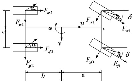
A 7-DOF nonlinear vehicle model is established as the nominal model for the design of the vehicle state estimation observer. The model includes the lateral, longitudinal and yaw motion, as shown in Fig. 1. It is assumed that the center of mass of the vehicle is the origin of the body coordinate system; there is no pitch and roll motion; the direction of the front wheel angle is the same; left and counterclockwise are the positive rotation directions; the vector in the same direction as the coordinate axis is positive.
Fig. 17-DOF vehicle model
The 7-DOF vehicle dynamics model equation is as follows.
The lateral dynamic equation is:
The longitudinal dynamic equation is:
The yaw dynamic equation is:
where, and are the longitudinal and the lateral speed; is the yaw rate, and are the longitudinal and lateral acceleration; is the moment of inertia around the -axis of the vehicle; and are the distances of front and rear axles from the center of gravity; is the vehicle mass; is the front steering angle, and are the tracks of the front and rear wheels respectively.
The wheel dynamic equation of the wheel is:
where is the moment of inertia of each wheel; is the drive torque for each wheel; is the braking torque.
2.2. Tire model
The tire is the only part of the vehicle that comes into contact with the ground. The accuracy of mathematical modeling of tires directly affects the results of vehicle dynamics simulation. This article adopts the “Magic formula” tire model which expression is:
where is the stiffness factor; is the shape factor; is the amplitude factor; is the curvature factor; is the offset of the curve on the -axis; is the offset of the curve on the -axis; is the input variable; is the output variable.
All the parameters in Eqs. (7)-(9) use the “Magic formula” tire model parameters provided in the CarSim software. in the magic tire model can be a lateral force, or it can be a normalizing moment or longitudinal force. The independent variable can represent the tire’s slip angle or longitudinal slip rate under different conditions. The coefficients , , and are determined by the vertical load and camber angle of the tire in turn.
According to the 7-DOF vehicle dynamics model, it is necessary to know the longitudinal and lateral force of the tire when predicting the state of the vehicle. The input used to calculate the tire lateral and longitudinal forces are the sideslip angle and the longitudinal slip rate of the tire respectively. The calculation formula can be derived from the vehicle model:
where is the center speed of each wheel; is the angular velocity of each wheel; is the longitudinal slip rate of each wheel; is the sideslip angle of each wheel; is the output variable; and are the track of front and rear wheels; is the rolling radius of the wheel; the subscript represents 11, 12, 21, 22; is the sideslip of the center of mass.
2.3. Nonlinear vehicle system containing noise
The vehicle driving state variable is:
The system input is:
The observation vector is:
The adhesion coefficient variable is:
The measurement output variable is:
The standard form of the state equation is:
The standard form of the measurement equation is:
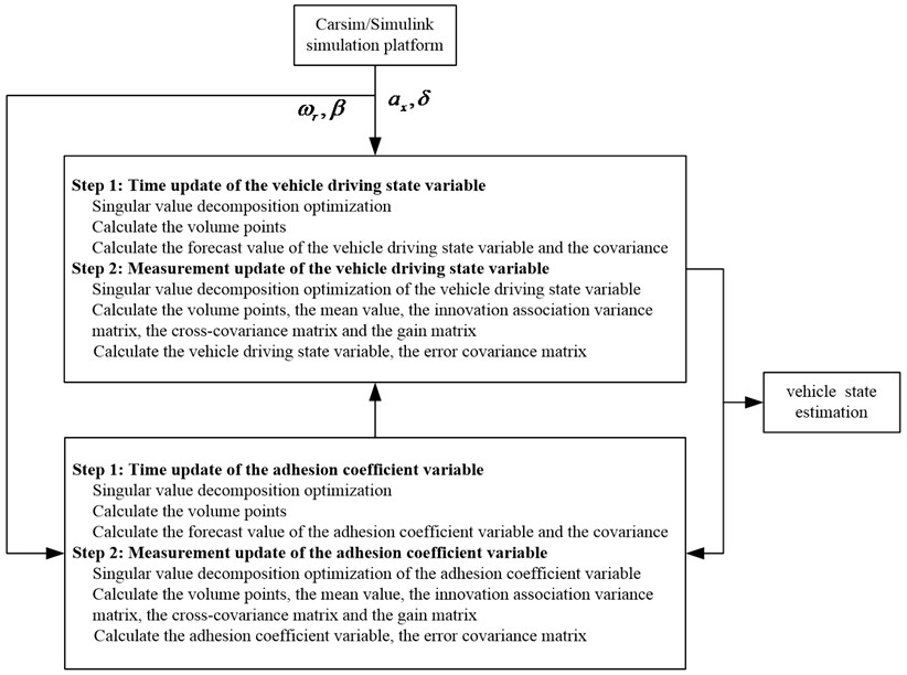
3. The DCKF observation algorithm
The DCKF algorithm cyclically links the vehicle responses to form closed-loop feedback of the information, realizing mutual correction and real-time update of the information, and improving the real-time utilization of the information. At the same time, based on the DCKF, the singular value decomposition is used to solve the error covariance matrix to improve the CKF algorithm, to realize the real-time and accurate estimation of the states.
The steps of the DCKF algorithm for vehicle state observation are as follows:
Step 1: Time updating ().
a) Singular value decomposition optimization:
where is the error covariance matrix; the column of and are the unit orthogonal eigenvector and eigenvalue of respectively; is the diagonal matrix; is the volume point; is the total number of volume points; is the state dimension; represents the th element among them. And the volume point set can be obtained:
b) Volume point :
c) Updating forecast value:
Step 2: Time updating ().
a) Singular value decomposition optimization:
where is the error covariance matrix; the column of and are the unit orthogonal eigenvector and eigenvalue of respectively; is the diagonal matrix; is the volume point; is the total number of volume points; is the state dimension; represents the th element among them. And the volume point set can be obtained:
b) Volume point :
c) Updating forecast value:
Step 3: Measurement updating ():
where is the error covariance matrix; is the volume point; is the mean value; is the innovation association variance matrix; is the cross-covariance matrix; is the gain matrix; is the adhesion coefficient variable; is the error covariance matrix.
Step 4: Measurement updating ():
where is the error covariance matrix; is the volume point; is the mean; is the innovation covariance matrix; is the cross-covariance matrix; is the gain matrix; is the vehicle driving state variables; is the Error covariance matrix.
The detailed optimization process is shown in Fig. 2.
Fig. 2DCKF algorithm flow
4. Numerical simulation and experimental verification
4.1. Numerical simulation
To verify the performance of the proposed algorithm, a certain type of vehicle is verified by a simulation test on the CarSim software. And the virtual vehicle model in Carsim is established according to the given real test vehicle. The simulation parameters in the CarSim vehicle model which are the same as our real test vehicle are shown in Table 1.
Carsim software is professional vehicle dynamics simulation software. The software has the characteristics of fast running speed, accurate calculation and easy operation. It combines people, vehicles and roads organically, and can simulate the braking and acceleration of vehicles under different road conditions. It can draw professional curves, express the trajectory of the vehicle and other difficult-to-measure quantities of the vehicle in the form of curves, and analyze various responses of the vehicle. Carsim has been widely used in the development and virtual testing of electronic control units. Carsim software is mainly used to analyze and simulate vehicle handling stability, dynamics, ride comfort and economy, etc. It can also be co-simulated with various software and hardware (such as MATLAB, lab VIEW, etc.) to provide researchers with a visual interface. It is widely used in the development process of modern automobile control system. Carsim, as one kind of vehicle simulation software specially designed for vehicle dynamics research, has many advantages over other vehicle simulation software. Automobile simulation, especially the related simulation of dynamics, plays an extremely important role in the design, improvement and upgrade of the whole vehicle, and even plays a decisive role in the design of some dynamic functions and the value enhancement of the whole vehicle. Compared with ADAMS and other software, Carsim models and designs the parameters of the entire vehicle. It does not need to define the specific physical structure of each component in the software, but only needs to define the performance of each component. Therefore, it is very convenient for application, and it can also avoid errors caused by solid modeling to a large extent. And the built model is very close to the characteristics of the real vehicle. In addition, in terms of dynamics, steady-state response, and road conditions, Carsim can realize the response of vehicle to driver input, aerodynamic input, road friction coefficient, etc. When performing vehicle dynamics simulation and testing, it can not only realize the test of vehicle handling stability, power, economy, braking and ride comfort, but also realizes real-time hardware-in-the-loop testing, and can perform co-simulation with a variety of software and hardware.
Table 1Simulation parameters
Parameter | (kg) | (kg∙m2) | (m) | (m) | (m) | (m) | (m) | (m) |
Value | 1525 | 2440 | 1.48 | 1.08 | 0.432 | 1.52 | 1.59 | 0.33 |
The vehicle parameters and simulation conditions in the test specification module of CarSim are set firstly. The vehicle travels at an initial speed of 80 km/h, and the steering wheel input steering angle is set to a sinusoidal signal input with a period of 4 s and amplitude of 60°. And also, it is assumed that the vehicle is driving on roads with road adhesion coefficients of 0.9 and 0.4.
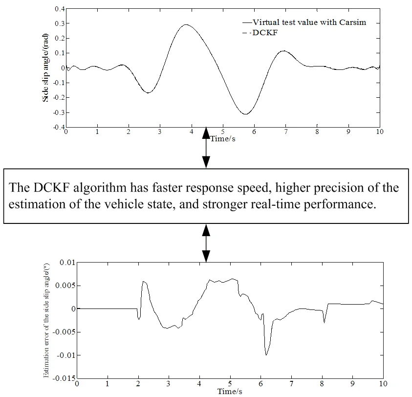
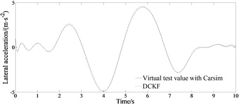
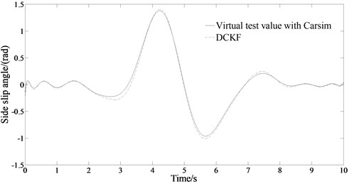
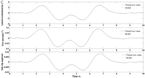
Fig. 3 shows the estimation results of the vehicle states when 0.9. It can be seen from Fig. 3 that the sine input of the steering angle works during 2 s-6 s. Fig. 3(a)-(b) shows the trend and status of the lateral acceleration and yaw rate changing according to the trend of the sinusoidal signal. It can be seen from Fig. 3(a)-(b) that the estimated changing trend of the lateral acceleration and the yaw rate is consistent with the virtual test value with CarSim indicating the good estimation performance of the algorithm. It can be seen from Fig. 3(c) that under the condition of sinusoidal signal input, the DCKF designed in the paper can accurately and effectively estimate the change of the side slipangle. And also, the estimation error is very small. The method provided in this paper considers the actual conditions of different roads, which is beneficial to solve the problems of poor real-time performance or insufficient accuracy in other sideslip angle estimation algorithm, adapting to various road conditions, and having better real-time performance and robustness.
Fig. 3Comparison results of the estimated values between the state variables and the virtual test value for a vehicle passing road with road adhesion coefficient 0.9
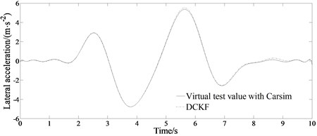
a) Estimated lateral acceleration
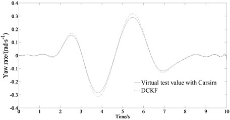
b) Estimated yaw rate
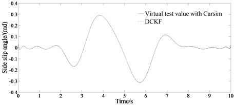
c) Estimated side slip angle
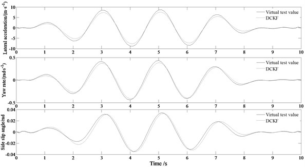
Fig. 4 shows the estimation results of the vehicle states when 0.4. Fig. 4(a)-(b) shows the trend and status of the lateral acceleration and yaw rate changing according to the trend of the sinusoidal signal. It can be seen from Fig. 4(a)-(b) that the estimated changing trend of the lateral acceleration and the yaw rate is consistent with the virtual test value with CarSim indicating the good estimation performance of the algorithm. It can be seen from Fig. 4(c) that the estimated value of the side slipangle of the center of mass at this time can also follow the change of the virtual test value with CarSim well, and has better real-time performance. In the state of sinusoidal signal input, the DCKF algorithm designed in this paper can accurately and effectively estimate the change of vehicle sideslip angle, and the estimation error is very small. Its accurate estimation can provide valid vehicle status information. Compared with the good road condition, the sideslip angle value is relatively increased, but the accuracy of the estimation is still very good, and the error is small.
Fig. 5 shows the estimation error of the slip angle under different road conditions. It can be seen from Fig. 5 that under different road conditions, the state observer designed in the paper can estimate the vehicle slip angle well with small estimation error, which can provide reliable vehicle state information for stability control. And also, under different road conditions, the estimated value obtained by the method in this paper can follow the change of the actual value in real time, which can meet the requirements of control system design. The research in this paper is of great significance for the in-depth research on the lateral stability control of vehicles in the later stage.
The performance of typical driving conditions can more faithfully reflect the handling stability of the vehicle. And also, in real traffic conditions, the double lane change road and the slalom road are the basic working conditions.
Fig. 4Comparison results of the estimated values between the state variables and the virtual test value for a vehicle passing road with road adhesion coefficient 0.4
a) Estimated lateral acceleration
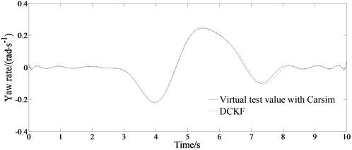
b) Estimated yaw rate
c) Estimated side slip angle
4.1.1. Double lane change road
Fig. 6 is the simulated results of the lateral acceleration, yaw rate, sideslip angle in the double lane change road condition with different speeds.
It can be seen from the Fig. 6(a) that the estimated values of the three state values are in good agreement with the virtual test values at 80 km/h. Sideslip angle and yaw rate follow slightly less at the peaks and valleys. As can be seen from the Fig. 6(b), the degree of agreement between the estimated value and the virtual test value shows that generally speaking, it still has better estimation accuracy after the vehicle speed is increased. At this time, the estimated value of the sideslip is not as good as the virtual test values, especially at the position of the peaks and valleys. This is because the change of the state value is more severe at high speed, resulting in poor follow-up of the estimated value. In addition, the lateral acceleration and yaw rate still have high estimation accuracy relative to the low-speed situation.
Fig. 5Estimation error of sideslip angle
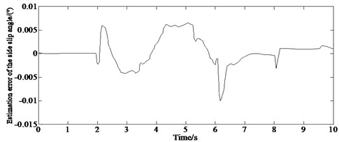
a) 0.9
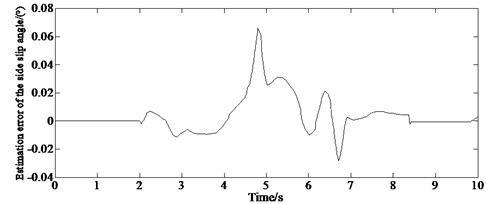
b)0.4
Fig. 6Simulated results of the lateral acceleration, yaw rate, sideslip angle in the double lane change road condition
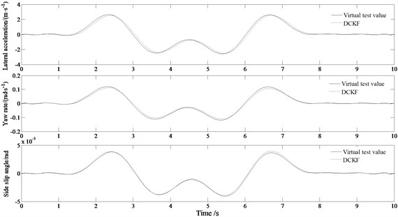
a) 80 km/h
b) 120 km/h
4.2. Slalom road
Fig. 7 is the simulated results of the lateral acceleration, yaw rate, sideslip angle in the slalom road condition with different speeds.
Fig. 7Simulated results of the lateral acceleration, yaw rate, sideslip angle in the slalom road condition
a) 80 km/h
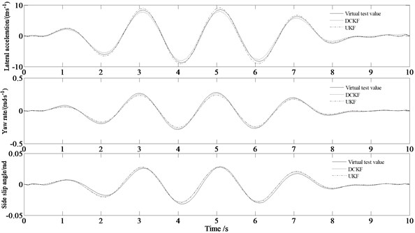
b) 120 km/h
It can be seen from the Fig. 7(a) that when the vehicle travels at a speed of 80 km/h along the slalom road, the maximum lateral acceleration has reached about 8 m/s2, and the tire has entered the nonlinear region. Generally speaking, the estimated values of the three state values are in good agreement with the virtual test values. From Fig. 7(b), it can be seen that the lateral acceleration does not change much with the increase of the vehicle speed indicating that the estimation accuracy of the lateral acceleration is not greatly affected by the vehicle speed. And also, the yaw rate of the vehicle decreases at higher speeds, which indicates that the yaw moment of the entire vehicle decreases. The estimation accuracy of the sideslip angle is roughly equivalent to that at low speeds.
The comparing results between the proposed algorithm and the UKF method (involved in reference 12) is also shown in Fig. 7(b). From Fig. 7(b) it can be seen that the accuracy and real-time performance of the DCKF estimation algorithm are better than those of the UKF estimation algorithm. This is because that the DCKF algorithm relies on the determined volume points to calculate the posterior probability density function without calculating the complex Jacobian matrix and also avoids truncation errors.
4.3. Experimental verification
In order to verify the effectiveness of the algorithm, a real vehicle test was established on a slalom test road with the speed of 65 km/h collecting the yaw rate and lateral acceleration of the vehicle with a gyroscope (Fig. 8(a)) and lateral speed with a GPSSD-20 (Fig. 8(b)) speed instrument.
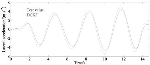
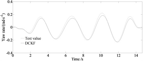
Fig. 9 is the comparison of the estimated and test values of the lateral velocity, the lateral acceleration and the yaw rate.
Fig. 8Measurement equipment: a) gyroscope, b) GPSSD-20 speed instrument
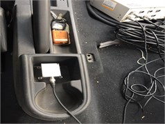
a)

b)
Fig. 9Comparison of the estimated and test values
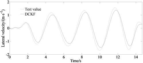
a) Test and estimated values of the lateral velocity
b) Test and estimated values of the lateral acceleration
c) Test and estimated values of the yaw rate
From the figure it can be seen that the estimated value and the experimental value are basically consistent with the curve trend. The DCKF algorithm has a better filtering effect on the yaw rate and lateral acceleration observations in the slalom road test. However, because of the adopted “Magic formula” tire model still having a certain deviation in simulating the actual tire mechanical properties and the measurement error and installation position of the sensor, there is a certain deviation in the amplitude between the estimated value and the experimental value.
5. Conclusions
We proposed a vehicle state parameter estimator to establish vehicle estimation in real-time. Finally, based on a 7-DOF vehicle model and the Magic formula tire model as well as the MATLAB simulation platform, the effectiveness of the estimation method in this paper is verified. The results show that under different road conditions, the estimated value obtained by the method in this paper can follow the change of the actual value in real-time, and can meet the requirements of the control system design. At the same, the experimental results show that under different road conditions, the estimated value obtained by the method in this paper can follow the change of the actual value in real time, and can meet the requirements of vehicle state estimation. The designed DCKF algorithm uses SVD to solve the error covariance matrix, which can update the vehicle states information in real-time. And also, the proposed DCKF algorithm is better than CKF in terms of accuracy and real-time performance, and can realize the real-time estimation of the vehicle state and parameter more accurately.
The research in this paper is of great significance to the in-depth study of the lateral stability control of electric vehicles in the later stage. The DCKF algorithm has theoretical guiding significance for the design of the estimator in the vehicle dynamic control system, and can also provide theoretical reference for the research on the testing method of the key states and parameters of the vehicle.
References
-
Y. Wang et al., “Self-learning control for coordinated collision avoidance of automated vehicles,” Proceedings of the Institution of Mechanical Engineers, Part D: Journal of Automobile Engineering, Vol. 235, No. 4, pp. 1149–1163, Mar. 2021, https://doi.org/10.1177/0954407019887884
-
S. Khaleghian, A. Emami, and S. Taheri, “A technical survey on tire-road friction estimation,” Friction, Vol. 5, No. 2, pp. 123–146, Jun. 2017, https://doi.org/10.1007/s40544-017-0151-0
-
L. Gao et al., “Multi-sensor fusion road friction coefficient estimation during steering with Lyapunov method,” Sensors, Vol. 19, No. 18, p. 3816, Sep. 2019, https://doi.org/10.3390/s19183816
-
E. Šabanovič, V. Žuraulis, O. Prentkovskis, and V. Skrickij, “Identification of road-surface type using deep neural networks for friction coefficient estimation,” Sensors, Vol. 20, No. 3, p. 612, Jan. 2020, https://doi.org/10.3390/s20030612
-
A. M. Ribeiro, A. Moutinho, A. R. Fioravanti, and E. C. de Paiva, “Estimation of tire-road friction for road vehicles: a time delay neural network approach,” Journal of the Brazilian Society of Mechanical Sciences and Engineering, Vol. 42, No. 1, pp. 1007–1025, Jan. 2020, https://doi.org/10.1007/s40430-019-2079-y
-
D. Paul, E. Velenis, F. Humbert, D. Cao, T. Dobo, and S. Hegarty, “Tyre-road friction μ-estimation based on braking force distribution,” Proceedings of the Institution of Mechanical Engineers, Part D: Journal of Automobile Engineering, Vol. 233, No. 8, pp. 2030–2047, Jul. 2019, https://doi.org/10.1177/0954407018765277
-
S. Rajendran, S. K. Spurgeon, G. Tsampardoukas, and R. Hampson, “Estimation of road frictional force and wheel slip for effective antilock braking system (ABS) control,” International Journal of Robust and Nonlinear Control, Vol. 29, No. 3, pp. 736–765, Feb. 2019, https://doi.org/10.1002/rnc.4366
-
B. Huang, X. Fu, S. Wu, and S. Huang, “Calculation algorithm of tire-road friction coefficient based on limited-memory adaptive extended kalman filter,” Mathematical Problems in Engineering, Vol. 2019, No. 5, pp. 1–14, May 2019, https://doi.org/10.1155/2019/1056269
-
J. Lv, H. He, W. Liu, Y. Chen, and F. Sun, “Vehicle velocity estimation fusion with kinematic integral and empirical correction on multi-timescales,” Energies, Vol. 12, No. 7, p. 1242, Apr. 2019, https://doi.org/10.3390/en12071242
-
D. Selmanaj, M. Corno, G. Panzani, and S. M. Savaresi, “Vehicle sideslip estimation: a kinematic based approach,” Control Engineering Practice, Vol. 67, pp. 1–12, Oct. 2017, https://doi.org/10.1016/j.conengprac.2017.06.013
-
V. Rodrigo Marco, J. Kalkkuhl, J. Raisch, W. J. Scholte, H. Nijmeijer, and T. Seel, “Multi-modal sensor fusion for highly accurate vehicle motion state estimation,” Control Engineering Practice, Vol. 100, p. 104409, Jul. 2020, https://doi.org/10.1016/j.conengprac.2020.104409
-
H. Heidfeld, M. Schünemann, and R. Kasper, “UKF-based state and tire slip estimation for a 4WD electric vehicle,” Vehicle System Dynamics, Vol. 58, No. 10, pp. 1479–1496, Oct. 2020, https://doi.org/10.1080/00423114.2019.1648836
-
G. Reina, A. Leanza, and A. Messina, “Terrain estimation via vehicle vibration measurement and cubature Kalman filtering,” Journal of Vibration and Control, Vol. 26, No. 11-12, pp. 885–898, Jun. 2020, https://doi.org/10.1177/1077546319890011
-
Z. Wang, Y. Qin, L. Gu, and M. Dong, “Vehicle system state estimation based on adaptive unscented Kalman filtering combing with road classification,” IEEE Access, Vol. 5, pp. 27786–27799, 2017, https://doi.org/10.1109/access.2017.2771204
-
T. Tian, C. Liu, Q. Guo, Y. Yuan, W. Li, and Q. Yan, “An improved ant lion optimization algorithm and its application in hydraulic turbine governing system parameter identification,” Energies, Vol. 11, No. 1, p. 95, Jan. 2018, https://doi.org/10.3390/en11010095
-
E. S. Ali, S. M. Abd Elazim, and A. Y. Abdelaziz, “Ant lion optimization algorithm for optimal location and sizing of renewable distributed generations,” Renewable Energy, Vol. 101, pp. 1311–1324, Feb. 2017, https://doi.org/10.1016/j.renene.2016.09.023
-
J. Brembeck, “Nonlinear constrained moving horizon estimation applied to vehicle position estimation,” Sensors, Vol. 19, No. 10, p. 2276, May 2019, https://doi.org/10.3390/s19102276
-
A. Katriniok and D. Abel, “Adaptive EKF-based vehicle state estimation with online assessment of local observability,” IEEE Transactions on Control Systems Technology, Vol. 24, No. 4, pp. 1368–1381, Jul. 2016, https://doi.org/10.1109/tcst.2015.2488597
-
B. Gao, G. Hu, Y. Zhong, and X. Zhu, “Cubature Kalman filter with both adaptability and robustness for tightly-coupled GNSS/INS integration,” IEEE Sensors Journal, Vol. 21, No. 13, pp. 14997–15011, Jul. 2021, https://doi.org/10.1109/jsen.2021.3073963
Cited by
About this article

