Moving horizon estimation of vehicle state and parameters

Liu, Yingjie; Cui, Dawei; Peng, Wen

doi:10.21595/jve.2022.22795

Journal of Vibroengineering

Browse Journal

Submit article

Published: 23 December 2022

Check for updates

Moving horizon estimation of vehicle state and parameters

Yingjie Liu¹

Dawei Cui²

Wen Peng³

^{1, 2}School of Machinery and Automation, Weifang University, Weifang, 261061, Shandong, China

³State Key Laboratory of Rolling and Automation, Northeastern University, Shenyang, 110819, China

Corresponding Author:

Yingjie Liu

Cite the article Download PDF

Downloads 284

Abstract

For the active safety control of the vehicle, it is extremely important to estimate the vehicle state in real-time and accurately during the driving process. A joint state and parameter estimation method based on QR decomposition and receding horizon estimation (RHE) is proposed. Firstly, by introducing the receding horizon strategy, the authors optimized the state and parameter estimation with a fixed number of variables, which can better deal with the estimation problem of time-varying parameters. Then, based on the principle of forward dynamic programming, the calculation of arrival cost is transformed into a least square equation, which is solved by QR decomposition. At the same time, an update method of arrival cost based on QR decomposition is given. In this way, the whole receding horizon estimation method is based on the optimization, and the feedback mechanism is introduced to improve the estimation accuracy and speed. The simulation results show that the accuracy of receding horizon estimation is obviously better than that of unscented Kalman filter (UKF), and the arrival cost update method based on QR decomposition is more convenient than the traditional arrival cost update method based on error covariance estimation.

Moving horizon estimation of vehicle state and parameters

Highlights

The state and parameter estimation method based on QR decomposition and receding horizon estimation (RHE) can realize the vehicle driving state estimation.
The arrival cost update method based on QR decomposition is more convenient than the traditional arrival cost update method based on error covariance estimation.
The accuracy of receding horizon estimation is obviously better than that of unscented Kalman filter (UKF).

1. Introduction

The vehicle active safety system can greatly improve the risk avoidance ability of the vehicle and effectively reduce the accident rate. The premise of its role is to obtain accurately and timely the current operation state, such as side slip angle, yaw rate and road adhesion, and then control the vehicle to maximize the driving safety by assessing the current vehicle state information. Although with the development of sensor technology, the vehicle status information can be obtained by adding corresponding sensors, it will also increase the manufacturing cost of vehicles, which is not conducive to the mass production of vehicles. The premise for the automobile active safety system to play its role is to obtain accurately and timely the current vehicle driving state information and road adhesion rate, and then to design a more rigorous control strategy to ensure the driving safety of the automobile through more complex logical relationship assessment. In recent years, the sensor technology, as an indispensable part of the control system, has developed rapidly. Although the current running state information of the vehicle can also be obtained by adding corresponding sensors, namely by adding a speedometer to obtain the speed information. However, it will also increase the corresponding production cost, which is not conducive to the mass production of the vehicle. At the same time, the estimation accuracy of some sensors, such as optical road adhesion coefficient sensor, is greatly affected by the environment and is prone to miscalculation. Based on the sensor information of the existing vehicle configuration, the method of using the corresponding algorithm to estimate the important parameters of vehicle can both reduce the production cost, and can have no constraints from operating environment. Moreover, even if the corresponding sensor is added to obtain the vehicle running state information, the results estimated by the algorithm can also provide the reference information for the control system or signalize to replace the sensor when it fails. Therefore, it has good economic benefits and engineering application value [1].

Although the existing research results have basically provided a ground for estimating the vehicle driving state and road adhesion rate, the estimation accuracy and efficiency of the algorithm may be further improved. For the vehicle running state estimation, the widely used method is based on the model that can describe the vehicle dynamic characteristics and Kalman filter or its improved algorithm. The estimation accuracy of this method is closely related to the accuracy of the dynamic model. But most results usually ignore the time-varying characteristics of the lateral stiffness in the vehicle driving state estimation model, resulting in the possibility of further improving the estimation accuracy. During the actual driving process of the vehicle, especially when the vehicle is in dangerous operating conditions such as sharp acceleration and sharp turning, the dynamic load of the wheel will change greatly due to the influence of body roll, acceleration and deceleration. And the tire cornering stiffness is more sensitive to the vertical load, which will make the tire cornering stiffness in the estimated model be greatly different from the initial value. So that the vehicle dynamics model calibrated according to the initial state may deviate greatly from the actual state, affecting the accuracy of vehicle driving state estimation. Therefore, the influence of wheel dynamic load shall be considered to improve the accuracy of the estimation model. This will make it possible to improve the total estimation accuracy. However, two methods commonly used in dealing with the estimation of pavement peak adhesion coefficient, namely, the estimation method based on single wheel dynamics model and the estimation method based on vehicle dynamics model, have some limitations. The first estimation method is usually based on a vehicle dynamics model with addition of the maximum adhesion coefficient, which can be transformed into an explicit tire model. And the maximum adhesion coefficient is estimated by using relevant algorithms such as Kalman filter algorithm. The estimation method based on single wheel dynamics model usually estimates the tire force firstly, and then estimates the adhesion coefficient by using the relationship between the existing mature tire model and tire force. The Dugoff tire model commonly used by the two methods cannot accurately describe the dynamic characteristics of the nonlinear region of the tire, so the estimation accuracy is low under the condition of high slip rate. Moreover, the estimation method based on the vehicle dynamics model has the problems of huge adjustment workload of the initial value of the model, which is unable to adapt to complex and changeable conditions and slow operation efficiency [2].

The problem of vehicle state estimation has been widely studied. A brief review is presented in what follows.

Wang et al. proposed a scheme of new Kalman filter to improve the estimation effect of noise interference in engineering practice [3]. Using an error-state extended Kalman filter, Liang et al. presented a scalable concept for vehicle state estimation [4]. The UKF algorithm introduces the idea of lossless transformation, which effectively overcomes the problems of low estimation accuracy and poor stability of EKF. The accuracy of the vehicle parameter estimation results will drop significantly when the system is strongly nonlinear [5]. Based on fusion of the machine learning model and the vehicle dynamics model, Yu et al. proposed a vehicle mass estimation method for intelligent vehicles [6]. Zhang et al. proposed a novel modified UKF state estimation methodology for the stability control of an electric vehicle [7]. To improve the safety and stability of land vehicles, Song et al. explored the estimation problem for different vehicle states [8]. Zhang et al. proposed a distributed bearing-based formation control scheme to extend the application domain for unmanned aerial vehicle swarm via global orientation estimation [9]. In order to improve the filtering accuracy of the filter algorithm, Liu et al. used an unscented Kalman filter and a genetic-particle swarm algorithm to estimate several vehicle key states [10, 11]. Yang et al. proposed the recursive least squares method to identify parameters of the battery [12]. Shereena et al. [13] proposed a novel method to deal with the simultaneous identification of road roughness. The idea of particle filter (PF) is to use a particle set to represent the probability which value is expressed using the random state particles extracted from the posterior probability. This filtering method has strong nonlinear adaptability and multi-modal processing ability. However, this method will cause the loss of sample validity and diversity in the resampling stage, resulting in the phenomenon of sample depletion. The particle swarm optimization particle filter algorithm is used to estimate the state of the vehicle, and achieve good results. However, the algorithm has the problems of large amount of calculation and great difficulty in engineering implementation [14]. Liu et al. proposed a modular integrated estimation algorithm to develop those intelligent driving systems for the preceding vehicle longitudinal and lateral states [15]. Based on the piecewise affine identification method, Sun et al. presented a novel approach to model the tire cornering characteristics [16]. Gao et al. proposed a new methodology to address the problem of tightly coupled GNSS/INS integration [17, 18]. Guo et al. proposed an avoidance method for mobile robots in dynamic environments with dynamic obstacle avoidance risk region [19]. Korayem et al. proposed a new approach in estimating the lateral tire forces and hitch-forces of a vehicle-trailer system [20]. In order to estimate the vehicle states and the tire-road peak adhesion coefficient sequentially for 4WIDEV, based on adaptive-square-root-cubature-Kalman-filter (ASRCKF) and partitioned similarity-principle (SP), Chen et al. proposed a longitudinal-lateral cooperative estimation algorithm [21].

As a model-based recursive filter, the EKF uses the first-order linearization method to extend the Kalman filter. It is a relatively mature and widely used state and parameter estimation method. Although the EKF can estimate the parameters by expanding the parameters into state variables, it is difficult to estimate the time-varying parameters due to the noise model. In addition, the EKF method cannot handle the constraint of states. The receding horizon estimation method starts from the perspective of optimal control problem, and introduces the receding horizon strategy, which realizes the estimation of state and parameters by solving the optimization problem. Therefore, receding horizon estimation can better deal with the constrained estimation problem and the joint state and parameter estimation problem. Therefore, based on the existing vehicle state parameter estimation results, this paper further improves the estimation accuracy, robustness and calculation efficiency of the algorithm, which is of great significance to improve the performance of vehicle active safety system.

2. Mathematical model of vehicle dynamics

2.1. 3-DOF vehicle model

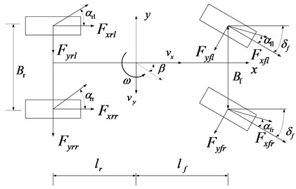
In order to facilitate the real-time estimation of the vehicle state, a vehicle dynamics model (shown in Fig. 1) is established. The model ignores the effects of suspension dynamics and wheel camber. Moreover, it is assumed that the roll angle and slope angle of the road are both zero. Among them, the $x$ -axis represents the longitudinal direction, and the driving direction of the vehicle is positive; the $y$ -axis represents the lateral direction, and the left side is positive. The meanings of the symbols in the figure are as follows: $δ_{f}$ is the front wheel angle; $v_{x}$ and $v_{y}$ are the longitudinal and lateral speeds; $β$ is the side slip angle of the center of mass; $ω$ is the yaw rate; $B_{i}$ is the wheelbase; $l_{i}$ is the distance from the axle to the center of mass; $F_{x i j}$ and $F_{y i j}$ are the longitudinal and lateral forces of the tire. $i = f, r$ represents front and rear directions; $j = l, r$ represents left and right directions. According to D’Alembert’s principle, the body dynamics equations representing longitudinal and lateral motions as well as yaw motion are as follows:

1

{\dot{v}}_{x} = v_{y} ω + a_{x},

2

{\dot{v}}_{y} = - v_{x} ω + a_{y},

3

β = a r c t a n (\frac{v_{y}}{v_{x}}),

4

\begin{array}{l} \dot{ω} F = \frac{1}{I_{z}} \{\frac{B_{f}}{2} [(F_{x f r} - F_{x f l}) c o s δ_{f} + (F_{y f l} - F_{y f r}) s i n δ_{f}] \\ + l_{f} [(F_{x f l} + F_{x f r}) s i n δ_{f} + (F_{y f l} + F_{y f r}) c o s δ_{f}] \\ + \frac{B_{f}}{2} (F_{x r r} - F_{x r l}) - l_{r} (F_{y r l} + F_{y r r})\}, \end{array}

where $a_{x}$ and $a_{y}$ are the longitudinal and lateral accelerations; $I_{z}$ is the moment of inertia of the vehicle around the $z$ -axis. Among them, the vehicle accelerations are as follows:

5

a_{x} = \frac{1}{m} [(F_{x f l} + F_{x f r}) c o s δ_{f} - (F_{y f l} + F_{y f r}) s i n δ_{f} + F_{x r l} + F_{x r r} - F_{w}],

6

a_{y} = \frac{1}{m} [(F_{x f l} + F_{x f r}) s i n δ_{f} + (F_{y f l} + F_{y f r}) c o s δ_{f} + F_{y r l} + F_{y r r}],

where $m$ is the vehicle mass; $F_{w} = ρ C_{d} A_{f} v_{x}^{2} / 2$ is the air resistance; $ρ$ is the air density; $C_{d}$ is the air resistance coefficient; $A_{f}$ is the frontal windward area of the vehicle.

The vehicle state estimation model is established based on a 3-DOF vehicle model shown in Fig. 1.

Fig. 13-DOF vehicle model

2.2. Tire dynamic model

The brush tire model is different from the complex magic formula tire model. It has few calculation parameters and can accurately describe the nonlinear relationship between tire longitudinal and lateral force, slip angle, slip rate, tire vertical load and road adhesion coefficient, etc. The combined model of longitudinal and lateral forces is defined as:

7

F = \{\begin{array}{l} C s - \frac{(C s)^{2}}{3 μ F_{z}} + \frac{(C s)^{3}}{27 (μ F_{z})^{2}}, |s| < s_{m}, \\ μ F_{z}, |s| \geq s_{m}, \end{array}

8

C = 4 a^{2} b k_{e},

9

s_{m} = \frac{3 μ F_{z}}{C},

10

s = \sqrt{s_{x}^{2} + s_{y}^{2}} .

The longitudinal and lateral forces of the tire can be expressed as:

11

F_{x} = \frac{s_{x}}{s} F, F_{y} = \frac{s_{y}}{s} F,

where $a$ is the half contact length; $b$ is the half contact width; $k_{e}$ is the tread distribution stiffness; $s$ is the total slip rate; $s_{x}$ is the longitudinal slip rate; $s_{y}$ is the lateral slip rate; $F_{z}$ is the vertical load of the tire; $μ$ is the road adhesion coefficient. Among them, the longitudinal and lateral slip rates of each tire can be expressed as:

12

s_{x i j} = \frac{R_{e} ω_{i j} - v_{i j}}{m a x (R_{e} ω_{i j}, v_{i j})}, s_{y i j} = \frac{v_{i j}}{R_{e} ω_{i j}} t a n α_{i j},

where $v_{i j}$ is the center speed of wheel; $α_{i j}$ is the slip angle of tire which calculation formula is:

13

\{\begin{array}{l} v_{f l, r} = (v_{x} \mp 0.5 B_{f} ω) c o s δ_{f} + (v_{y} + l_{f} ω) s i n δ_{f}, \\ v_{r l, r} = v_{x} \mp 0.5 B_{r} ω, \end{array}

14

\{\begin{array}{l} α_{f l, r} = δ_{f} - a r c t a n (\frac{v_{y} + l_{f} ω}{v_{x} \mp 0.5 B_{f} ω}), \\ α_{r l, r} = - a r c t a n (\frac{v_{y} - l_{f} ω}{v_{x} \mp 0.5 B_{f} ω}) . \end{array}

The formula for calculating the vertical load of each tire is:

15

\{\begin{array}{l} F_{z f l, r} = \frac{m g l_{r} - m a_{x} h_{c}}{2 (l_{f} + l_{r})} \mp \frac{a_{y}}{B_{f}} \frac{m h_{c} l_{r}}{(l_{f} + l_{r})}, \\ F_{z r l, r} = \frac{m g l_{f} + m a_{x} h_{c}}{2 (l_{f} + l_{r})} \mp \frac{a_{y}}{B_{r}} \frac{m h_{c} l_{f}}{(l_{f} + l_{r})} . \end{array}

where $h_{c}$ is the height of the center of mass of the vehicle.

2.3. Nonlinear vehicle system

The state vector of the nonlinear vehicle system is set as:

16

x = [v_{x}, r, a_{y}, β,]^{T} .

The system input is $u = [δ, a_{x}]^{T}$ , and the observation vector is:

17

y = [a_{y}, r] .

3. Receding horizon estimation based on QR decomposition

3.1. Problem description

For the continuous system shown in Eq. (18), it can be transformed into the discrete system shown in Eq. (19) by means of finite difference method, direct multiple shooting method and other methods [22]:

18

\{\begin{array}{l} \dot{x} = f (x, u), \\ y = h (x), \end{array}

19

\{\begin{array}{l} x_{k + 1} = F (x_{k}, u_{k}) + w_{k}, \\ y_{k} = H (x_{k}) + v_{k}, \end{array}

where $w_{k}$ and $v_{k}$ are the system noise sequence and measurement noise sequence respectively. Generally, it is assumed that they obey zero mean Gaussian distribution:

20

\{\begin{array}{l} w_{k} ~ N (0, Q), \\ v_{k} ~ N (0, R), \end{array}

where $Q$ and $R$ are the covariance matrices of system noise and measurement noise respectively.

The state estimation problem of system Eq. (19) can be transformed into the following optimization problem:

21

\underset{x_{0}, {\{w_{k}\}}_{k = 0}^{T - 1}}{m i n} Φ_{T} (x_{0}, \{w_{k}\}),

where:

22

Φ_{T} (x_{0}, \{w_{k}\}) = {‖x_{0} - {\hat{x}}_{0}‖}_{P_{0}^{- 1}}^{2} + \sum_{k = 0}^{T} {‖v_{k}‖}_{R^{- 1}}^{2} + \sum_{k = 0}^{T - 1} {‖w_{k}‖}_{Q^{- 1}}^{2},

where $T$ is the current time, ${\hat{x}}_{0}$ is the estimated value of the initial value of the system state; $P_{0}$ is the covariance matrix of ${\hat{x}}_{0}$ ; ${\{w_{k}\}}_{k = 0}^{T - 1}$ represents the noise sequence from time 0 to time $T - 1$ .

Eq. (21) of the optimization problem uses all the measured data, so it is called full information estimation. The amount of computation of full information estimation will rapidly increase to an unacceptable level with the growth of $T$ . Therefore, the receding horizon strategy is introduced to limit the dimension of full information estimation and form a receding horizon estimation method. The objective function of receding horizon estimation method $Φ_{T}$ becomes:

23

Φ_{T} (x_{T - N}, \{w_{k}\}) = C_{T - N} (x_{T - N}) + \sum_{k = T - N}^{T} {‖v_{k}‖}_{R^{- 1}}^{2} + \sum_{k = T - N}^{T - 1} {‖w_{k}‖}_{Q^{- 1}}^{2},

where $C_{T - N} (x_{T - N})$ is the arrival cost which is defined as follows according to the principle of forward dynamic programming:

24

\begin{array}{l} C_{T} (z) = \underset{x_{0}, {\{w_{k}\}}_{k = 0}^{T - 1}}{m i n} {‖x_{0} - {\hat{x}}_{0}‖}_{P_{0}^{- 1}}^{2} + \sum_{k = 0}^{T - N - 1} {‖v_{k}‖}_{R^{- 1}}^{2} + \sum_{k = 0}^{T - N - 1} {‖w_{k}‖}_{Q^{- 1}}^{2}, \\ s . t . x (T, x_{0}, \{w_{k}\}) = z, \end{array}

where $x (T, x_{0}, \{w_{k}\})$ indicates the value of the state at time $T$ when the initial value is $x_{0}$ and subjected to the noise sequence $\{w_{k}\}$ .

It can be seen from Eq. (24) that the arrival cost is a function with very complex expression. Therefore, the arrival cost is generally expressed by the following quadratic function:

25

Θ_{T - N} (x_{T - N}) = Φ_{T - N}^{*} + {‖x_{T - N} - {\bar{x}}_{T - N}‖}_{P_{T - N}}^{2},

where $Φ_{T - N}^{*}$ is the optimal value of optimization index at $T - N$ time; ${\bar{x}}_{T - N}$ is the state estimation at time $T - N$ ; $P_{T - N}$ is the weight matrix of the estimation error.

Due to that $Φ_{T - N}^{*}$ is a constant, the arrival cost equation presumes calculating ${\bar{x}}_{T - N}$ and $P_{T - N}$ . At present, most researches often use the Kalman filter and its error covariance matrix updating formula to calculate the arrival cost, but this method does not involve the results of receding horizon estimation, which is not conducive to the improvement of estimation accuracy and speed. From the perspective of solving optimization problems, this paper presents a calculation method of arrival cost based on QR decomposition. Since $Φ_{T - N}^{*}$ is a constant, it has no effect on the solution of the RHE problem, so it is actually important to update the arrival cost to calculate ${\bar{x}}_{T - N}$ and $P_{T - N}$ according to the estimation results. The widely used arrival cost updating algorithm is used together with the error covariance matrix updating method of EKF to calculate $P_{T - N}$ :

26

P_{T - N} = Q + G P_{T - N - 1} G^{T} - G P_{T - N - 1} C (R + C P_{T - N - 1} C^{T}) C P_{T - N - 1} G^{T},

27

\{\begin{array}{l} G = \frac{\partial F}{\partial x}, \\ C = \frac{\partial H}{\partial x} . \end{array}

3.2. Arrival cost calculation method of based on QR decomposition

At time $T + 1$ :

28

\begin{array}{l} Φ_{T + 1} (x_{T - N + 1}, \{w_{k}\}) = C_{T - N + 1} (x_{T - N + 1}) + \sum_{k = T - N + 1}^{T + 1} {‖v_{k}‖}_{R^{- 1}}^{2} + \sum_{k = T - N + 1}^{T + 1} {‖w_{k}‖}_{Q^{- 1}}^{2} \\ = C_{T - N} (x_{T - N}) + {‖v_{T - N}‖}_{R^{- 1}}^{2} + {‖w_{T - N}‖}_{Q^{- 1}}^{2} + \sum_{k = T - N + 1}^{T} {‖v_{k}‖}_{R^{- 1}}^{2} + \sum_{k = T - N + 1}^{T} {‖w_{k}‖}_{Q^{- 1}}^{2} . \end{array}

Therefore, the arrival cost is calculated in Eq. (27).

Eq. (29) can be obtained according to the principle of forward dynamic programming and Eq. (28):

29

\begin{array}{l} C_{T - N + 1} (x_{T - N + 1}) = \underset{x_{T - N}}{m i n} (C_{T - N} (x_{T - N}) + {‖v_{T - N}‖}_{R^{- 1}}^{2} + {‖w_{T - N}‖}_{Q^{- 1}}^{2}) \\ = \underset{x_{T - N}}{m i n} ({‖x_{T - N} - {\hat{x}}_{T - N}‖}_{P_{T - N}}^{2} + {‖v_{T - N}‖}_{R^{- 1}}^{2} + {‖w_{T - N}‖}_{Q^{- 1}}^{2}), \\ s . t . \{\begin{array}{l} w_{T - N} = x_{T - N + 1} - F (x_{T - N}, u_{T - N}), \\ v_{T - N} = y_{T - N} - H (x_{T - N}) . \end{array} \end{array}

For convenience expression, the weight matrices $P_{T - N}$ , $R^{- 1}$ , $Q^{- 1}$ are decomposed by Cholesky. Then Eq. (30) can be obtained as:

30

\{\begin{array}{l} P_{T - N} = {\bar{P}}_{T - N}^{T} {\bar{P}}_{T - N}, \\ R^{- 1} = ({\bar{R}}^{- 1})^{T} {\bar{R}}^{- 1}, \\ Q^{- 1} = ({\bar{Q}}^{- 1})^{T} {\bar{Q}}^{- 1} . \end{array}

Eq. (31) can be obtained according to Eq. (30):

31

C_{T - N + 1} (x_{T - N + 1}) = \underset{x_{T - N}}{m i n} {‖\begin{matrix} {\bar{P}}_{T - N} ({\bar{x}}_{T - N} - x_{T - N}) \\ {\bar{R}}^{- 1} (y_{T - N} - H (x_{T - N})) \\ {\bar{Q}}^{- 1} (x_{T - N + 1} - F (x_{T - N}, u_{T - N})) \end{matrix}‖}_{2}^{2} .

In order to obtain the analytical solution of the optimization problem shown in Eq. (31), the nonlinear functions $F$ and $H$ are linearized at the optimal estimation $x_{T - N}^{*}$ obtained by receding horizon estimation:

32

x_{T - N + 1} = F (x_{T - N}^{*}) + {\frac{\partial F}{\partial x}|}_{x_{T - N}^{*}} (x_{T - N} - x_{T - N}^{*}) = \tilde{x} + F_{x} x_{T - N},

where:

33

\{\begin{array}{l} \tilde{x} = F (x_{T - N}^{*}) - {\frac{\partial F}{\partial x}|}_{x_{T - N}^{*}} x_{T - N}^{*}, \\ F_{x} = {\frac{\partial F}{\partial x}|}_{x_{T - N}^{*}} . \end{array}

Eq. (34) can be obtained with the same method:

34

y_{T - N + 1} = H (x_{T - N}^{*}) + {\frac{\partial H}{\partial x}|}_{x_{T - N}^{*}} (x_{T - N} - x_{T - N}^{*}) = \tilde{H} + H_{x} x_{T - N},

where:

35

\{\begin{array}{l} \tilde{H} = H (x_{T - N}^{*}) - {\frac{\partial H}{\partial x}|}_{x_{T - N}^{*}} x_{T - N}^{*}, \\ H_{x} = {\frac{\partial H}{\partial x}|}_{x_{T - N}^{*}} . \end{array}

Eq. (36) can be obtained by substituting Eq. (32) and Eq. (34) into Eq. (31):

36

C_{T - N + 1} (x_{T - N + 1}) = \underset{x_{T - N}}{m i n} {‖[\begin{matrix} {\bar{P}}_{T - N} {\bar{x}}_{T - N} \\ {\bar{R}}^{- 1} (y_{T - N} - \tilde{H}) \\ - {\bar{Q}}^{- 1} \tilde{x} \end{matrix}] - [\begin{matrix} {\bar{P}}_{T - N} & 0 \\ {\bar{R}}^{- 1} H_{x} & 0 \\ {\bar{Q}}^{- 1} F_{x} & - {\bar{Q}}^{- 1} \end{matrix}] [\begin{array}{l} x_{T - N} \\ x_{T - N + 1} \end{array}]‖}_{2}^{2} .

It is set that:

37

\{\begin{array}{l} X = [\begin{matrix} x_{T - N} \\ x_{T - N + 1} \end{matrix}], \\ A = [\begin{matrix} {\bar{P}}_{T - N} & 0 \\ {\bar{R}}^{- 1} H_{x} & 0 \\ {\bar{Q}}^{- 1} F_{x} & - {\bar{Q}}^{- 1} \end{matrix}], \\ b = [\begin{matrix} {\bar{P}}_{T - N} {\bar{x}}_{T - N} \\ {\bar{R}}^{- 1} (y_{T - N} - \tilde{H}) \\ - {\bar{Q}}^{- 1} \tilde{x} \end{matrix}] . \end{array}

The arrival cost calculation problem shown in Eq. (36) is transformed into the least square problem as follows:

38

C_{T - N + 1} (x_{T - N + 1}) = \underset{x_{T - N}}{m i n} {‖b - A X‖}_{2}^{2} .

In order to solve the least square problem shown in Eq. (38), $A$ is decomposed by QR decomposition:

39

A = L [\begin{matrix} R_{1} & R_{12} \\ 0 & R_{2} \\ 0 & 0 \end{matrix}],

where $L$ is an orthogonal matrix; $R_{1}$ and $R_{2}$ are upper triangular matrices; $R_{12}$ is the lower matrix.

For convenience, Eq. (39) is simplified as:

40

L^{T} b = [\begin{array}{l} c_{1} \\ c_{2} \\ c_{3} \end{array}] .

Eq. (41) can be obtained by substituting Eqs. (39)-(40) into Eq. (38):

41

\begin{array}{l} C_{T - N + 1} (x_{T - N + 1}) = \underset{x_{T - N}}{m i n} {‖b - A X‖}_{2}^{2} \\ = \underset{x_{T - N}}{m i n} {‖b - L [\begin{matrix} R_{1} & R_{12} \\ 0 & R_{2} \\ 0 & 0 \end{matrix}] X‖}_{2}^{2} = \underset{x_{T - N}}{m i n} {‖L^{T} b - [\begin{matrix} R_{1} & R_{12} \\ 0 & R_{2} \\ 0 & 0 \end{matrix}] X‖}_{2}^{2} \\ = \underset{x_{T - N}}{m i n} {‖[\begin{array}{l} c_{1} \\ c_{2} \\ c_{3} \end{array}] - [\begin{matrix} R_{1} & R_{12} \\ 0 & R_{2} \\ 0 & 0 \end{matrix}] [\begin{array}{l} x_{T - N} \\ x_{T - N + 1} \end{array}]‖}_{2}^{2} \\ = \underset{x_{T - N}}{m i n} ({‖c_{3}‖}_{2}^{2} + {‖c_{2} - R_{2} x_{T - N + 1}‖}_{2}^{2} + {‖c_{1} - (R_{1} x_{T - N} + R_{12} x_{T - N + 1})‖}_{2}^{2}) . \end{array}

The variable in Eq. (41) is only $x_{T - N}$ , so the solution of the least squares problem is:

42

x_{T - N} = R_{1}^{- 1} (c_{1} - R_{12} x_{T - N + 1}) .

Eq. (43) can be obtained by substituting Eq. (42) into Eq. (41):

43

C_{T - N + 1} (x_{T - N + 1}) = {‖c_{3}‖}_{2}^{2} + {‖x_{T - N + 1} - R_{2}^{- 1} c_{2}‖}_{R_{2}^{T} R_{2}}^{2} .

Compared with Eq. (25), the update equation of arrival cost can be obtained:

44

\{\begin{array}{l} {\bar{x}}_{T - N + 1} = R_{2}^{- 1} c_{2}, \\ P_{T - N + 1} = R_{2}^{T} R_{2} . \end{array}

To sum up, the update calculation method of arrival cost is as follows.

Step 1: ${\bar{P}}_{T - N}$ , ${\bar{R}}^{- 1}$ and ${\bar{Q}}^{- 1}$ shall be obtained by Cholesky decomposition on the weight matrices $P_{T - N}$ , $R^{- 1}$ and $Q^{- 1}$ respectively.

Step 2: Functions $F$ and $H$ are linearized:

45

\{\begin{array}{l} x_{T - N + 1} = \bar{x} + F_{x} x_{T - N}, \\ y_{T - N} = \tilde{H} + H_{x} x_{T - N} . \end{array}

Step 3: Matrices $A$ and $b$ are constructed:

46

\{\begin{array}{l} A = [\begin{matrix} {\bar{P}}_{T - N} & 0 \\ {\bar{R}}^{- 1} H_{x} & 0 \\ {\bar{Q}}^{- 1} F_{x} & - {\bar{Q}}^{- 1} \end{matrix}], \\ b = [\begin{matrix} {\bar{P}}_{T - N} {\bar{x}}_{T - N} \\ {\bar{R}}^{- 1} (y_{T - N} - \tilde{H}) \\ - {\bar{Q}}^{- 1} \tilde{x} \end{matrix}] . \end{array}

Step 4: $Q R$ decomposition for $A$ and calculation for $L^{T} b$ is done:

47

A = L [\begin{matrix} R_{1} & R_{12} \\ 0 & R_{2} \\ 0 & 0 \end{matrix}],

48

L^{T} b = [\begin{array}{l} c_{1} \\ c_{2} \\ c_{3} \end{array}] .

Step 5: ${\bar{x}}_{T - N + 1}$ and $P_{T - N + 1}$ are calculated:

49

\{\begin{array}{l} {\bar{x}}_{T - N + 1} = R_{2}^{- 1} c_{2}, \\ P_{T - N + 1} = R_{2}^{T} R_{2} . \end{array}

Then the updating of arrival cost is completed.

3.3. Solution of rolling horizon estimation problem

It can be seen from Sections 3.1 and 3.2 that the state estimation problem of vehicle is transformed into a fixed dimension optimization problem. However, it needs to sample the system state and input. Therefore, for the continuous system of vehicle, it is necessary to choose an appropriate method to complete the discretization of the system equation. Considering the strong nonlinearity and constant sampling rate of the system, the direct multiple shooting method with constant discrete node spacing and high accuracy is selected. This method discretizes the state and control variables on discrete nodes with equal spacing. It is assumed that the control variable between adjacent nodes is constant. And the constraint of equal state variables at nodes is added to realize the discretization of continuous system. Finally, the state estimation problem is transformed into a nonlinear programming problem shown in Eq. (45):

50

\begin{array}{l} \underset{x_{T - N}, {\{w_{k}\}}_{k = T - N}^{T - 1}}{m i n} ({‖x_{T - N} - {\hat{x}}_{T - N}‖}_{P_{T - N}}^{2} + \sum_{k = T - N}^{T} {‖v_{k}‖}_{R^{- 1}}^{2} + \sum_{k = T - N}^{T - 1} {‖w_{k}‖}_{Q^{- 1}}^{2}), \\ s . t . \{\begin{array}{l} x_{k + 1} = F (x_{k}, u_{k}) + w_{k}, \\ y_{k} = H （x_{k}） + v_{k} . \end{array} \end{array}

In this paper, a more mature sequential quadratic programming method is used to solve the nonlinear programming problem in Eq. (50).

Step 1: Initialization. $P_{0}$ , $R^{- 1}$ , $Q^{- 1}$ and the initial state estimation ${\bar{x}}_{0}$ as well as the window length N of the receding horizon are set.

Step 2: When $k < N$ , the state estimation value ${\bar{x}}_{k}$ and covariance matrix $P_{k}$ are calculated using EKF updating formula.

Step 3: When $k \geq N$ , the sequential quadratic programming method is used to solve the nonlinear programming problem Eq. (50).

Step 4: ${\bar{x}}_{T - N}$ and $P_{T - N}$ are calculated using the arrival cost update strategy as described in Section 3.2.

Step 5: The measurement $y_{k + 1}$ at time $k + 1$ is done to construct a new measurement data set $[y_{k - N + 2}, \dots, y_{k}, y_{k + 1}]$ , then return to step 3.

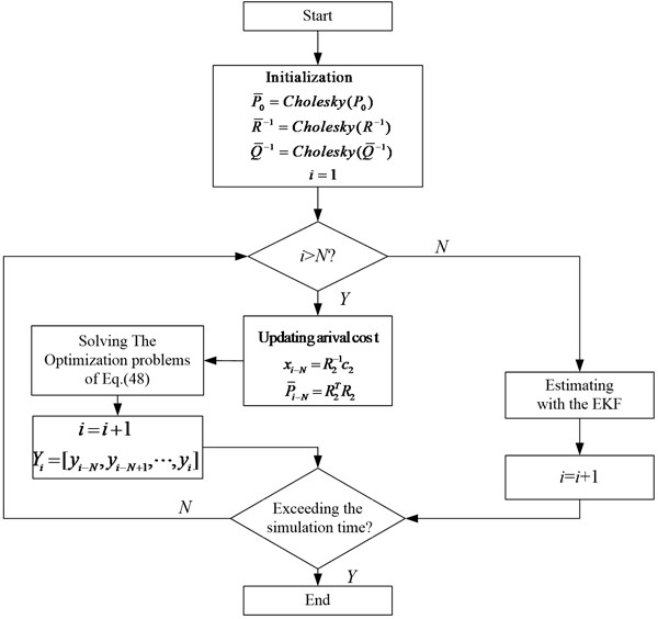
The flow of the RHE-QR algorithm is shown in Fig. 2.

Proof. The minimum sequence $Φ_{k}^{*}$ obtained by the arrival cost updating algorithm is a non-decreasing sequence. It indicates that the arrival cost value grows over time.

It is set that $x_{T - N + 1} = {\bar{x}}_{T - N + 1}$ , then Eqs. (51)-(52) can be obtained according to Eq. (41):

51

Δ k = Φ_{k}^{*} - Φ_{k + 1}^{*} = - {‖c_{3}‖}_{2}^{3} \leq 0,

52

Φ_{k + 1}^{*} \geq Φ_{k}^{*} .

Fig. 2Flow chart of RHE-QR algorithm

The arrival cost given by the arrival cost updating algorithm is bounded, indicating that the influence of historical data on the estimation results is limited and will not increase indefinitely. That is, for any vector $v$ , there is:

53

{‖v‖}_{P_{L + 1}^{- 1}}^{2} \leq λ_{m a x} {‖v‖}_{2}^{2},

where $λ_{m a x}$ is the largest eigenvalue of the matrix $Q^{- 1}$ .

Eq. (54) can be obtained according to Eq. (37):

54

A^{T} A = {[\begin{matrix} {\bar{P}}_{T - N} & 0 \\ {\bar{R}}^{- 1} H_{x} & 0 \\ {\bar{Q}}^{- 1} F_{x} & - {\bar{Q}}^{- 1} \end{matrix}]}^{T} [\begin{matrix} {\bar{P}}_{T - N} & 0 \\ {\bar{R}}^{- 1} H_{x} & 0 \\ {\bar{Q}}^{- 1} F_{x} & - {\bar{Q}}^{- 1} \end{matrix}]

Eq. (55) can be obtained according to Eq. (39):

55

A^{T} A = {[\begin{matrix} F_{1} & F_{12} \\ 0 & F_{2} \\ 0 & 0 \end{matrix}]}^{T} [\begin{matrix} F_{1} & F_{12} \\ 0 & F_{2} \\ 0 & 0 \end{matrix}] .

Eq. (56) can be obtained by comparing the elements in the second row and second column of the right matrix of Eq. (54) and Eq. (55):

56

F_{12}^{T} F_{12} + F_{22}^{T} F_{22} = ({\bar{Q}}^{- 1})^{T} {\bar{Q}}^{- 1} = Q^{- 1} .

According to Eq. (49) and Eq. (56), for any vector $v$ , it will be:

57

{‖v‖}_{P_{T - N + 1}^{- 1}}^{2} \leq {‖v‖}_{Q^{- 1}}^{2} \leq λ_{m a x} {‖v‖}_{2}^{2} .

The arrival cost update algorithm can guarantee the stability of MHE.

According to Eq. (20), the arrival cost algorithm has the following properties:

58

C_{k} (x_{k}) = \underset{x_{k - 1}}{m i n} C_{k - 1} (x_{k - 1}) + {‖v_{k - 1}‖}_{R^{- 1}}^{2} + {‖w_{k - 1}‖}_{Q^{- 1}}^{2} .

Eq. (59) can be obtained by repeated application of Eq. (58) availably:

59

C_{L} (x_{L}) = \underset{x_{L - 1}, w_{; - N}, \dots, w_{; - 1}}{m i n} C_{L - N} (x_{L - N}) + \sum_{k = L - N}^{L - 1} ({‖v_{k}‖}_{R^{- 1}}^{2} + {‖w_{k}‖}_{Q^{- 1}}^{2}) .

Eq. (59) indicates that the arrival cost updating algorithm satisfies the condition $C_{2}$ from [23]:

60

C_{L} (x_{L}) \leq \underset{x_{L - 1}, w_{; - N}, \dots, w_{; - 1}}{m i n} C_{L - N} (x_{L - N}) + \sum_{k = L - N}^{L - 1} ({‖v_{k}‖}_{R^{- 1}}^{2} + {‖w_{k}‖}_{Q^{- 1}}^{2}) .

The arrival cost algorithm can guarantee the stability of MHE.

4. Numerical simulation and experimental verification

4.1. Numerical simulation

To verify the performance of the proposed algorithm, a certain type of vehicle is verified by a simulation test in the ADAMS software. Considering the difference between the test vehicle and the vehicle model parameters in the ADAMS software, the specific parameters of the vehicle model in ADAMS (wheelbase, wheelbase, vehicle mass, wheel radius, etc.) are adjusted to be consistent with the test vehicle. The simulation parameters are shown in Table 1.

Table 1Simulation parameters

Parameter	Value
$m$ (kg)	1515
$I_{z}$ (kg∙m²)	2430
$a$ (m)	1.39
$b$ (m)	1.08
$h$ (m)	0.45

ADAMS software uses interactive graphic environment, parts library, constraint library and force library to create a fully parameterized geometric model of mechanical system. Its solver adopts the Lagrange equation method in the multi-rigid-body system dynamics theory to establish a system dynamics equation, carry out static, kinematic and dynamic analysis of virtual mechanical system, and output displacement, velocity, acceleration and reaction force curves. The simulation of ADAMS software can be used to predict the performance of mechanical system, motion range, collision detection, peak load and calculate the input load of a finite element.

On the one hand, ADAMS is an application software for virtual prototype analysis. Users can use the software to create easily statics, kinematics and dynamic analysis on virtual mechanical systems. On the other hand, it is a virtual prototype analysis and development tool. Its open program structure and various interfaces can become a secondary development tool platform for users in special industries to conduct special types of virtual prototype analysis.

4.1.1. Chassis model

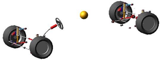
Chassis connects other systems of the whole vehicle, ignoring the specific structure of the power system and the body. The transmission system and the braking system which are simplified as rigid bodies are located on the chassis. And the center of mass is also located on the chassis. In the paper, a spherical mass block represents the concentrated mass. The size and position of the spherical mass block are not important. As long as being a part of the steering system, suspension and other components are connected to the chassis. The mass and moment of inertia of the whole vehicle can be modified by adjusting the properties of the sphere. At the same time, several hard points are defined to determine the positions of the wheels and the body.

4.1.2. Body system model

The vehicle body condition is directly related to the driver’s riding comfort. The measurement of the vertical acceleration of the vehicle body, which is the evaluation index of ride comfort, needs to be carried out on the vehicle body. And the adjustment of the position and the center of mass of the whole vehicle is also realized by changing the vehicle body configuration. So, the vehicle body modeling is very important.

4.1.3. Powertrain system model

The powertrain system in ADAMS/Car can create a wheel driving torque in real time, so there is no need to model the actual structure. Instead, the three structures of the engine, clutch and transmission are integrated, and function templates are used to simulate their functions. Since engine excitation is also one of the excitation sources that cause automobile vibration, in order to reduce the impact of engine imbalance on vehicle body vibration, the engine powertrain of the automobile is always installed on the subframe through several elastic supports.

4.1.4. Steering system

The steering system is mainly composed of the following rigid bodies: steering wheel, steering column, intermediate shaft, steering shaft, steering rack, steering gear sleeve, etc. The steering wheel is connected to the chassis system through a rotating pair, and is connected to the steering column through a cylinder pair. The steering column is connected to the intermediate shaft through a constant speed pair. The intermediate shaft is connected to the steering shaft through a constant speed pair. The steering shaft is connected to the steering gear sleeve through a rotating pair. The steering gear sleeve is connected with the steering rack through the sliding pair. The rotary motion of the steering wheel is converted into a linear motion through the steering rack. And the rack drives the tie rod to reciprocate and rotate with the steering knuckle to realize car steering.

4.1.5. Suspension system

The vehicle suspension system studied in this paper uses a coil spring McPherson suspension. In the virtual prototype model, the suspension system is simplified into the following six parts: steering knuckle, swing arm, coil spring, air spring, shock absorber strut assembly, steering tie rod. The inner end of the swing arm is connected to the body through a rotating pair. And the outer end is connected to the lower end of the steering knuckle through a spherical pair. The upper end of the steering knuckle is connected to the lower end of the shock absorber strut assembly through a prism pair. And the middle part is connected to the wheel hub through a rotating pair and a spherical pair respectively. The wheel hub is connected with the steering tie rod. The shock absorber piston rod is connected to the body through a spherical pair. The shock absorber piston rod and the shock absorber cylinder are connected through a cylindrical pair. The coil spring and the shock absorber are strung together. And the middle part also includes some bushing connections used to make the virtual model more realistic.

By adding rubber bushings and other restraining elements, the above subsystems can be assembled to establish a vehicle model suitable for simulation shown in Fig. 3.

Fig. 3Vehicle model in ADAMS

A double lane change road is used for simulation.

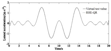
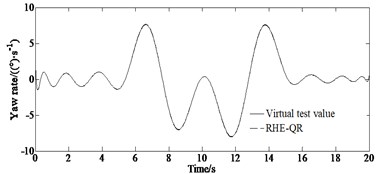
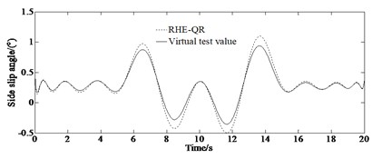
Fig. 4 contains the simulation results of the lateral acceleration, yaw rate and side slip angle.

Fig. 4Simulation results: a) lateral acceleration, b) yaw rate, c) side slip angle

a)

b)

c)

Combining with the lateral acceleration response curve in Fig. 4(a), it can be seen that when the vehicle is driving at the turning point under the double lane change condition, with the sudden increase of the steering wheel angle, the lateral acceleration increases significantly, and there is a risk of losing the stability. It can be seen from Fig. 4(b) that the RHE-QR algorithm can better track the reference value of the yaw rate output by the virtual experiment. It can be seen from Fig. 4(c) that in the initial stage and the end stage of the double lane change condition, the proposed estimation algorithm can achieve a good estimation result. But when the vehicle is running at turning of the double lane change road, due to a sudden change of steering wheel angle at this time, the driving state of the vehicle tends to be unstable, but the RHE-QR algorithm can still better track the reference value of the side slip angle.

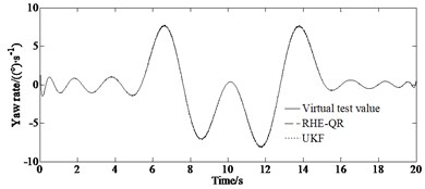
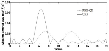
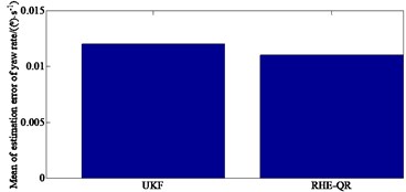
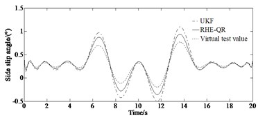
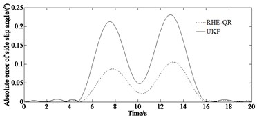
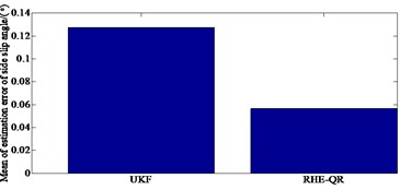
Fig. 5 depicts the comparison results of the yaw rate and the side slip angle studied with the different methods (RHE-QR and UKF) for passing a double lane change road maneuver.

From Fig. 5, it can be seen that the accuracy of the RHE-QR estimation method is significantly higher than that of the UKF method. Compared with the traditional UKF updating method, the updating arrival cost with QR decomposition has a higher accuracy while the simulation condition is similar. This is due to the fact that the updating arrival cost with the strategy of QR decomposition utilizes the results of RHE-QR estimation method to form a feedback mechanism, and updates the arrival cost by directly solving the optimization problem. It has the potential for practical application. Finally, the model ignores the effects of suspension dynamics and wheel camber. However, the RHE-QR algorithm limits the excessive increase of arrival cost and guarantees the stability of moving horizon estimation algorithm.

Fig. 5Comparison results of key variables simulated with UKF method: a) yaw rate, b) absolute error of yaw rate, c) mean of estimation of yaw rate, d) side slip angle, e) absolute error of side slip angle, f) mean of estimation error of side slip angle

Comparison results of key variables simulated with UKF method: a) yaw rate, b) absolute error of yaw rate, c) mean of estimation of yaw rate, d) side slip angle, e) absolute error of side slip angle, f) mean of estimation error of side slip angle

a)

b)

c)

d)

e)

f)

4.2. Experimental verification

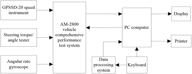
According to BS ISO 3888-2002, a double lane change test is carried out to verify the effectiveness of the algorithm collecting the yaw rate and lateral acceleration as well as the side slip angle of the vehicle. It is very dangerous to establish a real vehicle test on a double lane change road with a higher speed than 45 km/h. This speed is set up as the optimal in terms of the driver’s safety. A block diagram of real vehicle test system is shown in Fig. 6.

Fig. 6Block diagram of test system

And the main measurement devices are shown in Fig. 7. And the real test vehicle which photos are taken on the test grounds of is shown in Fig. 8.

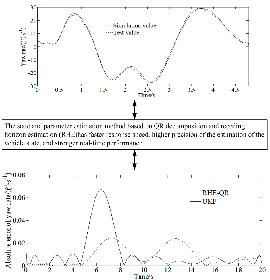
Fig. 9 depicts a comparison of the estimated and test values.

Fig. 7Measurement devices: a) GPSSD-20 speed instrument, b) steering torque/angle tester, c) AM-2800 vehicle comprehensive performance test system

a)

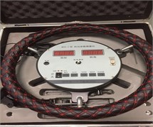
b)

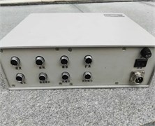
c)

Fig. 8Real test vehicle

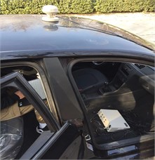
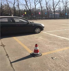
Fig. 9Comparison of estimated and test values: a) longitudinal velocity, b) lateral acceleration, c) yaw rate, d) absolute error of yaw rate

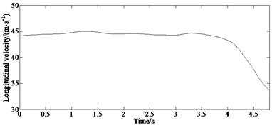
a)

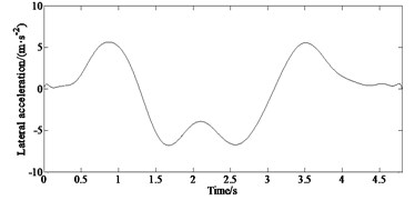
b)

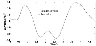
c)

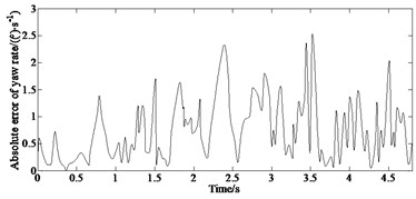
d)

The results of the double lane change test are shown in Fig. 9. It can be seen from Fig. 9(a) that the vehicle speed decreased during the double lane change operation, and the vehicle speed is 34 km·h^-1 when the test is completed. It can be seen from Figs. 9(c-d) that the overall error of the yaw rate obtained based on the RHE-QR estimation algorithm proposed in this paper and measured by gyroscope is small. Combining with the lateral acceleration response curve in Fig. 9(b), it can be seen that when the vehicle is driving through a turning point under the double lane change condition, with the sudden increase of the steering angle, the lateral acceleration increases significantly, greater than 0.4 g which indicates that the vehicle is in nonlinear state having the risk of losing stability. Due to the existence of the vehicle dynamics model, tire model and sensor measurement errors, the estimated error of the yaw rate is relatively increased, but the error returns to a smaller range thereafter. The overall estimation effect is good, and it maintains a good consistency with the actual measured value. In conclusion, the RHE-QR estimation algorithm proposed in this paper has good estimation accuracy and robustness.

5. Conclusions

In this paper, a vehicle state and parameter estimation method are proposed. Firstly, based on the 3-DOF vehicle model and the magic formula tire model, aiming at the characteristics of nonlinearity, uncertainty and rigid body/elasticity coupling of vehicle, a joint state and parameter estimation method based on QR decomposition and receding horizon estimation is proposed. Based on the MATLAB simulation platform, the state and parameter estimation algorithm proposed in this paper is verified in the double lane change condition, and compared with the UKF estimation algorithm. The simulation results show that the maximum errors between the estimated values of the side slip angle and yaw rate obtained by the estimation algorithm proposed in this paper and the reference values taken from a virtual experiment are smaller than the estimated values of the UKF algorithm. Especially when the vehicle is in a strong nonlinear state, the reference value can still be tracked well, which provides a guarantee for vehicle stability control under extreme conditions. The test results show that the estimated yaw rate value and the actual measured value can maintain a good consistency indicating good estimation accuracy.

This paper only estimates the lateral acceleration and the side slip angle as well as the yaw rate, but there are many factors that affect the driving stability of the vehicle, such as tire lateral force, longitudinal force and so on, which were ignored in this paper. That is why, due to the limitation of test conditions, only the accuracy of yaw rate estimation can be verified. Therefore, the estimation of tire lateral force, longitudinal force and other state variables as well as real vehicle test will be the focus of future research.

References

Y. Wang, L. Xu, F. Zhang, H. Dong, Y. Liu, and G. Yin, “An adaptive fault-tolerant EKF for vehicle state estimation with partial missing measurements,” IEEE/ASME Transactions on Mechatronics, Vol. 26, No. 3, pp. 1318–1327, Jun. 2021, https://doi.org/10.1109/tmech.2021.3065210

Publisher
I. Hashlamon, “A new adaptive extended Kalman filter for a class of nonlinear systems,” Journal of Applied and Computational Mechanics, Vol. 6, No. 1, pp. 1–12, Jan. 2020, https://doi.org/10.22055/jacm.2019.28130.1455

Publisher
X. Wang, A. Wang, D. Wang, Y. Xiong, B. Liang, and Y. Qi, “A modified Sage-Husa adaptive Kalman filter for state estimation of electric vehicle servo control system,” in Energy Reports, Vol. 8, pp. 20–27, Aug. 2022, https://doi.org/10.1016/j.egyr.2022.02.105

Publisher
Y. Liang, S. Muller, D. Schwendner, D. Rolle, D. Ganesch, and I. Schaffer, “A scalable framework for robust vehicle state estimation with a fusion of a low-cost IMU, the GNSS, radar, a camera and lidar,” in 2020 IEEE/RSJ International Conference on Intelligent Robots and Systems (IROS), pp. 1661–1668, Oct. 2020, https://doi.org/10.1109/iros45743.2020.9341419

Publisher
G. Park, S. B. Choi, D. Hyun, and J. Lee, “Integrated observer approach using in-vehicle sensors and GPS for vehicle state estimation,” Mechatronics, Vol. 50, pp. 134–147, Apr. 2018, https://doi.org/10.1016/j.mechatronics.2018.02.004

Publisher
Z. Yu, X. Hou, B. Leng, and Y. Huang, “Mass estimation method for intelligent vehicles based on fusion of machine learning and vehicle dynamic model,” Autonomous Intelligent Systems, Vol. 2, No. 1, pp. 1–10, Dec. 2022, https://doi.org/10.1007/s43684-022-00020-8

Publisher
Y. Zhang, J. Ma, X. Zhao, X. Liu, and K. Zhang, “A modified unscented Kalman filter combined with ant lion optimization for vehicle state estimation,” Mathematical Problems in Engineering, Vol. 2021, pp. 1–21, Jan. 2021, https://doi.org/10.1155/2021/8847075

Publisher
R. Song and Y. Fang, “Vehicle state estimation for INS/GPS aided by sensors fusion and SCKF-based algorithm,” Mechanical Systems and Signal Processing, Vol. 150, p. 107315, Mar. 2021, https://doi.org/10.1016/j.ymssp.2020.107315

Publisher
Y. Zhang, X. Wang, S. Wang, and X. Tian, “Distributed bearing-based formation control of unmanned aerial vehicle swarm via global orientation estimation,” Chinese Journal of Aeronautics, Vol. 35, No. 1, pp. 44–58, Jan. 2022, https://doi.org/10.1016/j.cja.2021.05.009

Publisher
Y.-J. Liu, C.-H. Dou, F. Shen, and Q.-Y. Sun, “Vehicle state estimation based on unscented Kalman filtering and a genetic-particle swarm algorithm,” Journal of The Institution of Engineers (India): Series C, Vol. 102, No. 2, pp. 447–469, Apr. 2021, https://doi.org/10.1007/s40032-021-00663-1

Publisher
Y. J. Liu and C. H. Dou, “Vehicle state estimation based on unscented Kalman filtering and a genetic algorithm,” SAE International Journal of Commercial Vehicles, Vol. 14, No. 1, pp. 1–15, 2021, https://doi.org/10.19562/j.chinasae.qcgc.2019.02.012

Publisher
K. Yang, Y. Tang, and Z. Zhang, “Parameter identification and state-of-charge estimation for lithium-ion batteries using separated time scales and extended Kalman filter,” Energies, Vol. 14, No. 4, p. 1054, Feb. 2021, https://doi.org/10.3390/en14041054

Publisher
O. A. Shereena and B. N. Rao, “Combined road roughness and vehicle parameter estimation based on a minimum variance unbiased estimator,” International Journal of Structural Stability and Dynamics, Vol. 20, No. 1, p. 2050013, Jan. 2020, https://doi.org/10.1142/s0219455420500133

Publisher
T. Chen et al., “Design and verification for vehicle longitudinal force and sideslip angle hierarchical estimation method,” Journal of Xi’an Jiaotong University, Vol. 53, No. 11, pp. 131–140, 2019, https://doi.org/10.7652/xjtuxb201911019

Publisher
H. Liu, P. Wang, J. Lin, H. Ding, H. Chen, and F. Xu, “Real-time longitudinal and lateral state estimation of preceding vehicle based on moving horizon estimation,” IEEE Transactions on Vehicular Technology, Vol. 70, No. 9, pp. 8755–8768, Sep. 2021, https://doi.org/10.1109/tvt.2021.3100988

Publisher
X. Sun, W. Hu, Y. Cai, P. K. Wong, and L. Chen, “Identification of a piecewise affine model for the tire cornering characteristics based on experimental data,” Nonlinear Dynamics, Vol. 101, No. 2, pp. 857–874, Jul. 2020, https://doi.org/10.1007/s11071-020-05846-6

Publisher
B. Gao, G. Hu, Y. Zhong, and X. Zhu, “Cubature Kalman filter with both adaptability and robustness for tightly-coupled GNSS/INS integration,” IEEE Sensors Journal, Vol. 21, No. 13, pp. 14997–15011, Jul. 2021, https://doi.org/10.1109/jsen.2021.3073963

Publisher
B. Gao, G. Hu, Y. Zhong, and X. Zhu, “Cubature rule-based distributed optimal fusion with identification and prediction of kinematic model error for integrated UAV navigation,” Aerospace Science and Technology, Vol. 109, p. 106447, Feb. 2021, https://doi.org/10.1016/j.ast.2020.106447

Publisher
B. Guo, N. Guo, and Z. Cen, “Obstacle avoidance with dynamic avoidance risk region for mobile robots in dynamic environments,” IEEE Robotics and Automation Letters, Vol. 7, No. 3, pp. 5850–5857, Jul. 2022, https://doi.org/10.1109/lra.2022.3161710

Publisher
A. Habibnejad Korayem, E. Hashemi, A. Khajepour, and B. Fidan, “Estimation of vehicle-trailer hitch-forces and lateral tire forces independent of trailer type and geometry,” Journal of Dynamic Systems, Measurement, and Control, Vol. 144, No. 5, pp. 1–12, May 2022, https://doi.org/10.1115/1.4053612

Publisher
X. Chen, S. Li, L. Li, W. Zhao, and S. Cheng, “Longitudinal-lateral-cooperative estimation algorithm for vehicle dynamics states based on adaptive-square-root-cubature-Kalman-filter and similarity-principle,” Mechanical Systems and Signal Processing, Vol. 176, p. 109162, Aug. 2022, https://doi.org/10.1016/j.ymssp.2022.109162

Publisher
E. K. Chen, W. X. Xing, and C. S. Gao, “State and parameter moving horizon estimation for elastic hypersonic vehicles,” Journal of Beijing University of Aeronautics and Astronautics, Vol. 45, No. 2, pp. 291–298, 2019, https://doi.org/10.13700/j.bh.1001-5965.2018.0273

Publisher
C. V. Rao, J. B. Rawlings, and D. Q. Mayne, “Constrained state estimation for nonlinear discrete-time systems: stability and moving horizon approximations,” IEEE Transactions on Automatic Control, Vol. 48, No. 2, pp. 246–258, Feb. 2003, https://doi.org/10.1109/tac.2002.808470

Publisher

About this article

Received

02 July 2022

Accepted

24 October 2022

Published

23 December 2022

SUBJECTS

Vibration in transportation engineering

DOI

https://doi.org/10.21595/jve.2022.22795

Keywords

automotive engineering

vehicle state estimation

receding horizon estimation

QR decomposition

Acknowledgements

This research was supported by the Science and Technology Program Foundation of Weifang under Grant 2015GX007. And also, this research was financially supported by the Open Research Fund from the State Key Laboratory of Rolling and Automation, Northeastern University, under Grant 2021RALKFKT008. The first author gratefully acknowledges the support agency.

Data Availability

The datasets generated during and/or analyzed during the current study are available from the corresponding author on reasonable request.

Conflict of interest

The authors declare that they have no conflict of interest.

This is an open access article distributed under the Creative Commons Attribution License, which permits unrestricted use, distribution, and reproduction in any medium, provided the original work is properly cited.

Previous article in issue Previous Next article in issue Next

Research article

2023 11 18

Vehicle state and parameter estimation based on adaptive anti-outlier unscented Kalman filter and GA-BPNN method

Yingjie Liu, Dawei Cui, Wen Peng

Research article

2023 10 30

Vehicle state and parameter estimation based on improved extend Kalman filter

Yingjie Liu, Dawei Cui, Wen Peng

Research article

2022 12 11

Vehicle state and parameter estimation based on adaptive robust unscented particle filter

Yingjie Liu, Dawei Cui, Wen Peng

Research article

2022 08 15

Vehicle state and parameter estimation based on double cubature Kalman filter algorithm

Yingjie Liu, Dawei Cui

Y. Liu, D. Cui, and W. Peng, “Moving horizon estimation of vehicle state and parameters,” Journal of Vibroengineering, Vol. 25, No. 2, pp. 409–427, Dec. 2022, https://doi.org/10.21595/jve.2022.22795

Copy Extrica

Copied to clipboard!

TY  - JOUR
DO  - 10.21595/jve.2022.22795
UR  - https://doi.org/10.21595/jve.2022.22795
TI  - Moving horizon estimation of vehicle state and parameters
T2  - Journal of Vibroengineering
AU  - Liu, Yingjie
AU  - Cui, Dawei
AU  - Peng, Wen
PY  - 2022
DA  - 2022/12/23
PB  - JVE International Ltd.
SP  - 409-427
VL  - 25
IS  - 2
SN  - 1392-8716
SN  - 2538-8460
ER  - 

Copy Ris

Copied to clipboard!

@article{Liu_2022,
	doi = {10.21595/jve.2022.22795},
	url = {https://doi.org/10.21595/jve.2022.22795},
	year = 2022,
	month = {dec},
	publisher = {{JVE} International Ltd.},
	volume = {25},
	number = {2},
	pages = {409--427},
	author = {Yingjie Liu and Dawei Cui and Wen Peng},
	title = {Moving horizon estimation of vehicle state and parameters},
	journal = {Journal of Vibroengineering}
}

Copy Bibtex

Copied to clipboard!

[1]Y. Liu, D. Cui, and W. Peng, “Moving horizon estimation of vehicle state and parameters,” Journal of Vibroengineering, vol. 25, no. 2, pp. 409–427, Dec. 2022, doi: 10.21595/jve.2022.22795.

Copy IEEE

Copied to clipboard!

Liu, Yingjie, Dawei Cui, and Wen Peng. “Moving Horizon Estimation of Vehicle State and Parameters.” Journal of Vibroengineering 25, no. 2 (December 23, 2022): 409–27. https://doi.org/10.21595/jve.2022.22795.

Copy Chicago

Copied to clipboard!

Moving horizon estimation of vehicle state and parameters

Abstract

Highlights

1. Introduction

2. Mathematical model of vehicle dynamics

2.1. 3-DOF vehicle model

2.2. Tire dynamic model

2.3. Nonlinear vehicle system

3. Receding horizon estimation based on QR decomposition

3.1. Problem description

3.2. Arrival cost calculation method of based on QR decomposition

3.3. Solution of rolling horizon estimation problem

4. Numerical simulation and experimental verification

4.1. Numerical simulation

4.1.1. Chassis model

4.1.2. Body system model

4.1.3. Powertrain system model

4.1.4. Steering system

4.1.5. Suspension system

4.2. Experimental verification

5. Conclusions

References

About this article

Related Articles