Vehicle state and parameter estimation based on improved extend Kalman filter

Liu, Yingjie; Cui, Dawei; Peng, Wen

doi:10.21595/jme.2023.23475

Journal of Measurements in Engineering

Browse Journal

Submit article

Published: 30 October 2023

Check for updates

Vehicle state and parameter estimation based on improved extend Kalman filter

Yingjie Liu¹

Dawei Cui²

Wen Peng³

^{1, 2}School of Machinery and Automation, Weifang University, Weifang, 261061, Shandong, China

³State Key Laboratory of Rolling and Automation, Northeastern University, Shenyang, 110819, China

Corresponding Author:

Yingjie Liu

Cite the article Download PDF

Downloads 93

Abstract

In order to reduce the influence of historical measurement data errors in the process of vehicle state estimation and improve the accuracy of the vehicle state estimation, a limited memory random weighted extended Kalman filter (LMRWEKF) algorithm is proposed. Firstly, a 3-DOF nonlinear vehicle dynamics model is established. Secondly, the limited memory extended Kalman filter is formed by fusing the limited memory filter and the extended Kalman filter. Then, according to the random weighting theory, the weighting coefficients that obey Dirichlet distribution are introduced to further improve the filtering estimation accuracy. Finally, a virtual test based on the ADAMS/CAR is used for the experimental verification. The results show that the error in the longitudinal velocity and the yaw rate is small, especially in the mean value of estimation error of side slip angle which is different in just 0.015 degrees between the virtual test and the simulation result. And also, the results compared with traditional methods indicate that the proposed LMRWEKF algorithm can solve the problem of vehicle state estimation with the performance of noise fluctuation suppression and higher estimation accuracy. The mean absolute error (MAE) and root mean square error (RMSE) are considered to verify the estimation accuracy of the proposed algorithm. And the comparison results indicate that the estimation accuracy of the LMRWEKF algorithm is significantly higher than those of the EKF and DEKF methods.

Vehicle state and parameter estimation based on improved extend Kalman filter

Highlights

The proposed LMRWEKF algorithm can solve the problem of vehicle state estimation with the performance of noise fluctuation suppression and higher estimation accuracy.
The error in the longitudinal velocity and the yaw rate is small, especially in the mean value of estimation error of side slip angle which is different in just 0.015 degrees between the virtual test and the simulation result.
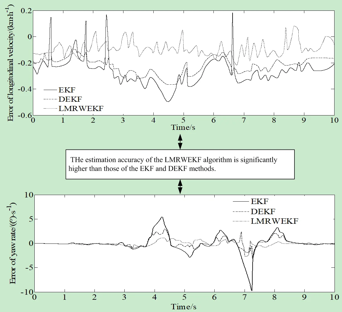
The estimation accuracy of the LMRWEKF algorithm is significantly higher than those of the EKF and DEKF methods.

1. Introduction

With the development of science and technology, vehicle active safety system has been proved to be one of the most effective ways to reduce traffic accidents. Accurate acquisition of vehicle status information is an important prerequisite for the effective operation of active safety system. However, due to some limitations of up-to-date measurement technology, current on-board sensors cannot directly measure the comprehensive vehicle status information. To solve this problem, it is possible to use expensive sensors for measurements. But because of the high cost of this method, it is difficult to meet the needs of mass production, and it remained only in the experimental stage. Another method is to combine the existing on-board sensors and use some advanced filters, observers, etc. to construct an algorithm which permits to measure, analyze and output the comprehensive vehicle state information [1]. The latter has become the focus of many experts and scholars because of its advantages such as low cost, easy operation, accurate estimation, etc. Vehicle state estimation based on vehicle kinematics model has excellent robustness, and can ignore the impact of changes in vehicle model parameters. But this method has very high requirements for the installation, calibration and accuracy of the sensor. Vehicle state estimation based on vehicle dynamics model requires less sensors, but the system model itself should reflect the vehicle dynamics characteristics as accurately as possible, and the inaccuracy of noise statistical characteristics will also affect the accuracy of state estimation [1, 2].

The problem of vehicle state estimation has been widely studied in previous researches. A brief review is presented in what follows.

Mo et al. proposed a framework of vehicle-infrastructure cooperative perception for the cooperative automated driving system to overcome the technical bottlenecks and limitations of autonomous vehicles on the information perception [3]. Kemsaram et al. presented a design model of a stereo vision system for cooperative automated vehicles based on the object-oriented analysis and design methodologies [4]. Yin et al. proposed to approximate the optimal filter gain by considering the effect factors within the infinite time horizon, on the basis of estimation-control duality [5]. Zhang et al. estimated the structure and motion of a moving object by an uncalibrated vehicle-mounted two-camera system [6]. Hao et al. investigated an asynchronous information fusion issue for a camera and radar in an intelligent driving system [7]. In order to improve the tracking and estimation accuracy, Gao et al. proposed the method of Generalized Group Lasso [8]. Galanido et al. estimated the hydrogen fuel filling time for hydrogen-powered fuel cell electric vehicles at different initial conditions through a dynamic simulation by using Aspen Dynamics v.11 with the Peng-Robinson equation of state for creating a thermodynamic model [9]. Soltani et al. presented an integrated control of longitudinal, yaw and lateral vehicle dynamics using active front steering and active braking systems [10]. Liang et al. proposed a framework to exploit the advantages of each individual sensor type to reach high accuracy and robustness [11]. Xiong et al. proposed G-VIDO, a vehicle dynamics, and intermittent Global Navigation Satellite System (GNSS)-aided visual-inertial state estimator, to address the state estimation problem of autonomous vehicle localization under various GNSS states [12]. Wang et al. developed a LiDAR-based estimation method to identify simultaneously the pose and the velocity information of an ego vehicle and its surrounding moving obstacles [13]. Li et al. presented a unified framework for concurrent dynamic multi-object joint perception [14]. Rout et al. proposed two dynamic sparsity-based state estimation approaches for distribution systems [15]. Xu et al. presented a novel dynamic vehicle tracking framework, achieving accurate pose estimation and tracking in urban environments [16]. Gao et al.proposed a new methodology to address the problem of tightly coupled GNSS/INS integration [17, 18].

The accurate acquisition of vehicle key state information is crucial to the vehicle stability control, vehicle active safety system, etc. The extended Kalman filter combined with the limited memory algorithm can solve well the impact of historical measurement data errors. Despite there were a lot of vehicle state estimation researches, they only slightly covered the extended Kalman filter combined with the limited memory filter and random weighting idea. Therefore, this paper proposes an algorithm based on the limited memory random weighted extended Kalman filter, which combines the extended Kalman filter algorithm with the limited memory filter. It improves the utilization of new measured values in the filtering estimation process, reduces the impact of old measurement data errors, and effectively improves the accuracy of the filtering algorithm. The MAE and RMSE are used to verify the estimation accuracy of the proposed algorithm.

2. Mathematical model of vehicle state estimation problem

2.1. 3-DOF vehicle model

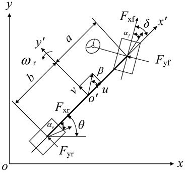
The vehicle state estimation model is established based on a 3-DOF vehicle model. The 3-DOF vehicle model is shown in Fig. 1. The vehicle coordinate system contains two axes $m$ , and the origin of the vehicle coordinate system coincides with the center of mass of the vehicle.

The dynamic equation of the 3-DOF vehicle model is as follows (Eqs. 1-4) [19]:

1

{\dot{ω}}_{r} = \frac{a^{2} k_{1} + b^{2} k_{2}}{I_{z}} \frac{ω_{r}}{u} + \frac{a k_{1} - b k_{2}}{I_{z}} β - \frac{a k_{1}}{I_{z}} δ,

2

\dot{β} = \frac{a k_{1} - b k_{2} - m u^{2}}{m} \frac{ω_{r}}{u^{2}} + \frac{k_{1} + k_{2}}{m} \frac{β}{u} - \frac{k_{1} δ}{m u},

3

\dot{u} = a_{x} + v x,

4

a_{y} = \frac{a k_{1} - b k_{2}}{m u} ω_{r} + \frac{k_{1} + k_{2}}{m} β - \frac{k_{1}}{m} δ,

where, $u$ and $v$ are the longitudinal and the lateral velocities; $ω_{r}$ is the yaw rate, $a_{x}$ and $a_{y}$ are the longitudinal and lateral accelerations; $I_{z}$ is the moment of inertia around the $z$ axis of the vehicle; $a$ and $b$ are the distances from the center of gravity to the front and rear axles; $m$ is the vehicle mass; $δ$ is the front steering angle; $k_{1}$ and $k_{2}$ are the synthesized stiffness values of front and rear tire, $s$ and $x$ is the horizontal coordinate of the body-fixed reference frame.

The side slip angle of the center of mass is Eq. (5):

5

β = a r c t a n (\frac{v}{u}) .

Fig. 13-DOF vehicle model (θ is the heading angle of the vehicle; x'o'y' is the vehicle coordinate system; Fxf and Fxr are the longitudinal forces of the front and rear tires)

3-DOF vehicle model (θ is the heading angle of the vehicle; x'o'y' is the vehicle coordinate system; Fxf and Fxr are the longitudinal forces of the front and rear tires)

2.2. Tire model

The lateral forces of front and rear wheels can be expressed as Eq. (6) [19]:

6

\{\begin{array}{l} F_{y f} = c_{f} α_{f}, \\ F_{y r} = c_{r} α_{r}, \end{array}

where $c_{f}$ and $c_{r}$ are the lateral stiffness values of the front and rear tires. $α_{f}$ and $α_{r}$ are the front and rear slip angles Eq. (7):

7

\{\begin{array}{l} c_{f} = \frac{\partial F_{y f}}{\partial α_{f}}| α_{f} = 0, \\ c_{r} = \frac{\partial F_{y r}}{\partial α_{r}}| α_{r} = 0 . \end{array}

3. Vehicle state estimation algorithm based on LMRWEKF

3.1. State space equation model

The state and measurement equation of the 3-DOF nonlinear vehicle system is established by consolidating Eqs. (1)-(4) Eq. (8):

8

\{\begin{array}{l} \dot{x} (t) = f (x (t), u (t), w (t)), \\ z (t) = h (x (t), v (t)) . \end{array}

The state and measurement variables are $x (t) = [ω, β, v_{x}]^{T}$ and $z (t) = [a_{y}]$ respectively; the system input is $u = [δ, a_{x}]^{T}$ . $f$ is the state transition function; $h$ is the measurement function; $w (t)$ and $v (t)$ are process and observation noises, and their sequences are independent of each other.

3.2. Algorithm design of LMRWEKF

3.2.1. Random weighted estimation

It is assumed that $(σ_{1}, σ_{2}, \dots, σ_{n})$ is an independent identically distributed sample from the distribution function $G (x)$ , and the empirical distribution function is Eq. (9) [20]:

9

G (x) = \frac{1}{n} \sum_{i = 1}^{N} I_{X_{i} \leq x},

where, $I_{X_{i} \leq x}$ is the indicating function, $I_{X_{i} \leq x} = \{\begin{array}{l} 1, X_{i} \leq x, \\ 0, X_{i} > x, \end{array}$ ; $n$ is the number of samples.

Then the random weighted estimate of $G (x)$ is:

10

L_{n} (x) = \sum_{i = 1}^{N} σ_{i} I_{X_{i} \leq x} .

The random weighting vector $(σ_{1}, σ_{2}, \dots, σ_{n})$ obeys the Dirichlet distribution. That is, the joint density function of $(σ_{1}, σ_{2}, \dots, σ_{n})$ satisfying $\sum_{i = 1}^{N} σ_{i} = 1$ is:

11

g (σ_{1}, σ_{2}, \dots, σ_{n}) = Θ (n),

where $(σ_{1}, σ_{2}, \dots, σ_{n}) \in D_{n - 1},$ and $D_{n - 1} = {(σ_{1}, σ_{2}, \dots, σ_{n - 1}) : σ_{i} \geq 0, i = 1,2, \dots, n - 1,$ $\sum_{i = 1}^{n} σ_{i} \leq 1\}$ .

3.2.2. Limited memory filtering

The traditional memory growing filter is an infinitely increasing storage filter. If the optimal estimation is to be performed at time $k$ , then all data before time $k - 1$ should be used. This means that the proportion of old data in the filter will increase with time, while the weight of new measured data will be relatively reduced. When the noise characteristics are unknown, the error will be too large, and the estimation will be inaccurate or even divergent. Therefore, by using the idea of limited memory filter, only $N - 1$ observations at the current time and before are selected for the optimal estimation calculation that allows avoiding the above problems.

3.2.3. LMRWEKF algorithm

The LMRWEKF algorithm is proposed based on the EKF.

For the discrete state and measurement equations, the following equation is used:

12

\{\begin{array}{l} X_{k} = A_{k |k - 1} X_{k - 1} + B_{k |k - 1} U_{k - 1} + W_{k - 1}, \\ Z_{k} = H_{k} X_{k} + V_{k}, \end{array}

where $X_{k - 1}$ and $X_{k}$ are the state variable matrices of $k - 1$ and $k$ time respectively. $U_{k - 1}$ is the control variable matrix at $k - 1$ time; $Z_{k}$ is the measurement output matrix at time $k$ ; $A_{k |k - 1}$ is the state transition matrix of $k - 1$ to predict $k$ time; $B_{k |k - 1}$ is the control matrix for $k - 1$ time to predict $k$ time; $H_{k}$ is the observation matrix at time $k$ ; $W_{k - 1}$ is the process noise matrix at $k - 1$ time; $V_{k}$ is the observation noise matrix at time $k$ .

The basic processing flow is:

Step 1: The initial value ${\hat{X}}_{k - 1}^{*}$ and its covariance matrix $P_{k - 1}^{*}$ are memorized.

Step 2: Prediction of state equation is made:

13

{\bar{X}}_{k} = A_{k |k - 1} {\hat{X}}_{k - 1}^{*} .

Step 3: The state transition matrix and the observation matrix are linearized:

14

\{\begin{array}{l} A \to A^{*}, \\ H \to H^{*} . \end{array}

Step 4: Prediction of the covariance matrix is made:

15

P_{k |k - 1}^{*} = A_{k |k - 1}^{*} P_{k - 1}^{*} A_{k |k - 1}^{* T} + Q_{k - 1},

where $Q_{k - 1}$ is the covariance matrix of process noise at time $k - 1$ .

Step 5: Prediction of the observation equation is made:

16

{\bar{Z}}_{k} = H_{k} {\bar{X}}_{k} .

Step 6: The observation error is calculated:

17

r_{k} = Z_{k} - {\bar{Z}}_{k} .

Step 7: If $k \leq N$ , then ${\hat{R}}_{k}^{*} = R$ . If $k > N$ , then ${\hat{r}}_{k}^{*} = \sum_{i = k - N + 1}^{k} σ_{i} r_{i} = \sum_{i = k - N + 1}^{k} \frac{1 - ε}{1 - ε^{N}} ε^{k - i} r_{i}$ , where $σ_{i} = \frac{1 - ε}{1 - ε^{N}} ε^{k - i}$ obeys the Dirichlet distribution; $ε$ is the weighting coefficient and $ε \in [0.95,0.995]$ (Eq. 18):

18

{\hat{R}}_{k}^{*} r = \sum_{i = k - N + 1}^{k} σ_{i} [(r_{i} - {\hat{r}}_{k}^{*}) (r_{i} - {\hat{r}}_{k}^{*})^{T} - \frac{N - 1}{N} H_{k}^{*} P_{k |k - 1}^{*} H_{k}^{* T}] .

Step 8: The filter gain is calculated:

19

K_{k}^{*} = P_{k |k - 1}^{*} H_{k}^{* T} (H_{k}^{*} P_{k |k - 1}^{*} H_{k}^{* T} + {\hat{R}}_{k}^{*})^{- 1} .

Step 9: The status is updated:

20

{\hat{X}}_{k}^{*} = {\bar{X}}_{k} + K_{k}^{*} (Z_{k} - H_{k} {\bar{X}}_{k}) .

Step 10: The covariance matrix is updated:

21

P_{k}^{*} = (I - K_{k}^{*} H_{k}^{*}) P_{k |k - 1}^{*} (I - K_{k}^{*} H_{k}^{*})^{T} + K_{k}^{*} {\hat{R}}_{k}^{*} K_{k}^{* T},

where $I$ is the identity matrix.

Then the updating of covariance matrix is simplified:

22

\begin{array}{l} P_{k}^{*} = (I - K_{k}^{*} H_{k}^{*}) P_{k |k - 1}^{*} - P_{k |k - 1}^{*} H_{k}^{* T} K_{k}^{* T} + K_{k}^{*} H_{k}^{*} P_{k |k - 1}^{*} \cdot H_{k}^{* T} K_{k}^{* T} + K_{k}^{*} {\hat{R}}_{k}^{*} K_{k}^{* T} \\ = (I - K_{k}^{*} H_{k}^{*}) P_{k |k - 1}^{*} - P_{k |k - 1}^{*} \cdot H_{k}^{* T} K_{k}^{* T} + K_{k}^{*} (H_{k}^{*} P_{k |k - 1}^{*} H_{k}^{* T} + {\hat{R}}_{k}^{*}) K_{k}^{* T} \\ = (I - K_{k}^{*} H_{k}^{*}) P_{k |k - 1}^{*} - P_{k |k - 1}^{*} H_{k}^{* T} K_{k}^{* T} + P_{k |k - 1}^{*} H_{k}^{* T} K_{k}^{* T} = (I - K_{k}^{*} H_{k}^{*}) P_{k |k - 1}^{*} . \end{array}

4. Numerical simulation and experimental verification

4.1. Numerical simulation

In order to verify the feasibility and accuracy of the proposed algorithm, the longitudinal velocity, yaw rate, side slip angle and other related parameters of the vehicle are estimated in real time, and the estimation results are compared to verify the superiority of LMRWEKF algorithm. The vehicle dynamics simulation software Carsim in the Matlab/Simulink environment is used for simulation.

Carsim is a simulation software for calculating the vehicle dynamics. Its model runs 3~6 times faster on the computer than in the real time. This software can simulate the response of the vehicle to the driver, road and aerodynamic inputs. It is mainly used to predict and simulate the handling stability, braking performance, power performance and economy of the whole vehicle. It is also widely used in the development of modern vehicle control systems.

Carsim simulation software is composed of three parts: the graphic vehicle database, model solver and simulator for post-processing the results. Carsim dynamics software omits a series of tedious processes of modeling and debugging the structured software and user programming to establish mathematical models. Combining traditional vehicle dynamics and modern multi-body dynamics modeling methods, the software abstracts and simplifies the actual vehicle. On the basis of simplification, it calculates the vehicle characteristics and initial simulation conditions. The vehicle model in Carsim includes the body, wheels, steering, suspension, braking and transmission systems as well as aerodynamic systems. Therefore, the Carsim model can temporarily replace the actual vehicle to provide the required control input and measurement output for the algorithm in this paper. After the algorithm simulation is completed, the state simulation estimation value is compared with the corresponding Carsim output value to verify the effectiveness of the estimation algorithm. The flow chart of co-simulation of Carsim and Matlab/Simulink is shown in Fig. 2.

Fig. 2Flow chart of co-simulation of Carsim and Matlab/Simulink

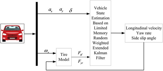
The longitudinal acceleration, lateral acceleration and steering wheel angle signals can be measured by the corresponding sensors. And the three states are taken as the input signals of the estimation module. The three input signals are shown in Fig. 3.

In order to verify the effectiveness of the proposed method, the traditional method of EKF and the classical method of dual extended Kalman filter (DEKF) proposed in Reference [21] are used to establish comparison results.

Fig. 4 shows the simulation results for a vehicle passing a double lane change road.

From Figs. 4(a) and 4(c), it can be seen that compared with the traditional EKF algorithm, the LMRWEKF algorithm can better approach the reference value, and the deviation is relatively smaller at the peak and trough of the curve, and has a strong inhibition effect on noise fluctuations. The longitudinal velocity estimation of LMRWEKF algorithm is obviously closer to the reference value than that of the traditional EKF algorithm. And when the noise characteristics are unknown, the LMRWEKF algorithm jitters less, which indicates that it has a good noise suppression effect and is more stable and robust.

Fig. 3Signal input

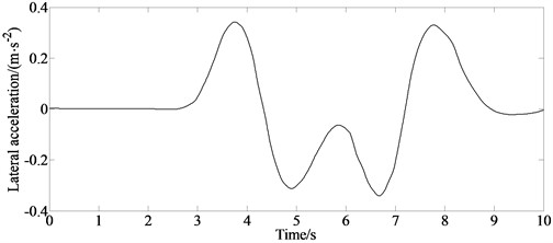
a) Lateral acceleration

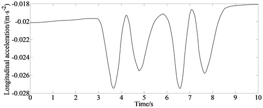
b) Longitudinal acceleration

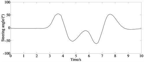
c) Steering angle

The EKF method is based on linear minimum variance estimation as the theoretical basis, and filters and estimates state variables through recursive algorithms. Although it has high estimation accuracy, it is an infinitely growing memory filter like traditional Kalman filters. Its computational efficiency and estimation accuracy will decrease over time, so the filtering algorithm cannot effectively solve the impact of model inaccuracy or unknown noise characteristics.

The DEKF method utilizes two parallel driven EKFs that interact in a “guided” manner. One advantage of this method is that through the effective and improved estimation accuracy, the model uncertainty within the state estimator is reduced, allowing for the improved quality of state estimation and reducing the uncertainty of the state estimator.

The LMRWEKF algorithm proposed in this paper can dynamically adjust the noise statistical characteristics of the filter estimation algorithm in a real time. So, it can deal with the problem of unknown noise characteristics. Its limited memory algorithm characteristics can still have faster response speed and estimation accuracy under the condition of poor computing capacity. From Figs. 4(b) and 4(d), it can be seen that the filter estimation error of LMRWEKF algorithm is lower than that of traditional EKF algorithm, and the overall estimation performance is better.

Fig. 4Simulation results for vehicle passing double lane change road

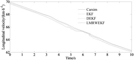
a) Longitudinal velocity

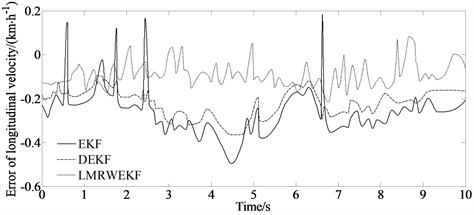
b) Error of longitudinal velocity

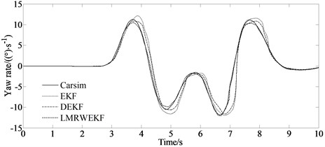
c) Yaw rate

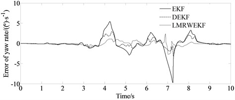
d) Error of yaw rate

The mean absolute error and root mean square error are considered to verify the estimation accuracy of the proposed algorithm.

From Table 1, it can be seen more intuitively that the estimation accuracy of the LMRWEKF algorithm is significantly higher than those of the EKF and DEKF methods.

Driving on ice snow road is a common condition for vehicles. So, it is necessary to address the simulation analysis. The initial vehicle speed of the vehicle is set as 20 km/h and the tire-road friction coefficient is set as 0.2 for the ice snow road.

The steering angle which is set as the input signal is shown in Fig. 5(a).

From Fig. 5(b), it can be seen that estimation value of LMRWEKF is closer to the reference value, indicating the good estimation performance of the LMRWUKF method.

Table 1MAE and RMSE indicators of three algorithms

Evaluation index	State value	EKF	DEKF	LMRWEKF
MAE	$v$ (m/s)	0.322	0.258	0.141
	$u$ (m/s)	0.191	0.161	0.0458
	$ω_{r}$ (rad/s)	0.325	0.319	0.0166
RMSE	$v$ (m/s)	0.355	0.302	0.136
	$u$ (m/s)	0.255	0.143	0.0509
	$ω_{r}$ (rad/s)	0.432	0.334	0.0201

Fig. 5Simulation results for vehicle passing ice snow road

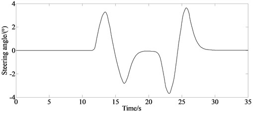
a) Input signal

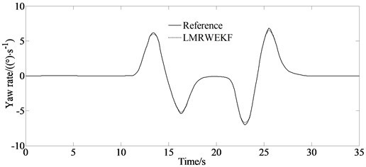
b) Yaw rate under the condition of ice snow road

4.2. Experimental verification

ADAMS/CAR software is a virtual machine simulation and analysis software developed and designed by the MSC Company from the United States. At present, it is widely used in automobile, machinery and other manufacturing industries around the world. ADAMS/CAR software can design virtual components of the whole vehicle system, such as body, suspension system , tires, etc., and simulate and analyze the virtual simulation model to compare the simulation result with the virtual experiment results close to the real test, and can output the dynamic curve in the post-processing system, and dynamically analyze the virtual simulation model as per the dynamic curve. The method of virtual model creation in the ADAMS/CAR software applied for simulation experiment has the following advantages: (1) Before the company manufactures the actual products, a model of the products can be simulated, analyzed and modified to save the testing cost of the actual products; (2) The virtual prototype is analyzed on a computer, which greatly reduces the cost of testing the actual prototype. For some researches where it can be difficult to conduct real experiments, ADAMS/CAR software can be used to complete the researches safely and efficiently, ensuring the safety of personnel and the integrity of property; (3) The simulation experiment is conducted in the ADAMS/CAR software and will not be affected by external objective factors such as weather. ADAMS/CAR has a variety of independent modules, and provides complete vehicle models of cars, trucks and buses. In the template builder mode, designers can adjust each module or create new modules, and import them into simulation experiments for use. Therefore, this paper mainly uses the template builder to modify the road module, tire module and truck module after establishing the vehicle tire road model. Finally, the vehicle tire road coupling model is simulated.

The vehicle model for simulation is shown in Fig. 6.

Fig. 6Vehicle model in ADAMS

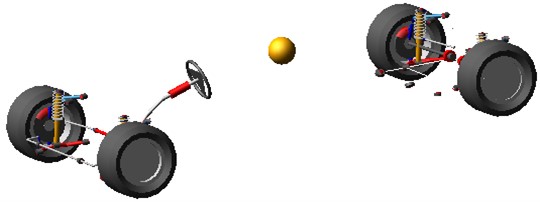
Fig. 7Virtual test and simulation results

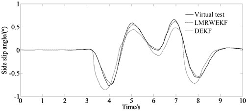
a) Side slip angle

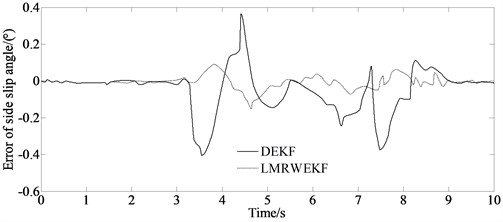
b) Error of side slip angle

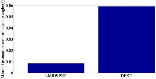
c) Mean value of estimation error of side slip angle

The results of the virtual test and the simulation are shown in Figs. 7(a) and (b) respectively.

From Fig. 7(a), it can be seen that the simulation result of the LMRWEKF algorithm can better approach the virtual test value. Moreover, from Fig. 7(b) it can be seen that the deviation is relatively smaller. At the same time, from Fig. 7(c) it can be seen that the mean value of estimation error of side slip angle is just 0.015 degrees. From the above analysis, it can be seen that the proposed algorithm has higher estimation accuracy, and the filter estimation error of LMRWEKF algorithm is lower that demonstrates that the overall estimation performance of the proposed algorithm is better.

5. Conclusions

In this paper, a nonlinear vehicle dynamics model including longitudinal, lateral and yaw degrees of freedom is established. The extended Kalman filter is combined with the limited memory filter. In the limited memory length area, the covariance matrix of the current measurement noise matrix is obtained by detecting the innovation residual sequence and using mathematical statistics, so as to reduce the estimation error caused by an inaccurate model. Based on the random weighting theory, the random weighting coefficient is introduced to improve the utilization of the filtering system by obtaining new measured values, thus improving the accuracy of the filtering algorithm and enhancing the adaptability. It has a wide range of practical applications. For example, the method can provide on-line estimation of the model parameters in autonomous vehicles. Simulation experiments show that the algorithm can effectively suppress the filtering estimation error caused by noise fluctuations, and achieve effective estimation of vehicle yaw rate, side slip angle of the center of mass, and longitudinal acceleration under the condition of unknown measurement noise characteristics. The results show that the error of the longitudinal velocity and the yaw rate is small, especially the mean value of estimation error of side slip angle which is just 0.015 degrees between the virtual test and the simulation result. The MAE and RMSE are considered to verify the estimation accuracy of the proposed algorithm. And the comparison results indicate that the estimation accuracy of the LMRWEKF algorithm is significantly higher than those of the EKF and DEKF methods.

References

Y. Liu and D. Cui, “Vehicle state and parameter estimation based on double cubature Kalman filter algorithm,” Journal of Vibroengineering, Vol. 24, No. 5, pp. 936–951, Aug. 2022, https://doi.org/10.21595/jve.2022.22356

Publisher
Y. Liu and D. Cui, “Vehicle state estimation based on adaptive fading unscented Kalman filter,” Mathematical Problems in Engineering, Vol. 2022, pp. 1–11, Apr. 2022, https://doi.org/10.1155/2022/7355110

Publisher
Y. Mo, P. Zhang, Z. Chen, and B. Ran, “A method of vehicle-infrastructure cooperative perception based vehicle state information fusion using improved Kalman filter,” Multimedia Tools and Applications, Vol. 81, No. 4, pp. 4603–4620, Feb. 2022, https://doi.org/10.1007/s11042-020-10488-2

Publisher
N. Kemsaram, A. Das, and G. Dubbelman, “A model-based design of an onboard stereo vision system: obstacle motion estimation for cooperative automated vehicles,” SN Applied Sciences, Vol. 4, No. 7, pp. 1–18, Jul. 2022, https://doi.org/10.1007/s42452-022-05078-w

Publisher
Y. Yin, S. E. Li, K. Tang, W. Cao, W. Wu, and H. Li, “Approximate optimal filter design for vehicle system through actor-critic reinforcement learning,” Automotive Innovation, Vol. 5, No. 4, pp. 415–426, Nov. 2022, https://doi.org/10.1007/s42154-022-00195-z

Publisher
X. Zhang, J. Chen, J. Deng, R. Wang, W. Xiong, and Q. Wang, “Structure and motion for intelligent vehicles using an uncalibrated two-camera system,” IEEE Transactions on Industrial Electronics, Vol. 70, No. 2, pp. 1772–1782, Feb. 2023, https://doi.org/10.1109/tie.2022.3163509

Publisher
X. Hao, Y. Xia, H. Yang, and Z. Zuo, “Asynchronous information fusion in intelligent driving systems for target tracking using cameras and radars,” IEEE Transactions on Industrial Electronics, Vol. 70, No. 3, pp. 2708–2717, Mar. 2023, https://doi.org/10.1109/tie.2022.3169717

Publisher
R. Gao, S. Sarkka, R. Claveria-Vega, and S. Godsill, “autonomous tracking and state estimation with generalized group Lasso,” IEEE Transactions on Cybernetics, Vol. 52, No. 11, pp. 12056–12070, Nov. 2022, https://doi.org/10.1109/tcyb.2021.3085426

Publisher
R. J. Galanido, L. J. Sebastian, D. O. Asante, D. S. Kim, N.-J. Chun, and J. Cho, “Fuel filling time estimation for hydrogen-powered fuel cell electric vehicle at different initial conditions using dynamic simulation,” Korean Journal of Chemical Engineering, Vol. 39, No. 4, pp. 853–864, Apr. 2022, https://doi.org/10.1007/s11814-021-0983-1

Publisher
A. Soltani, S. Azadi, and R. N. Jazar, “Integrated control of braking and steering systems to improve vehicle stability based on optimal wheel slip ratio estimation,” Journal of the Brazilian Society of Mechanical Sciences and Engineering, Vol. 44, No. 3, pp. 1–15, Mar. 2022, https://doi.org/10.1007/s40430-022-03420-2

Publisher
Y. Liang, S. Muller, and D. Rolle, “Tightly coupled multimodal sensor data fusion for robust state observation with online delay estimation and compensation,” IEEE Sensors Journal, Vol. 22, No. 13, pp. 13480–13496, Jul. 2022, https://doi.org/10.1109/jsen.2022.3177365

Publisher
L. Xiong et al., “G-VIDO: a vehicle dynamics and intermittent GNSS-aided visual-inertial state estimator for autonomous driving,” IEEE Transactions on Intelligent Transportation Systems, Vol. 23, No. 8, pp. 11845–11861, Aug. 2022, https://doi.org/10.1109/tits.2021.3107873

Publisher
Q. Wang, J. Chen, J. Deng, X. Zhang, and K. Zhang, “Simultaneous pose estimation and velocity estimation of an ego vehicle and moving obstacles using LiDAR information only,” IEEE Transactions on Intelligent Transportation Systems, Vol. 23, No. 8, pp. 12121–12132, Aug. 2022, https://doi.org/10.1109/tits.2021.3109936

Publisher
K. Li, H. Xiong, J. Liu, Q. Xu, and J. Wang, “Real-time monocular joint perception network for autonomous driving,” IEEE Transactions on Intelligent Transportation Systems, Vol. 23, No. 9, pp. 15864–15877, Sep. 2022, https://doi.org/10.1109/tits.2022.3146087

Publisher
B. Rout, S. Dahale, and B. Natarajan, “Dynamic matrix completion based state estimation in distribution grids,” IEEE Transactions on Industrial Informatics, Vol. 18, No. 11, pp. 7504–7511, Nov. 2022, https://doi.org/10.1109/tii.2022.3162210

Publisher
F. Xu, Z. Wang, H. Wang, L. Lin, and H. Liang, “Dynamic vehicle pose estimation and tracking based on motion feedback for LiDARs,” Applied Intelligence, Vol. 53, No. 2, pp. 2362–2390, Jan. 2023, https://doi.org/10.1007/s10489-022-03576-3

Publisher
B. Gao, G. Hu, Y. Zhong, and X. Zhu, “Cubature Kalman filter with both adaptability and robustness for tightly-coupled GNSS/INS integration,” IEEE Sensors Journal, Vol. 21, No. 13, pp. 14997–15011, Jul. 2021, https://doi.org/10.1109/jsen.2021.3073963

Publisher
B. Gao, G. Hu, Y. Zhong, and X. Zhu, “Cubature rule-based distributed optimal fusion with identification and prediction of kinematic model error for integrated UAV navigation,” Aerospace Science and Technology, Vol. 109, p. 106447, Feb. 2021, https://doi.org/10.1016/j.ast.2020.106447

Publisher
Y. Liu and D. Cui, “Estimation algorithm for vehicle state estimation using ant lion optimization algorithm,” Advances in Mechanical Engineering, Vol. 14, No. 3, p. 168781322210858, Mar. 2022, https://doi.org/10.1177/16878132221085839

Publisher
C. You and P. Tsiotras, “Vehicle modeling and parameter estimation using adaptive limited memory joint-state UKF,” in American Control Conference, 2017.

Publisher
T. A. Wenzel, K. J. Burnham, M. V. Blundell, and R. A. Williams, “Dual extended Kalman filter for vehicle state and parameter estimation,” Vehicle System Dynamics, Vol. 44, No. 2, pp. 153–171, Feb. 2006, https://doi.org/10.1080/00423110500385949

Publisher

About this article

Received

26 June 2023

Accepted

19 October 2023

Published

30 October 2023

DOI

https://doi.org/10.21595/jme.2023.23475

Keywords

automotive engineering

vehicle dynamics

limited memory random weighted extended Kalman filter

vehicle state estimation

Acknowledgements

This research was supported by the Science and Technology Program Foundation of Weifang under Grant 2015GX007. And also, this research was financially supported by the Open Research Fund from the State Key Laboratory of Rolling and Automation, Northeastern University, under Grant 2021RALKFKT008. The first author gratefully acknowledges the agency support.

Data Availability

The datasets generated during and/or analyzed during the current study are available from the corresponding author on reasonable request.

Author Contributions

Yingjie Liu: mathematical model and the simulation techniques. Dawei Cui: spelling and grammar checking as well as virtual validation. Wen Peng: virtual validation.

Conflict of interest

The authors declare that they have no conflict of interest.

This is an open access article distributed under the Creative Commons Attribution License, which permits unrestricted use, distribution, and reproduction in any medium, provided the original work is properly cited.

Previous article in issue Previous Next article in issue Next

Research article

2022 12 23

Moving horizon estimation of vehicle state and parameters

Yingjie Liu, Dawei Cui, Wen Peng

Research article

2022 12 11

Vehicle state and parameter estimation based on adaptive robust unscented particle filter

Yingjie Liu, Dawei Cui, Wen Peng

Research article

2022 08 15

Vehicle state and parameter estimation based on double cubature Kalman filter algorithm

Yingjie Liu, Dawei Cui

Research article

2018 05 22

Complex approach to computations and analysis of vehicle dynamics

Petr Porteš, Lubor Zháňal, Jan Fojtášek

Y. Liu, D. Cui, and W. Peng, “Vehicle state and parameter estimation based on improved extend Kalman filter,” Journal of Measurements in Engineering, Vol. 11, No. 4, pp. 496–508, Oct. 2023, https://doi.org/10.21595/jme.2023.23475

Copy Extrica

Copied to clipboard!

TY  - JOUR
DO  - 10.21595/jme.2023.23475
UR  - https://doi.org/10.21595/jme.2023.23475
TI  - Vehicle state and parameter estimation based on improved extend Kalman filter
T2  - Journal of Measurements in Engineering
AU  - Liu, Yingjie
AU  - Cui, Dawei
AU  - Peng, Wen
PY  - 2023
DA  - 2023/10/30
PB  - JVE International Ltd.
SP  - 496-508
VL  - 11
IS  - 4
SN  - 2335-2124
SN  - 2424-4635
ER  - 

Copy Ris

Copied to clipboard!

 @article{Liu_2023, title={Vehicle state and parameter estimation based on improved extend Kalman filter}, volume={11}, ISSN={2424-4635}, url={https://doi.org/10.21595/jme.2023.23475}, DOI={10.21595/jme.2023.23475}, number={4}, journal={Journal of Measurements in Engineering}, publisher={JVE International Ltd.}, author={Liu, Yingjie and Cui, Dawei and Peng, Wen}, year={2023}, month=oct, pages={496–508} }

Copy Bibtex

Copied to clipboard!

[1]Y. Liu, D. Cui, and W. Peng, “Vehicle state and parameter estimation based on improved extend Kalman filter,” Journal of Measurements in Engineering, vol. 11, no. 4, pp. 496–508, Oct. 2023, doi: 10.21595/jme.2023.23475.

Copy IEEE

Copied to clipboard!

Liu, Yingjie, Dawei Cui, and Wen Peng. “Vehicle State and Parameter Estimation Based on Improved Extend Kalman Filter.” Journal of Measurements in Engineering 11, no. 4 (October 30, 2023): 496–508. https://doi.org/10.21595/jme.2023.23475.

Copy Chicago

Copied to clipboard!

Vehicle state and parameter estimation based on improved extend Kalman filter

Abstract

Highlights

1. Introduction

2. Mathematical model of vehicle state estimation problem

2.1. 3-DOF vehicle model

2.2. Tire model

3. Vehicle state estimation algorithm based on LMRWEKF

3.1. State space equation model

3.2. Algorithm design of LMRWEKF

3.2.1. Random weighted estimation

3.2.2. Limited memory filtering

3.2.3. LMRWEKF algorithm

4. Numerical simulation and experimental verification

4.1. Numerical simulation

4.2. Experimental verification

5. Conclusions

References

About this article

Related Articles