Abstract
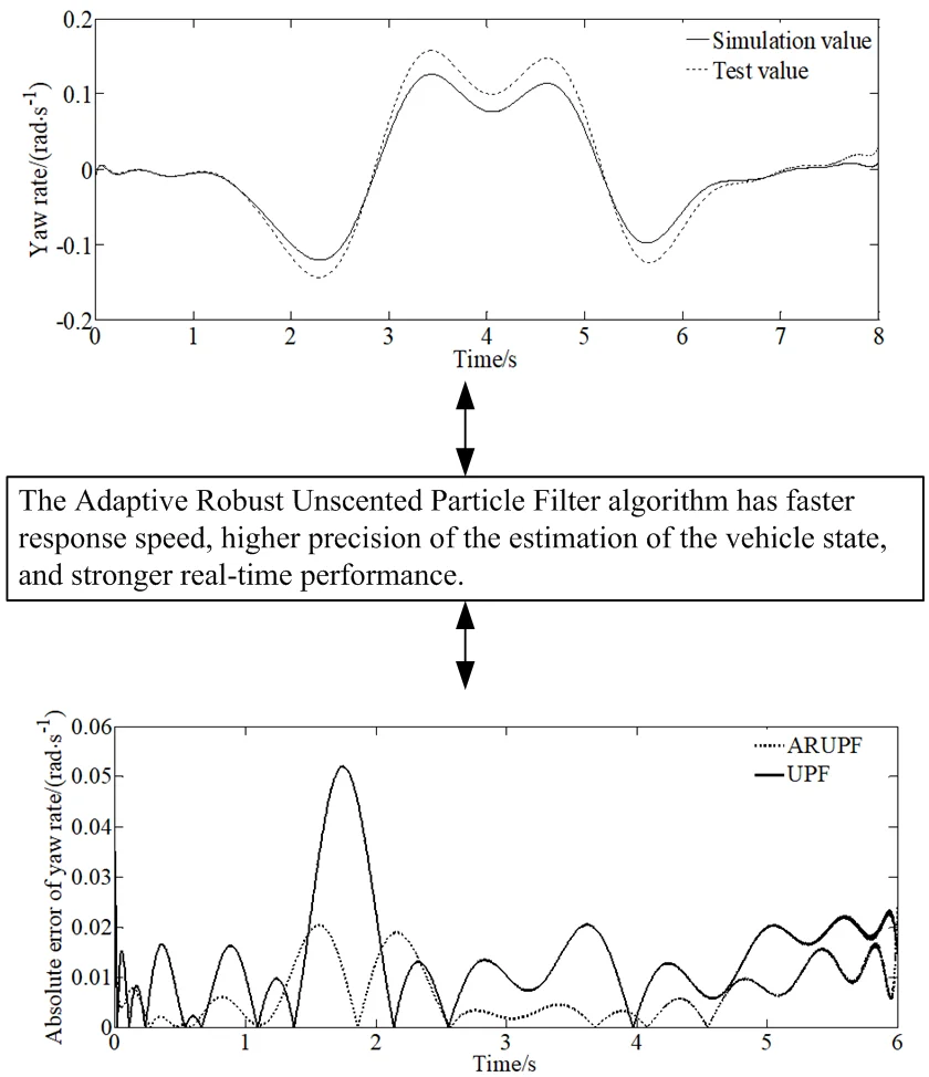
In order to solve the problem that the measured values of key state parameters such as the lateral velocity and yaw rate of the vehicle are easily interfered by random errors, a filter estimation method of vehicle state is proposed based on the principle of robust filtering and the unscented particle filter algorithm. Based on the establishment of a 3-DOF non-linear dynamic model and the Dugoff tire model of the vehicle, the adaptive robust unscented particle filter(ARUPF) is used to filter and estimate the parameters of the vehicle state, and to realize the longitudinal and lateral speed as well as the yaw rate of the vehicle during the driving process. The simulation and the real vehicle test results show that based on the adaptive robust unscented particle filter algorithm, the vehicle driving state estimation can be realized, the measurement parameters can be effectively filtered, and the estimation accuracy is high.
Highlights
- The adaptive robust unscented particle filter algorithm can realize the vehicle driving state estimation.
- The adaptive robust unscented particle filter algorithm can effectively filter the measurement parameters.
- The adaptive robust unscented particle filter algorithm has higher estimation accuracy.
1. Introduction
When analyzing the active safety of a vehicle, it is particularly important to obtain the state parameters during the driving process of the vehicle. The algorithms used to estimate the key state parameters of automobiles mainly include Kalman filter algorithm, particle filter algorithm, sliding mode observer algorithm, robust observer algorithm and Romberg observer algorithm. The sliding mode observer algorithm depends on the accuracy and performance of the sensor, otherwise it is prone to chattering. The robust observer algorithm is prone to underestimation bias in some cases, which causes the algorithm to diverge. The calculation process of the Romberg observer algorithm is complex, and it is difficult to meet the real-time requirements of the vehicle estimation algorithm.
A vehicle is a strong nonlinear system, but the Kalman filter can only process linear systems. Based on the standard Kalman filter algorithm, the Extended Kalman Filter (EKF) and Unscented Kalman Filter (UKF) are developed to handle nonlinear systems. The extended Kalman filter algorithm linearizes the nonlinear system by performing Taylor expansion of the mathematical model of the nonlinear system at the optimal point, and solving the Jacobian matrix of the nonlinear function. When this algorithm is used to linearize the nonlinear system, only the first-order system is retained, and the second-order or higher-order components are discarded, so there is a certain estimation bias. At the same time, when the estimated target system has strong nonlinearity, its calculation amount is too large and the Jacobian matrix is complicated to solve, so the divergence is easy to occur. For each sigma point obtained, its mean and variance are ensured the same as the original data, and brought into the nonlinear system for unscented transformation making it close to Gaussian distribution through weighted summation of samples. Based on the characteristics of Gaussian distribution, the algorithm can be accurate to the third-order mean and covariance, and the operation is simple, and the obtained system is stable.
The problem of vehicle state estimation has been widely studied. A brief review is presented in what follows.
Lenzo et al.[1] proposed an Extended Kalman Filter (EKF) method to estimate the vehicle states as well as tyre-road coefficient of friction. Li et al. [2] proposed a new situation-sensitive method to improve the vehicle detection at nighttime. In order to estimate vehicle states and parameter with high precision, Zhu et al. [3] presented a modified particle filter. Wang et al. [4] proposed a novel adaptive fault-tolerant extended Kalman filter to estimate vehicle state in case of partial loss of sensor data. In order to improve the driving dynamics and the driving safety, Henning et al.[5] presented an integrated lateral dynamics control concept for a over-actuated vehicle. Zhao et al. [6] presented a state estimation method to enable fully autonomous flight in outdoor environments. Alatorre et al. [7] proposed an algorithm that merges the concepts of least squares method and sliding mode observer for the estimation of the vehicle mass. Heidfeld et al. [8] proposed an Unscented KALMAN Filter (UKF) for simultaneous state and parameter estimation. Badini et al. [9] presented a simple parameter independent speed estimation algorithm for vector-controlled permanent magnet synchronous motor (PMSM) drive. Kulikov et al. [10] resolved the lack of square-root implementations by means of hyperbolic QR transforms applied for yielding J-orthogonal square roots. Malikov [11] solved the problem of differential equations with periodic using the quadratic Lyapunov function. Takikawa1 et al. [12] used a global navigation satellite system (GNSS) Doppler for accurate vehicular trajectory estimation. Gao et al. [13, 14] presented a new methodology of distributed state fusion for multisensory nonlinear systems by using the sparse-grid quadrature filter.
In the literatures proposed above, some researchers did not implement the algorithms in onboard real-time systems. And some researchers missed the diverse traffic conditions in daytime and nighttime when estimating states of the vehicle. At the same time, more vehicle parameters including the yaw inertia of the vehicle hadn’t been estimated in a lot of literatures. And the estimation error covariance as well as the closed-loop operation of the state estimator with a driving dynamic hadn’t been investigated. For some researchers, the usability of the proposed model should be improved.
In the current research, most of the observation noise covariance matrix is set to a fixed value. However, in the actual driving process of the vehicle, the process noise and observation noise are randomly generated. The unscented particle filter (UPF) algorithm uses the unscented Kalman filter method to generate the proposal density function, so that the prior probability peak value and the likelihood function peak value have good agreement reducing particle degradation. However, the accuracy is affected by the uncertainty of the system noise. And the lack of an adaptive adjustment mechanism makes it impossible to adjust the filter gain and related parameters in real time. In order to better estimate the state parameters of the vehicle in real-time and effectively, the adaptive robust unscented particle filter (ARUPF) method, which can adjust filter parameters in real time and has better adaptability to interference noise is proposed.
The ARUPF algorithm absorbs the advantages of robust estimation, robust adaptive filtering and particle filtering fully. It combines robust estimation principle and the UPF algorithm through equivalent weight function and adaptive factor. The state model information and measurement model information can be controlled by selecting appropriate weight function and adaptive factor, suppressing the influence of abnormal interference. The ARUPF algorithm overcomes the shortcomings of using only a single filtering algorithm. The algorithm uses the important density function selected from the three important steps of UT transformation, equivalent weight and adaptive factor adjustment to perform importance sampling, reducing the degree of particle degradation, and having high filtering accuracy.
2. Mathematical model of vehicle dynamics
2.1. 3-DOF vehicle model
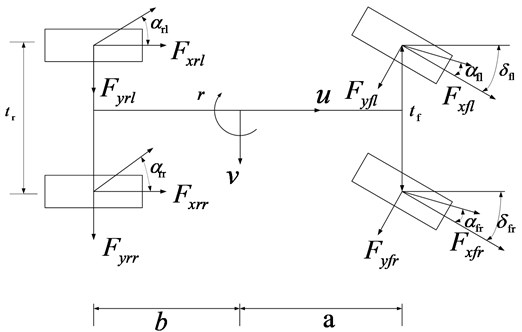
The vehicle state estimation model is established based on a 3-DOF vehicle model. The 3-DOF vehicle model is shown in Fig. 1. is the vehicle coordinate system, and the origin of the vehicle coordinate system coincides with the center of mass of the vehicle.
Fig. 13-DOF vehicle model
The paper adopts a simplified estimation model, and establishes a nonlinear 3-DOF vehicle model including longitudinal and lateral as well as yaw motion. And it is assumed that:
(1) The center of mass of the vehicle model coincides with the origin of the vehicle coordinate system;
(2) The suspension has no effect on the vertical movement of the vehicle;
(3) The vehicle has no degree of freedom in the pitch and roll directions;
(4) The impact of the longitudinal rolling resistance is ignored for the state parameter estimation.
In Fig. 1, and are the distances of front and rear axles from the center of gravity respectively; and are the tracks of the front and rear wheels respectively; are the side slip angles of the left and right front wheels; are the side slip angles of the left and right rear wheels; are the longitudinal forces of the left front, right front, left rear, and right rear wheels; are the lateral forces of the left front, right front, left rear, and right rear wheels; are the wheel angles of the left and right front wheels.
The dynamic equation of the 3-DOF vehicle model is as follows:
where, and are the longitudinal and the lateral speed; is the yaw rate; and the longitudinal and lateral acceleration; is the yaw moment; is the moment of inertia around the z axis of the vehicle.
The side slip angle of the center of mass is:
According to the kinetic equation, the calculation formulas for other parameters are as follows:
where, is the vehicle mass; is the height of the center of mass; is the rolling radius of the wheels; is the wheelbase; is the center speed of the left and right front wheels; is the center speed of the left and right rear wheels; is the vertical load of the left and right front wheels; is the vertical load of the left and right rear wheels.
2.2. Tire model
The expression of the Dugoff tire model is relatively simple, with fewer unknown parameters, and can accurately describe the nonlinear characteristics of tire friction. Therefore, the tire model selected in this article is the Dugoff tire model [15]:
where and are the longitudinal and cornering stiffness of the tires respectively; is the longitudinal slip ratio; is the slip angle of the tire; indicates , , and ; is the road friction coefficient; when , the wheel is in the linear state area; when , the wheel is in the non-linear state region.
2.3. Nonlinear vehicle system containing noise
The state vector of the nonlinear vehicle system is set as , the system input is , and the observation vector is .
3. The ARUPF Algorithm
The traditional particle filter algorithm has the defect of particle degradation in the iterative process, resulting in waste of computing resources and low accuracy of estimation results. In order to solve the above problems, the filtering algorithm is often optimized by increasing the number of particles, re-sampling, and selecting a reasonable proposal density function. Increasing the number of particles can effectively alleviate the particle degradation, but it increases the computational workload of the system. The re-sampling method can increase the diversity of particles and avoid particle degradation. The adaptive robust unscented particle filter algorithm uses the unscented transformation algorithm to calculate the mean and covariance of each particle and establish a reasonable proposal density function combining the robust filter estimation algorithm to automatically adjust the gain matrix and system variance making the distribution of sample points fit better with the maximum likelihood function. Unscented particle filter algorithm is easy to implement in engineering and can effectively reduce the workload of the system. The specific methods are as follows:
1) Initialization, 0.
Drawing initial state particles from the prior distribution:
where and are the mathematical expectation and variance of the initial particle respectively, and are the mathematical expectation and variance of the initial Sigma point, respectively; and are the covariance matrix and the observation covariance matrix of the system respectively.
2) Importance sampling.
Calculating the mean and variance using the unscented Kalman algorithm.
(1) Extracting the set of Sigma points:
where and are the mathematical expectation and variance of the extracted particles respectively; and are the state dimension and scaling factor respectively.
(2) One-step prediction for the Sigma point set:
where , and are state value, mathematical expectation and variance of the Sigma particle after one-step prediction respectively; and are the observed value and the observed mean value obtained by inputting the observation equation for the Sigma point after one-step prediction respectively; and are the calculation weights of the mean and the covariance corresponding to Sigma respectively.
(3) Integrating the observation data to update the mean, Kalman gain and covariance of the Sigma point set:
where and are the observed covariance and system variance obtained by weighted calculation respectively; , and are the system gain matrix, state value and variance after state update respectively.
3) ARUPF algorithm.
The ARUPF algorithm is based on robust estimation filtering theory, which controls the abnormal situation of the observed value of the dynamic model, and constructs an adaptive factor to control the error of the dynamic model. If is set as the weight matrix of the state matrix , the equivalent weight matrix is . The principle for using the IGG (Institute of Geodesy & Geophysics) method to generate the equivalent weight function is as follows:
where is the detect residual values for sensors; the value range of the adjustment factor are and .
It is set that the sensor perception matrix is . The system state vector is updated according to the weight matrix obtaining the system state solution vector of the adaptive robust Kalman filter:
where is the adaptive factor; is the matrix trace operator; the ranges of the regulators and are , .
In the above formula, the weight matrix is obtained by judging the residual error; the adaptive factor is obtained by the difference operation between the state estimated value and the predicted value. The two parameters are used to adjust the Kalman gain, the sampled particle mean and the particle weight at the same time and update the particle and normalize weights:
where is the Kalman gain computed by the robustness algorithm; is the State sample mean; is the sample variance; is the updated particle weight value.
Using the resampling algorithm, the particle set is eliminated and copied based on the normalized weight, and the weight is reset to the new particle. When the prediction model has excessive abnormal interference, the adaptive factor is decreased, which can weaken the influence of the interference. When there is a large disturbance in the observation model, the abnormal influence caused by the disturbance can be reduced by adjusting the weight matrix . The adaptive robust unscented particle filter algorithm can effectively solve the problem of gross error and abnormal state of the system observation, and establish a reasonable particle filter which effectively solves the problem of particle degradation.
4. Numerical simulations and experimental verification
4.1. Numerical simulations
A Volkswagen vehicle is verified by a simulation test on the virtual prototype software ADAMS. And the real vehicle used for test is the same with the virtual vehicle model in Adams. That is to say, the parameters of the vehicle dynamics model in ADAMS are the same as our test vehicle shown in Table 1.
ADAMS/Car adopts a top-down modeling sequence. That is to say, the vehicle model and the system assembly model are built on the basis of each subsystem model. And each subsystem model needs to be established by templates, so the establishment of each template is the key steps to establish the vehicle model. The template establishment process is as follows:
(1) Simplification of the physical model: According to the relative motion relationship between the various parts of the subsystem, defining the “Topological Structure” of the parts, integrating the parts, and defining the parts without motion relationship as a “Gene-ralPart”.
(2) Determining “Hard Point”: The hard point is the geometric positioning point at the key connection point of the part, and the determination of the hard point is to determine the geometric coordinates of the key point of the part. To determine the hard point is to determine the geometric coordinates of the key points of the part in the subsystem coordinate system, and the hard point can be modified in the vehicle model and template state.
Table 1Simulation parameters
Parameter | Value |
(kg) | 1558 |
(kg∙m2) | 2538 |
(m) | 1.48 |
(m) | 1.08 |
(m) | 0.432 |
(m) | 1.51 |
(m) | 1.55 |
(m) | 0.32 |
(3) Determining the parameters of the part: Calculating or measuring the mass of the integrated part, the position of the center of mass, and the moment of inertia around the three axes of the center of mass coordinate system. It should be noted that the directions of the three coordinate axes of the center of mass coordinate system must be parallel to the directions of the three axes of the system coordinate system.
(4) Creating the “Geometry” of the part: Building the geometric model of the part on the basis of the hard point. Since the dynamic parameters of the part have been determined, the shape of the geometric model has no influence on the dynamic simulation results. But in the kinematic analysis, the outer contour of the part is directly related to the motion check of the part. And the intuitiveness of the model is considered. And considering the intuitiveness of the model, the geometry of the part should be as close to the actual structure as possible.
(5) Defining “Constrain”: Defining the type of constraint according to the motion relationship between parts. The components are connected by constraints to form the subsystem structure model. Defining constraints is the key to correct modeling and is directly related to the rationality of the degrees of freedom of the system.
(6) Defining “Mount”: Defining assembly commands at the connections between subsystems and subsystems or external models.
(7) Defining “Subsystem”: Transferring the model built in Template to the standard mode and defining each subsystem model preparing for assembling the vehicle model.
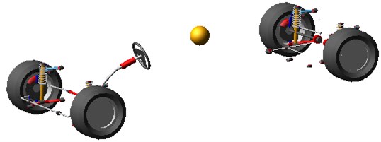
Fig. 2Vehicle model in ADAMS
(8) Defining “Assembly”: In the standard mode, each subsystem is assembled into a complete vehicle model. So that the establishment process of the physical model is completed in the ADAMS/Car module. By adding attribute files, the simulation analysis of the vehicle under different working conditions can be carried out to obtain the required results.
The vehicle model can be obtained as shown in Fig. 2.
4.1.1. Sine delay test
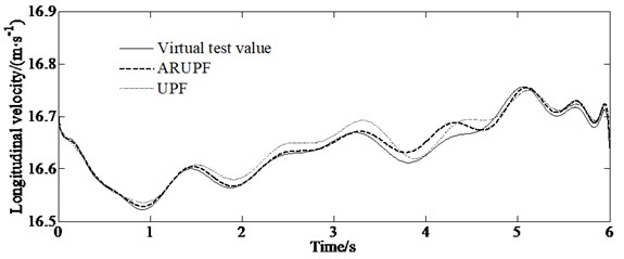
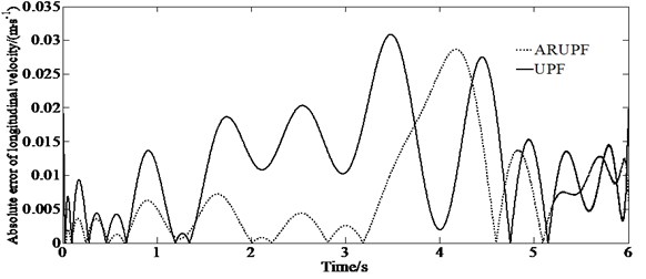
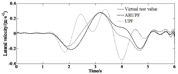
The sine delay test is carried out on a dry, flat and clean cement test site. The test vehicle drives at a constant speed of (80±2) km/h. The virtual test value, the experimental measurements, the estimation results of the ARUPF and the UPF algorithm are shown in Fig. 3. The results show that the ARUPF algorithm achieves better estimation results for the longitudinal velocity and the yaw rate, while the estimation results of the UPF algorithm have a certain amplitude fluctuation in the steering wheel holding stage. For the lateral velocity, the ARUPF There is a small deviation between the estimated value of the ARUPF algorithm and the virtual test value at the peak. But the overall estimated result meets the engineering needs. And the estimated result of the UPF algorithm is different from the virtual test value during the steering wheel rotation process. There is a certain magnitude of fluctuation in the steering wheel holding process.
Fig. 3Comparison of the state variables found with the different algorithms (ARUPF and UPF) for a sine delay test road
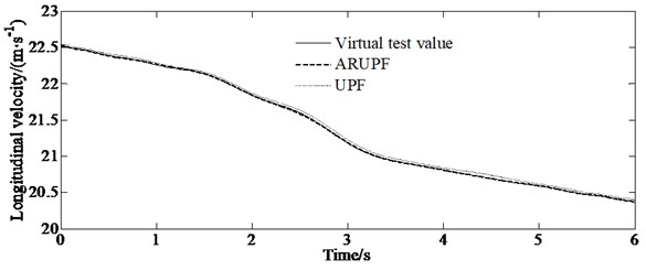
a) Longitudinal velocity
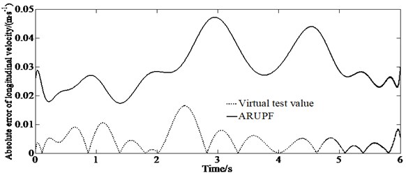
b) Absolute error of longitudinal velocity
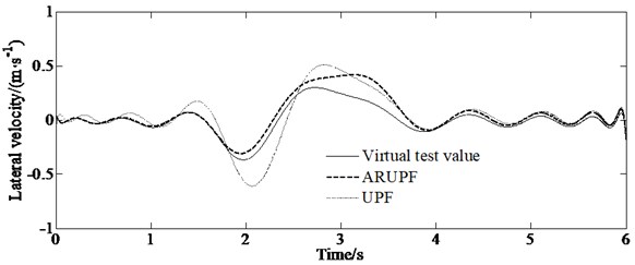
c) Lateral velocity
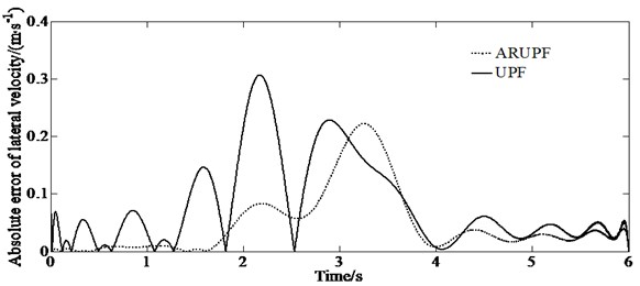
d) Absolute error of lateral velocity
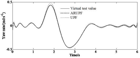
e) Yaw rate
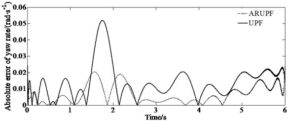
f) Absolute error of yaw rate
The ARUPF algorithm has the advantages of robust estimation and unscented particle filtering. After comprehensively selecting the important density function by using unscented transformation, equivalent weight function and adaptive adjustment factor, the importance sampling of particles is carried out. And the sensor perception vector is used reasonably. It effectively suppresses the pollution problem of state parameters and the abnormal disturbance of sensor perception values, reducing the degree of particle degradation in the process of vehicle state estimation and overcoming the shortcomings of a single filtering algorithm. The reasons for this error are as follows: since the mathematical model ignores the suspension characteristics and tire rolling resistance, the tire slip angle and the lateral load transfer of the sprung mass have a certain relationship with the tire slip angle and tire vertical load in ADAMS. However, the observer can effectively estimate the vehicle state such as the longitudinal and lateral velocity, as well as the yaw rate, etc.
4.1.2. Double lane change test
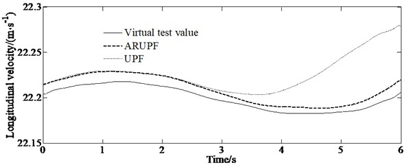
A double lane change test is carried out on a dry, flat and clean cement test site. The test speed is 60 km/h. The test driver make the vehicle pass through the double lane change channel without touching the stakes. The virtual test value, the experimental measurements, the estimation results of the ARUPF and the UPF algorithm are shown in Fig. 4.
Fig. 4Comparison of the state variables found with the different algorithms (ARUPF and UPF) for a double lane change test road
a) Longitudinal velocity
b) Absolute error of longitudinal velocity
c) Lateral velocity
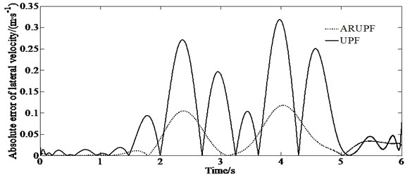
d) Absolute error of lateral velocity
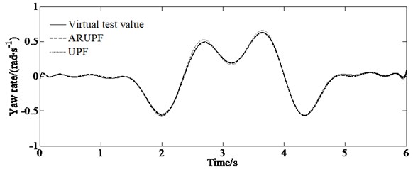
e) Yaw rate
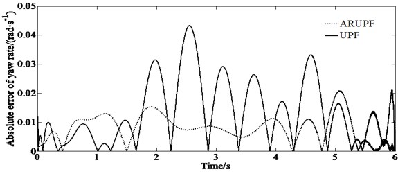
f) Absolute error of yaw rate
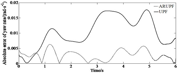
This test condition is used to verify the accuracy of the algorithm for estimating the longitudinal and lateral velocity as well as the yaw rate of the vehicle when the vehicle states change rapidly. The results show that the ARUPF algorithm has achieved good results in the estimation of the longitudinal velocity and the yaw rate. But the UPF algorithm has a small fluctuation in the estimation of the longitudinal velocity and the yaw rate. For the lateral velocity, there is a certain magnitude of deviation between the estimated results of the ARUPF algorithm and the virtual test value during the steering wheel rotation, while the estimated results of the UPF algorithm have large fluctuations.
The average absolute error (MAE) and root mean square error (RMSE) are given to verify the estimation accuracy of the proposed algorithm.
Table 2The MAE and RMSE indicators of the two algorithms
Evaluation index | State value | UPF | ARUPF |
MAE | (m/s) | 0.316 | 0.140 |
(m/s) | 0.181 | 0.0475 | |
(rad/s) | 0.316 | 0.0180 | |
RMSE | (m/s) | 0.345 | 0.141 |
(m/s) | 0.243 | 0.0522 | |
(rad/s) | 0.411 | 0.0221 |
From Table 2, it can be seen more intuitively that the estimation accuracy of the ARUPF algorithm is significantly higher than the UPF method.
The ARUPF algorithm has the advantages of robust estimation and unscented particle filtering. After comprehensively selecting the important density function by using unscented transformation, equivalent weight function and adaptive adjustment factor, the importance sampling of particles is carried out. And the sensor perception vector is used reasonably. It effectively suppresses the pollution problem of state parameters and the abnormal disturbance of sensor perception values, reducing the degree of particle degradation in the process of vehicle state estimation and overcoming the shortcomings of a single filtering algorithm. The reasons for this error are as follows: since the mathematical model ignores the suspension characteristics and tire rolling resistance, the tire slip angle and the lateral load transfer of the sprung mass have a certain relationship with the tire slip angle and tire vertical load in ADAMS. However, the observer can effectively estimate the vehicle state such as the longitudinal and lateral velocity, as well as the yaw rate, etc.
4.1.3. Slop input test
A slope input test is carried out on a dry, flat and clean cement test site, the vehicle speed is maintained at 80 km/h. The virtual test value, the experimental measurements, the estimation results of the ARUPF and the UPF algorithm are shown in Fig. 5. The test can make the vehicle gradually enter the limit working condition as the steering wheel angle increases, and the tire gradually transitions from the linear working area to the nonlinear working area, which leads to the increase of the error of the model of the vehicle.
Fig. 5Comparison of the state variables found with the different algorithms (ARUPF and UPF) for a slop input test road
a) Longitudinal velocity
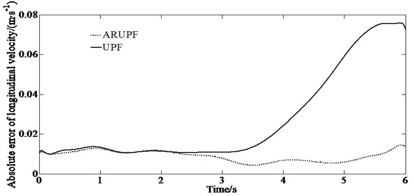
b) Absolute error of longitudinal velocity
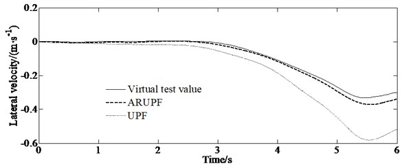
c) Lateral velocity
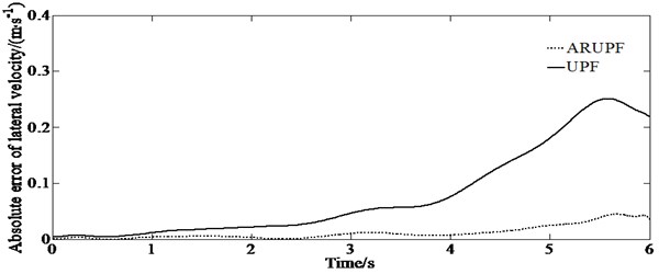
d) Absolute error of lateral velocity
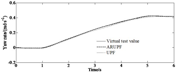
e) Yaw rate
f) Absolute error of yaw rate
It can be seen from Fig. 5 that when the system noise increases, the estimation deviation of the UPF algorithm for the longitudinal lateral speed gradually increases. For the estimation of yaw rate, both the UPF algorithm and the ARUPF algorithm maintain a high estimation accuracy.
The ARUPF algorithm has the advantages of robust estimation and unscented particle filtering. After comprehensively selecting the important density function by using unscented transformation, equivalent weight function and adaptive adjustment factor, the importance sampling of particles is carried out. And the sensor perception vector is used reasonably. It effectively suppresses the pollution problem of state parameters and the abnormal disturbance of sensor perception values, reducing the degree of particle degradation in the process of vehicle state estimation and overcoming the shortcomings of a single filtering algorithm. The reasons for this error are as follows: since the mathematical model ignores the suspension characteristics and tire rolling resistance, the tire slip angle and the lateral load transfer of the sprung mass have a certain relationship with the tire slip angle and tire vertical load in ADAMS. However, the observer can effectively estimate the vehicle state such as the longitudinal and lateral velocity, as well as the yaw rate, etc.
4.2. Experimental verification
According to ISO/TR3888-2004, the real vehicle test on double lane change road is carried out. And the test speed is set as 80 km/h (±3 km/h). A gyroscope is installed on the vehicle to collect the yaw rate and lateral acceleration of the vehicle in real time. The non-contact speed sensor is used to measure the longitudinal and lateral speed of the vehicle. In addition, the steering wheel angle tester is used to measure the steering wheel angle. Fig. 6 is the comparison between the estimated value of ARUPF method of three state variables and the real vehicle test value.
Fig. 6Comparison of the estimated and test values
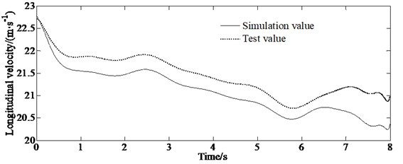
a) Longitudinal velocity
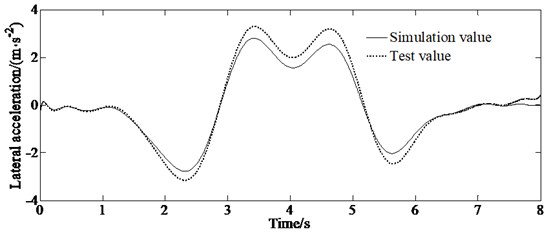
b) Lateral acceleration
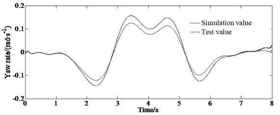
c) Yaw rate
From Fig. 6, it can be seen that although there is a certain error, the estimated value is basically consistent with the experimental value in trend. There is a large difference between the experimental value and the estimated value of the longitudinal velocity, because the estimation of the longitudinal velocity in the model is affected by many parameters such as longitudinal acceleration, lateral velocity and yaw rate. And the tire model used in this paper still has some deviation when simulating the mechanical characteristics of real vehicle tire. In addition, the measurement error and installation position of the sensor are also important reasons for the deviation between the estimated and the test value.
5. Conclusions
Based on the Dugoff tire model, a 3-DOF dynamic model of the vehicle with front wheel steering is established to estimate the longitudinal and lateral speed and the yaw rate of the vehicle. The equivalent weight function is generated by using the IGG method. By adaptively adjusting the weight matrix, the random error caused by nonlinear factors in the process of vehicle sensor detection can be effectively suppressed. And the influence of data distortion caused by interference can be reduced, and the accuracy of vehicle state estimation is improved. Based on the principle of adaptive robust filter and unscented particle filter algorithm, a new state estimation method of vehicle is proposed. The ARUPF method has the advantages of good noise filtering effect and high precision. A simulation platform is used to simulate, analyze and verify the estimation effect of the proposed algorithm. The simulation results show that the vehicle state estimation based on the ARUPF algorithm has the characteristics of high precision, strong anti-interference ability and good stability. It has the advantages of low cost, easy engineering implementation providing a new idea for vehicle state estimation.
References
-
B. Lenzo, G. Ottomano, S. Strano, M. Terzo, and C. Tordela, “A physical-based observer for vehicle state estimation and road condition monitoring,” in IOP Conference Series: Materials Science and Engineering, Vol. 922, No. 1, p. 012005, Sep. 2020, https://doi.org/10.1088/1757-899x/922/1/012005
-
J. L. Li et al., “Domain adaptation from daytime to nighttime: A situation-sensitive vehicle detection and traffic flow parameter estimation framework,” Transportation Research Part C, Vol. 124, pp. 1–19, 2021, https://doi.org/10.1016/j.trc.2020.10294
-
J. Zhu, Z. Wang, L. Zhang, and W. Zhang, “State and parameter estimation based on a modified particle filter for an in-wheel-motor-drive electric vehicle,” Mechanism and Machine Theory, Vol. 133, pp. 606–624, Mar. 2019, https://doi.org/10.1016/j.mechmachtheory.2018.12.008
-
Y. Wang, L. Xu, F. Zhang, H. Dong, Y. Liu, and G. Yin, “An adaptive fault-tolerant EKF for vehicle state estimation with partial missing measurements,” IEEE/ASME Transactions on Mechatronics, Vol. 26, No. 3, pp. 1318–1327, Jun. 2021, https://doi.org/10.1109/tmech.2021.3065210
-
K.-U. Henning, S. Speidel, F. Gottmann, and O. Sawodny, “Integrated lateral dynamics control concept for over-actuated vehicles with state and parameter estimation and experimental validation,” Control Engineering Practice, Vol. 107, p. 104704, Feb. 2021, https://doi.org/10.1016/j.conengprac.2020.104704
-
M. Zhao et al., “Versatile multilinked aerial robot with tilted propellers: design, modeling, control, and state estimation for autonomous flight and manipulation,” Journal of Field Robotics, Vol. 38, No. 7, pp. 933–966, Oct. 2021, https://doi.org/10.1002/rob.22019
-
A. Alatorre, E. S. Espinoza, B. Sánchez, P. Ordaz, F. Muñoz, and L. R. García Carrillo, “Parameter estimation and control of an unmanned aircraft‐based transportation system for variable‐mass payloads,” Asian Journal of Control, Vol. 23, No. 5, pp. 2112–2128, Sep. 2021, https://doi.org/10.1002/asjc.2565
-
H. Heidfeld and M. Schünemann, “Optimization-based tuning of a hybrid UKF state estimator with tire model adaption for an all wheel drive electric vehicle,” Energies, Vol. 14, No. 5, p. 1396, Mar. 2021, https://doi.org/10.3390/en14051396
-
S. S. Badini and V. Verma, “Parameter independent speed estimation technique for PMSM drive in electric vehicle,” International Transactions on Electrical Energy Systems, Vol. 31, No. 11, pp. 13071–13090, Nov. 2021, https://doi.org/10.1002/2050-7038.13071
-
G. Y. Kulikov and M. V. Kulikova, “Square-root high-degree cubature Kalman filters for state estimation in nonlinear continuous-discrete stochastic systems,” European Journal of Control, Vol. 59, pp. 58–68, May 2021, https://doi.org/10.1016/j.ejcon.2021.02.002
-
A. I. Malikov, “State estimation and control for linear aperiodic impulsive systems with uncertain disturbances,” Russian Mathematics, Vol. 65, No. 6, pp. 36–46, Jun. 2021, https://doi.org/10.3103/s1066369x21060050
-
K. Takikawa, Y. Atsumi, A. Takanose, and J. Meguro, “Vehicular trajectory estimation utilizing slip angle based on GNSS Doppler/IMU,” Robomech Journal, Vol. 8, No. 1, pp. 1–11, Dec. 2021, https://doi.org/10.1186/s40648-021-00195-4
-
B. Gao, G. Hu, Y. Zhong, and X. Zhu, “Distributed state fusion using sparse-grid quadrature filter with application to INS/CNS/GNSS integration,” IEEE Sensors Journal, Vol. 22, No. 4, pp. 3430–3441, Feb. 2022, https://doi.org/10.1109/jsen.2021.3139641
-
B. Gao, G. Hu, Y. Zhong, and X. Zhu, “Cubature rule-based distributed optimal fusion with identification and prediction of kinematic model error for integrated UAV navigation,” Aerospace Science and Technology, Vol. 109, p. 106447, Feb. 2021, https://doi.org/10.1016/j.ast.2020.106447
-
R. He, E. Jimenez, D. Savitski, C. Sandu, and V. Ivanov, “Investigating the parameterization of dugoff tire model using experimental tire-ice data,” SAE International Journal of Passenger Cars – Mechanical Systems, Vol. 10, No. 1, pp. 83–92, Sep. 2016, https://doi.org/10.4271/2016-01-8039
Cited by
About this article

This research was supported by the Science and Technology Program Foundation of Weifang under Grant 2015GX007. And also, this research was financially supported by the Open Research Fund from the State Key Laboratory of Rolling and Automation, Northeastern University, under Grant 2021RALKFKT008. The first author gratefully acknowledges the support agency.
The datasets generated during and/or analyzed during the current study are available from the corresponding author on reasonable request.
The authors declare that they have no conflict of interest.
