Abstract
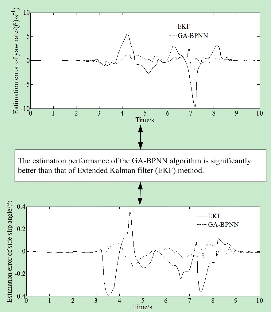
A multi-machine-learning improved adaptive Kalman filtering method is proposed to address the problem of handling abnormal data encountered in the vehicle state estimation. Firstly, the unscented Kalman filter (UKF) algorithm is improved by introducing a BP neural network improved by the genetic algorithm (GA-BPNN) to regulate and correct the global error of the UKF method. Then, the anti-outlier technique is applied to fully eliminate isolated and speckled outliers in the measurement, achieving further improvement on GA-BPNN-UKF and significantly improving the robustness of the filtering process. Finally, a simulation is applied to verify the effectiveness of the proposed new algorithm, and then its results are analyzed to obtain a firm substantiation of its effectiveness for further practical applications. The simulation results indicate that the estimation performance of the GA-BPNN algorithm is significantly better than that of Extended Kalman filter (EKF) method.
Highlights
- The anti-outlier technique is applied to fully eliminate isolated and speckled outliers in the measurement, achieving further improvement on GA-BPNN-UKF and significantly improving the robustness of the filtering process.
- The estimation performance of the GA-BPNN algorithm is significantly better than that of Extended Kalman filter (EKF) method.
- The algorithm presented in the paper has a higher solution efficiency under the same calculation accuracy.
1. Introduction
Being the main kind of transport in modern society, vehicles have promoted the development and progress of society. However, at the same time, with the rapid rise of automotive technology and the increase in vehicle ownership, they brought significant traffic safety hazards.
In recent years, autonomous driving technology developed rapidly, and its safety was widely concerned by society. As autonomous driving technology leaves the laboratory and enters society, it will face more complex traffic conditions. In order to ensure the safety of the vehicle itself, it needs to accurately perceive the environment it faces and make reasonable decisions.
At present, many high-precision sensors cannot be widely used in all vehicles due to their high cost. In addition, sometimes it is difficult to measure directly some key state parameters. Therefore, it is necessary to use some relatively inexpensive sensors to obtain a portion of state information firstly, and use this information to estimate the key vehicle states that are not suitable for direct measurement, effectively ensuring the safety and autonomous driving of vehicles.
The implementation of automotive active control systems and intelligent driving systems is based on obtaining the basic plane motion state of the vehicle, that is, obtaining longitudinal and lateral velocities, and yaw rate. Generally speaking, this information can be directly obtained from sensors. However, due to the limitations of sensor accuracy and cost, as well as the difficulty in determining the distribution characteristics of measurement noise, it is impossible to find effective and applicable sensors for direct measurement, or the measurement accuracy is not optimal for some state information [1].
A reasonable method is to use cheap sensor information combined with state estimation algorithms for soft measurement. The traditional motion state estimation algorithm mainly adopts the model-based method, using kinematic and dynamic models to describe the relationship between longitudinal and lateral velocities, yaw rate and other vehicle parameters and states. Algorithms such as Kalman Filter (KF) unite a series of noise measurement results with estimation results based on linear models, which makes them suitable for conventional driving conditions. The Extended Kalman Filter (EKF) adopts a nonlinear vehicle model with a better estimation accuracy than KF. The unscented Kalman filter (UKF) utilizes the UT transform to avoid linearization processing and has higher estimation accuracy.
The problem of vehicle state estimation has been widely studied. A brief review is presented in what follows.
Tian et al. proposed the parameter estimation method based on multi-dimensional information fusion [2]. And also, a comprehensive evaluation of wheel dynamics state was also realized by this information fusion. Yu et al. introduced a vehicle mass estimation method based on fusion of the machine learning and vehicle dynamic model [3]. Cai et al. demonstrated and opened for academic research six sets of electric vehicle data collected during experiments on a low-adhesion road [4]. Amin et al. introduced a review on the vehicle-trailer state and parameter estimation including trailer snaking, jack-knifing, and roll-over [5]. Xiang et al. proposed a sideslip recognition model that used the perception information of driverless vehicles to assess the sideslip driving status of the surrounding vehicles [6]. Xu et al. proposed a hierarchical estimation model considering the current rate to solve this problem [7]. Xue et al. developed a novel robust unscented M-estimation-based filter (RUMF) for the state estimation of a vehicle with unknown driver steering torque [8]. Zhang et al. proposed a state estimation method based on the enhanced adaptive unscented Kalman filter (EAUKF) to solve vehicle estimation under unknown noise conditions [9]. Qin et al. proposed a lateral and longitudinal dynamics control framework of autonomous vehicles considering the multi-parameter joint estimation in order to improve the trajectory tracking accuracy and vehicle lateral stability [10]. Jasmina et al. proposed an innovative way for the mode mixing involving the state-vectors for the models with different size [11]. Muhammed Hafiz et al. proposed a method aiming to determine a queue and delay for a signalized intersection approach using the data obtained from RFID sensors [12]. Zhang et al. presented a joint state-of-charge (SOC) and state-of-available-power (SOAP) estimation method based on the online battery model parameter identification [13]. Jiang et al. investigated a novel cell-to-pack state estimation extension method based on a multilayer difference model (MDM) to address the difficulty of state estimation by cell inconsistency and to realize the joint estimation of the state-of-charge (SOC) and capacity for series-connected battery packs [14]. Wael proposed a real-Time Monte Carlo Localization (RT_MCL) method for autonomous cars [15]. Wang et al. proposed a method of tire road friction coefficient estimation with review and research perspectives [16]. Duc et al. introduced an anti-slip controller for a quarter vehicle traction control system [17]. Karnika et al. proposed a method aiming at establishing an alternative approach to dynamic modeling and robust control with online estimation of slip parameters [18]. This approach provides for modifying the kinematic model such that it was capable to accommodate slip-disturbance inputs. Wang et al. proposed a novel vehicle detection and tracking method for small target vehicles to achieve high detection and tracking accuracy based on the attention mechanism [19]. Gao et al. proposed a vehicle localization system based on vehicle chassis sensors considering vehicle lateral velocity to improve the accuracy of vehicle stand-alone localization in highly dynamic driving conditions during Global Navigation Satellites Systems outages [20]. Ding et al. proposed a driving strategy for network and autonomous vehicles that considered multiple preceding vehicles, including human-driven vehicles [21].
To sum up, the above literature used a variety of methods to identify effectively the states and parameters of vehicles, but some of the applied methods can hardly achieve the effective estimation for systems with many parameters and strong nonlinearity. In the actual test system, due to the limitations of test means, test environment and other factors, the measurement may include outlier in addition to noise. This outlier will reduce the performance of the data processing algorithm, and in serious cases, it will lead to algorithm divergence, making the estimation error far greater than the impact of the measurement error.
In response to the above shortcomings, this article proposes a high-precision Kalman filtering algorithm with fault-tolerant performance based on multiple optimization algorithms. On the basis of the unscented Kalman filter, an anti-outlier algorithm is introduced to eliminate effectively isolated and spotted outliers that appear during the measurement process. At the same time, a BP neural network based on the improved genetic algorithm is introduced to improve effectively its filtering accuracy.
2. Mathematical model of vehicle state estimation problem
2.1. 3-DOF vehicle model
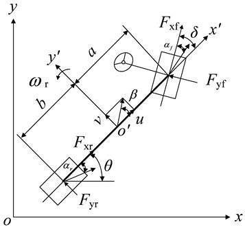
Based on reasonable assumptions and simplification, this paper obtains a nonlinear vehicle dynamics model including the longitudinal and lateral yaw motion of the vehicle body as shown in Fig. 1:
where is the vehicle mass; is the moment of inertia around the axis; , and are the yaw, yaw rate and yaw angular acceleration of the vehicle respectively; and are the distances of front and rear axles from the center of gravity; and are the lateral forces of front and rear tires; is the longitudinal force of tire; and are the speed in vehicle coordinate system; and are the accelerations in the vehicle coordinate system.
The motion of a vehicle in the global coordinate system can be represented as:
where and are velocities of the lateral and longitudinal motions of vehicles in the global coordinate system.
Fig. 13-DOF vehicle model
2.2. Tire model
The semi empirical tire model composed of the Magic formula (MF) reflects the dynamic response between the tire and the ground, and has high fitting accuracy when the vehicle has small lateral acceleration and tire slip angle. However, this model cannot reflect the differences in adhesion characteristics between different road surfaces. The expression is as follows:
where is the vertical load on front and rear wheels; is the sideslip angle of the front and rear wheels; is the stiffness factor; is the shape factor; is the peaking factor; is the curvature factor.
The calculation expressions for each parameter are: ; ; ; ; ; , where are the fitted MF parameters based on experimental data; is the front steering angle. According to [22], the related parameters are set as: 0.237, 1.65, 3610.5, 0.707.
The vertical load of the front and rear wheels is:
2.3. Nonlinear vehicle system
The state vector of the nonlinear vehicle system is set as , the system input is , and the observation vector is .
3. Anti-outlier unscented Kalman filter based on GA-BPNN method
Because the convergence speed of traditional BP neural network is slow, and the network accuracy is not high, the paper uses the improved genetic algorithm to find the global optimal solution to optimize the initial weight and threshold value of BP neural network to improve the network accuracy and convergence speed.
3.1. Design of BP network algorithm based on genetic optimization
According to the design idea of the BP neural network algorithm optimized by the genetic algorithm, the initial weights and thresholds are optimized in the network. The fitness function is determined as:
where represents the actual output value of the th training sample; represents the expected output value of the th training sample.
When the BP algorithm is optimized with the genetic algorithm, the roulette wheel gambling method is usually selected. In general, some individuals with excessive fitness will appear during population evolution, which are likely to determine the selection process reducing population diversity. Therefore, based on the GA algorithm used in reference, a new roulette selection method is proposed. A new roulette selection method is proposed, that is, each selected individual is removed from the total selection sequence and will not participate in the next selection process. The specific selection steps are:
Step 1: The individuals are arranged according to their fitness values, and the fitness values obtained by substituting them one by one are accumulated, and the sum is recorded as .
Step 2: The random number is generated, and introduced in the formula: .
Step 3: The fitness function value of the first individual is taken and summed with the fitness function value of the following individuals in turn. If the cumulative value exceeds , the calculation stops. The last individual whose fitness function value is accumulated is the selected parent.
Step 4: These selected individuals are put out separately and Steps 2 and 3 are repeated until a sufficient number of parents is accumulated.
According to the steps of the improved roulette selection algorithm, /2 individuals are selected as the parents. This effectively prevents those individuals with abnormal fitness values from being selected for many times, enriching the diversity of the population, and improving the possible convergence of the algorithm to the local optimum.
3.2. GA-BPNN-Optimized UKF
In the paper, the improved BP neural network is used to optimize the UKF algorithm. The BP neural network is trained according to the input samples saving the trained weights and thresholds. When the trajectory parameters are estimated by the UKF, the parameters that affect the trajectory error are used as the input data for the improved BP network. So the global error can be adjusted to correct the UKF output results, thereby improving the trajectory measurement accuracy. The specific training steps are as follows:
Step 1: The error between the one-step state prediction value and the state estimation value is taken as the input sample.
Step 2: The error between the real value and the state estimate is taken as the output sample.
Step 3: The mapping relationship between UKF prediction and actual error is studied.
Step 4: The error between the filtered and the actual value is outputted.
Firstly, the measurement information is inputted to the UKF filter to get the filtering results. And then the is inputted to the trained improved BP neural network. Finally, the error between the filter and actual values is output.
Finally, based on the GA-BPNN UKF algorithm the optimal estimation obtained through the UKF and the output value of the improved BP network are added to obtain the optimal estimation:
where is the output value of the UKF algorithm based on the GA-BPNN; is the output value of the improved BP network; is the state estimate of the UKF.
3.3. Anti-outlier UKF based on GA-BPNN
The improved UKF algorithm mentioned above can effectively improve the filtering accuracy, but for the data gross error, the algorithm lacks the anti-interference ability. And when the measuring equipment suddenly fails, it means that its fault tolerance ability is also poor. In order to solve the above problems, a fault tolerant identification algorithm is proposed. The algorithm combines the above improved UKF algorithm with outlier elimination, assesses the innovation sequence and processes outlier points, adjusts the filter gain in real time and calculates outliers, and uses this technology to remove and repair dynamic data streams with speckled outliers or isolated outliers.
It is set that the innovation property is:
When the filter works stably, the standard deviation of innovation is and .
A definition and identification method is applied to assess whether each component of the observed value is an outlier. The identification formula is:
where represents the th element on the diagonal of innovation standard deviation; represents the th component of ; and C represents a constant.
If the above identification formula is valid, then is the normal observation. If the identification formula is not satisfied, then is an outlier. And represents the th component of . In the improved UKF algorithm, since there is not only one type of outliers, it is necessary to distinguish them all and remove one by one.
For the removal of isolated outliers, according to the recursive formula of UKF, the state estimation value can be obtained by modifying the prediction value . In this case, the gain matrix determines the influence strength of on . Therefore, if you want to get the correct , then cannot be distorted. If is distorted, it is necessary to adjust to obtain accurate .
If the th component of does not meet the identification formula conditions, then is an outlier. After obtaining , let , where is similar to a weight coefficient, and its value depends on the size of the innovation value. When the innovation value is high, it is necessary to reduce the gain , so that can effectively adjust it by selecting the small value between (0, 1). If the innovation value is very high, it is necessary to set to zero, and the value of at this time shall be 0. The adaptive control of the filter is realized. Then and filtering error covariance can be obtained, thus the problem of outlier point interference can be solved by obtaining the target state parameters.
For a speckled outlier, the removal steps are as follows:
Step 1: Firstly, the values and are calculated by using the improved UKF, and the data are saved at the same time.
Step 2: the identification formula is used to identify whether is an abnormal value.
Step 3: Then Step 2 is repeated and the point sequence k of each outlier is saved, while the identification, and recording of the number of outliers continue.
Step 4: The predicted values are used instead of outliers.
Step 5: Filtering is continued until the end.
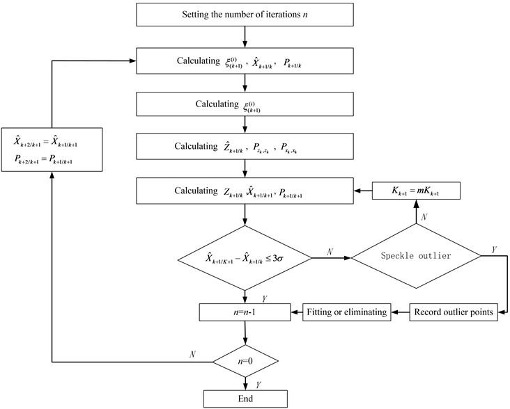
The flowchart of the adaptive Anti-Outlier UKF and GA-BPNN is shown in Fig. 2.
4. Numerical simulation and experimental verification
4.1. Numerical simulation
Carsim and Matlab/Simulink software are used to conduct co-simulation experiments to verify the estimation algorithm. Carsim is a professional vehicle dynamics simulation software developed by the Mechanical Simulation Corporation (MSC) for feature oriented parametric modeling. It is aimed at making algorithm research and development in the automotive field, testing and shortening the vehicle cycle. Scholars or engineers can obtain operational results that can highly simulate the response of actual vehicles through Carsim, and conduct more in-depth analysis on them.
Fig. 2Flowchart of adaptive Anti-Outlier UKF and GA-BPNN
The main interface of Carsim consists of three parts:
Database. The database includes databases of the entire vehicle model, driver model, and external environment (road surface information, environmental wind information, etc.). These databases comprehensively consider the human vehicle road factors of the automotive operating environment. During the operation, you can either default to an already existing database or create a new database.
Model solver. This section is the core part of Carsim operation solving, where users can set simulation termination conditions, simulation step size, and other information. It can also be easily connected to Matlab/Simulink, C language, and VB language.
Post-processing. Carsim software has powerful post-processing capabilities. During its operation, the user can choose to analyze quantitatively the curve of a specific characteristic changing over time or other parameters, or observe the response of the vehicle visually and vividly through simulation animations. In general, Carsim is easy to use, its graphical interface is easy to operate, and data visualization is powerful. The accuracy of its mathematical model has been recognized by academia and the industry, because the software has excellent scalability, which can be easily integrated into Matlab/Simulink, C language, VB and other simulation environments.
The key parameters of the vehicle are shown in Table 1.
Table 1Simulation parameters
Parameter | Value |
(kg) | 1522 |
(kg∙m2) | 2430 |
(m) | 1.47 |
(m) | 1.08 |
(m) | 1.53 |
(m) | 1.56 |
The computing platform comprises a MacBook Air (Intel Core i5-5250U 1.6 GHz, Windows 10 Enterprise Edition) with MATLABR2009a. The BPNN is set as: the structure has 2 nodes in the input layer; 5 nodes in the hidden layer, and 1 node in the output layer, with a total of 15 nodes. And the running interval is 1 s.
Fig. 3Longitudinal velocity simulation
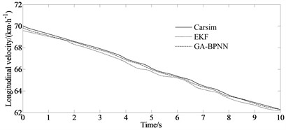
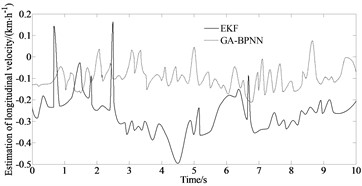
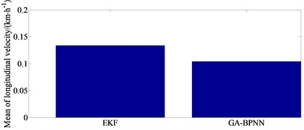
Fig. 3 compares and analyzes the estimated longitudinal velocity using the traditional EKF algorithm and the GA-BPNN algorithm proposed in this paper with the Carsim output parameter values. From Fig. 3, it can be observed that the estimation performance of the GA-BPNN algorithm is significantly better than that of EKF, with the maximum error of only 0.1 km/h. The numerical fluctuations can be stable and close to the actual values. The maximum error of EKF method reaches 0.113 km/h. Its estimated values are always near the actual values with very small errors, while the traditional EKF algorithm exhibits divergence at certain times.
Fig. 4Yaw rate simulation
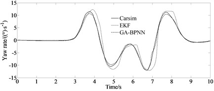
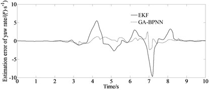
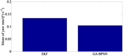
Fig. 4 compares and analyzes the estimated yaw rate using the traditional EKF algorithm and the GA-BPNN algorithm proposed in this paper with the Carsim output parameter values. From Fig. 4, it can be observed that the estimation performance of the GA-BPNN algorithm is significantly better than that of EKF. Traditional EKF exhibits more than one divergence phenomenon in 10 seconds, while the GA-BPNN algorithm maintains good convergence, with its estimated value located near the actual value, with the maximum error of only 0.1 (°/s), so the numerical fluctuation can be in a stable state.
Fig. 5Side slip angle simulation
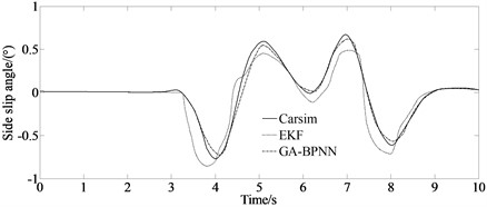
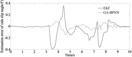
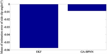
Fig. 5 compares and analyzes the estimated side slip angle using the traditional EKF algorithm and the GA-BPNN algorithm proposed in this paper with the Carsim output parameter values. From Fig. 5, it can be observed that the estimation performance of the GA-BPNN algorithm is significantly better than that of EKF. According to the simulation results, it can be concluded that the GA-BPNN method can correct the noise covariance through the involvement of parameter optimization estimation methods. Therefore, the GA-BPNN algorithm has excellent estimation accuracy and good convergence, which can effectively solve the problem of vehicle driving state estimation when the noise covariance is not accurately obtained.
The mean absolute error (MAE) and root mean square error (RMSE) are considered to verify the estimation accuracy of the proposed algorithm.
Table 2MAE and RMSE indicators of two algorithms
Evaluation index | State value | EKF | GA-BPNN |
MAE | (m/s) | 0.321 | 0.142 |
(m/s) | 0.192 | 0.0465 | |
(rad/s) | 0.323 | 0.0179 | |
RMSE | (m/s) | 0.354 | 0.139 |
(m/s) | 0.251 | 0.0518 | |
(rad/s) | 0.422 | 0.0219 |
From Table 2, it can be seen more intuitively that the estimation accuracy of the GA-BPNN algorithm is significantly higher than that of the EKF method.
4.2. Experimental verification
According to BS ISO 3888-2002, a double lane change test is carried out to verify the algorithm effectiveness. The main measurement devices are shown in Fig. 6. And the real test vehicle is shown in Fig. 7.
Fig. 6Measurement devices
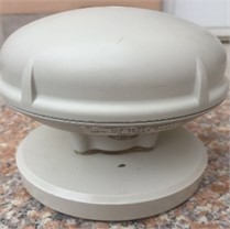
a) GPSSD-20 speed instrument
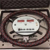
b) Steering torque/angle tester
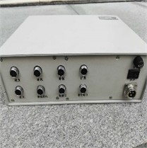
c) AM-2800 vehicle comprehensive performance test system
Fig. 7Real test vehicle
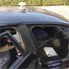
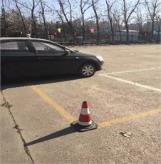
Fig. 8 depicts a comparison of the estimated and test values.
It can be seen from Fig. 8 that due to the existence of the vehicle dynamics model, tire model and sensor measurement errors, the errors of the longitudinal velocity, yaw rate and side slip angle appear as estimated. But the overall estimation effect is good, and it maintains a good consistency with the actual measured value indicating the good estimation accuracy and robustness of the proposed algorithm.
5. Conclusions
A 3-DOF vehicle model based on the longitudinal vehicle speed, yaw rate, and side slip angle is constructed, taking into account the nonlinear relationship between longitudinal vehicle speed and traditional vehicle state parameters to solve more rigorously the problem of vehicle state estimation. The UKF algorithm is improved by introducing a BP neural network improved by the genetic algorithm (GA-BPNN) to regulate and correct the global error and to improve the estimation accuracy of the UKF method. And the simulation has verified that this algorithm could provide more accurate vehicle state estimation in environments with inaccurate noise covariance. And also, compared with the traditional method, the simulation results indicate that the estimation performance of the GA-BPNN algorithm is significantly better than that of EKF. The proposed algorithm exhibits excellent characteristics such as clear physical meaning of states, good real-time performance. It plays an irreplaceable role in real-time and signal post-processing and has broad application prospects. In the future, the algorithm stability and the practical implementation of the proposed method require further in-depth research. And also, the weight optimization of the genetic algorithms has to be addressed with an intensive study.
Fig. 8Comparison of estimated and test values
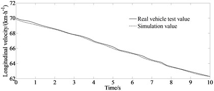
a) Test and estimated values of longitudinal velocity
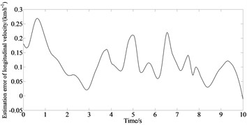
b) Estimation error of longitudinal velocity
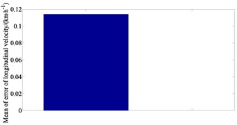
c) Mean value of estimation error of longitudinal velocity
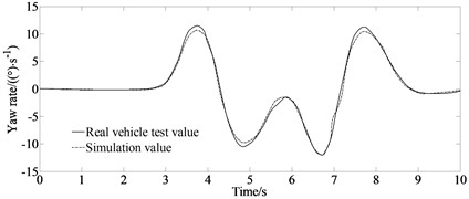
d) Test and estimated values of yaw rate
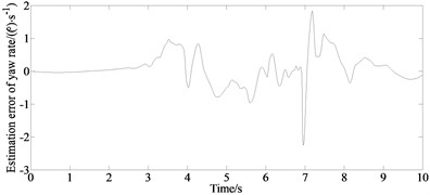
e) Estimation error of yaw rate
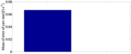
f) Mean value of estimation error of yaw rate
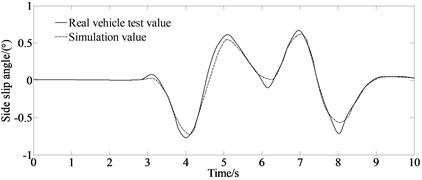
g) Test and estimated values of side slip angle
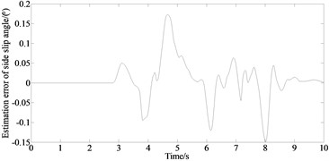
h) Estimation error of side slip angle
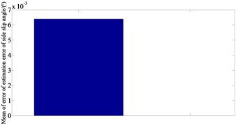
i) Mean value of estimation error of side slip angle
References
-
Y. Liu and D. Cui, “Vehicle state and parameter estimation based on double cubature Kalman filter algorithm,” Journal of Vibroengineering, Vol. 24, No. 5, pp. 936–951, Aug. 2022, https://doi.org/10.21595/jve.2022.22356
-
D. Tian, L. Jin, Z. Zhang, and H. Li, “Vehicle state estimation based on multidimensional information fusion,” IEEE Access, Vol. 10, pp. 76220–76232, 2022, https://doi.org/10.1109/access.2022.3192124
-
Z. Yu, X. Hou, B. Leng, and Y. Huang, “Mass estimation method for intelligent vehicles based on fusion of machine learning and vehicle dynamic model,” Autonomous Intelligent Systems, Vol. 2, No. 1, pp. 1–10, Dec. 2022, https://doi.org/10.1007/s43684-022-00020-8
-
S. Cai, H. Ding, Y. Hu, L. Zhang, Q. Li, and H. Chen, “Open-source dataset of vehicle state for an electric vehicle on a low-adhesion road,” Science China Information Sciences, Vol. 65, No. 3, pp. 1–2, Mar. 2022, https://doi.org/10.1007/s11432-020-3200-5
-
A. Habibnejad Korayem, A. Khajepour, and B. Fidan, “A review on vehicle-trailer state and parameter estimation,” IEEE Transactions on Intelligent Transportation Systems, Vol. 23, No. 7, pp. 5993–6010, Jul. 2022, https://doi.org/10.1109/tits.2021.3074457
-
Y. Xiang, Y. He, Y. Luo, D. Bu, W. Kong, and J. Chen, “Recognition model of sideslip of surrounding vehicles based on perception information of driverless vehicle,” IEEE Intelligent Systems, Vol. 37, No. 2, pp. 79–91, Mar. 2022, https://doi.org/10.1109/mis.2021.3110212
-
P. Xu, X. Hu, B. Liu, T. Ouyang, and N. Chen, “Hierarchical estimation model of state-of-charge and state-of-health for power batteries considering current rate,” IEEE Transactions on Industrial Informatics, Vol. 18, No. 9, pp. 6150–6159, Sep. 2022, https://doi.org/10.1109/tii.2021.3131725
-
Z. Xue, S. Cheng, L. Li, Z. Zhong, and H. Mu, “A robust unscented m-estimation-based filter for vehicle state estimation with unknown input,” IEEE Transactions on Vehicular Technology, Vol. 71, No. 6, pp. 6119–6130, Jun. 2022, https://doi.org/10.1109/tvt.2022.3163207
-
Y. Zhang, M. Li, Y. Zhang, Z. Hu, Q. Sun, and B. Lu, “An enhanced adaptive unscented Kalman filter for vehicle state estimation,” IEEE Transactions on Instrumentation and Measurement, Vol. 71, pp. 1–12, 2022, https://doi.org/10.1109/tim.2022.3180407
-
Z. Qin, L. Chen, M. Hu, and X. Chen, “A lateral and longitudinal dynamics control framework of autonomous vehicles based on multi-parameter joint estimation,” IEEE Transactions on Vehicular Technology, Vol. 71, No. 6, pp. 5837–5852, Jun. 2022, https://doi.org/10.1109/tvt.2022.3163507
-
J. Zubaca, M. Stolz, R. Seeber, M. Schratter, and D. Watzenig, “Innovative interaction approach in IMM filtering for vehicle motion models with unequal states dimension,” IEEE Transactions on Vehicular Technology, Vol. 71, No. 4, pp. 3579–3594, Apr. 2022, https://doi.org/10.1109/tvt.2022.3146626
-
A. N. Muhammed Hafiz and S. P. Anusha, “Real-time delay estimation model for mixed traffic conditions using RFID detections as data source,” Transportation in Developing Economies, Vol. 8, No. 2, pp. 1–10, Oct. 2022, https://doi.org/10.1007/s40890-022-00157-4
-
W. Zhang, L. Wang, L. Wang, C. Liao, and Y. Zhang, “Joint state-of-charge and state-of-available-power estimation based on the online parameter identification of lithium-ion battery model,” IEEE Transactions on Industrial Electronics, Vol. 69, No. 4, pp. 3677–3688, Apr. 2022, https://doi.org/10.1109/tie.2021.3073359
-
B. Jiang, H. Dai, and X. Wei, “A cell-to-pack state estimation extension method based on a multilayer difference model for series-connected battery packs,” IEEE Transactions on Transportation Electrification, Vol. 8, No. 2, pp. 2037–2049, Jun. 2022, https://doi.org/10.1109/tte.2021.3115597
-
W. Farag, “Self-driving vehicle localization using probabilistic maps and Unscented-Kalman filters,” International Journal of Intelligent Transportation Systems Research, Vol. 20, No. 3, pp. 623–638, Dec. 2022, https://doi.org/10.1007/s13177-022-00314-4
-
Y. Wang et al., “Tire road friction coefficient estimation: review and research perspectives,” Chinese Journal of Mechanical Engineering, Vol. 35, No. 1, pp. 1–11, Dec. 2022, https://doi.org/10.1186/s10033-021-00675-z
-
D. T. Le, D. T. Nguyen, N. D. Le, and T. L. Nguyen, “Traction control based on wheel slip tracking of a quarter-vehicle model with high-gain observers,” International Journal of Dynamics and Control, Vol. 10, No. 4, pp. 1130–1137, Aug. 2022, https://doi.org/10.1007/s40435-021-00881-6
-
K. Biswas and I. Kar, “Validating observer based on-line slip estimation for improved navigation by a mobile robot,” International Journal of Intelligent Robotics and Applications, Vol. 6, No. 3, pp. 564–575, Sep. 2022, https://doi.org/10.1007/s41315-021-00216-w
-
J. Wang, Y. Dong, S. Zhao, and Z. Zhang, “A high-precision vehicle detection and tracking method based on the attention mechanism,” Sensors, Vol. 23, No. 2, p. 724, Jan. 2023, https://doi.org/10.3390/s23020724
-
L. Gao, L. Xiong, X. Xia, Y. Lu, Z. Yu, and A. Khajepour, “Improved vehicle localization using on-board sensors and vehicle lateral velocity,” IEEE Sensors Journal, Vol. 22, No. 7, pp. 6818–6831, Apr. 2022, https://doi.org/10.1109/jsen.2022.3150073
-
H. Ding, H. Pan, H. Bai, X. Zheng, J. Chen, and W. Zhang, “Driving strategy of connected and autonomous vehicles based on multiple preceding vehicles state estimation in mixed vehicular traffic,” Physica A: Statistical Mechanics and its Applications, Vol. 596, p. 127154, Jun. 2022, https://doi.org/10.1016/j.physa.2022.127154
-
P. Bruni, S. Ceresara, Y. Li, Q. Lin, B. Musso, and A. Zichichi, “Design study of a phi 19.5*36 m superconducting solenoid (for supercollider Multi-TeV detector),” in IEEE Transactions on Magnetics, Vol. 27, No. 2, pp. 1969–1972, Mar. 1991, https://doi.org/10.1109/20.133590
About this article

This research was supported by the Science and Technology Program Foundation of Weifang under Grant 2015GX007. Moreover, this research was financially supported by the Open Research Fund from the State Key Laboratory of Rolling and Automation, Northeastern University, under Grant 2021RALKFKT008. The first author gratefully acknowledges these supports.
The datasets generated during and/or analyzed during the current study are available from the corresponding author on reasonable request.
Yingjie Liu: mathematical model and the simulation techniques. Dawei Cui: spelling and grammar checking as well as virtual validation. Wen Peng: experimental validation.
The authors declare that they have no conflict of interest.
