Time domain response analysis of multi-flow channel hydraulic mount

Lin, Zhihong; Wang, Chunrong; Chen, Yunxiao; Wu, Mingzhong; Zheng, Feijie; Wei, Jian

doi:10.21595/jve.2023.22940

Journal of Vibroengineering

Browse Journal

Submit article

Published: 05 December 2023

Check for updates

Time domain response analysis of multi-flow channel hydraulic mount

Zhihong Lin¹

Chunrong Wang²

Yunxiao Chen³

Mingzhong Wu⁴

Feijie Zheng⁵

Jian Wei⁶

^{1, 2, 5, 6}School of Mechanical and Electrical Engineering, Sanming University, Sanming Fujian, 365004, China

^{3, 4}College of Mechanical Engineering and Automation, HuaQiao University, Xiamen, 361021, China

Corresponding Author:

Zhihong Lin

Cite the article Download PDF

Downloads 58

Abstract

In order to analyze the effect of the combination of long and short inertia channels and orifice flow channels on the time domain response of hydraulic mounts. Firstly, six hydraulic mounts with different combinations of inertia channels and orifice flow channels are proposed. And then, the transfer functions of dynamic stiffness and upper chamber pressure for six structures of hydraulic mounts are derived using the lumped parameter method. Next, the time domain analytic formulas for the transfer force and upper chamber pressure for six structural hydraulic mounts under steady-state excitation and step excitation are obtained using the convolution method. Finally, the analytical formula is compared with the hydraulic mount’s model built by AMEsim; Meanwhile, the effects of inertia terms of inertia channels, damping, and damping of orifice flow channels on hydraulic mounts transfer forces are analyzed; Analyze the effect of transfer force variation and excitation amplitude on hydraulic mounts damping for different configurations of structures. Research shows that inertia channels and orifice flow channels directly affect the low-frequency dynamic characteristics of hydraulic mounts. At the same time, the effective damping height of the hydraulic mounts depends on the excitation amplitude.

Highlights

six hydraulic mounts with different combinations of inertia channels and orifice flow channels are proposed. And then, the transfer functions of dynamic stiffness and upper chamber pressure for six structures of hydraulic mounts are derived using the lumped parameter method.
the time domain analytic formulas for the transfer force and upper chamber pressure for six structural hydraulic mounts under steady-state excitation and step excitation are obtained using the convolution method.
the analytical formula is compared with the hydraulic mount's model built by AMEsim; Meanwhile, the effects of inertia terms of inertia channels, damping, and damping of orifice flow channels on hydraulic mounts transfer forces are analyzed.

1. Introduction

The mounts are vibration isolation elements connected between the engine and the vehicle frame, supporting the static engine load-bearing capacity, isolating the engine vibration transmitted to the vehicle frame, and reducing the impact of road impact on the engine, limiting the engine movement space. The ideal powertrain components should exhibit large stiffness and large damping at low frequencies and low stiffness and low damping at high frequencies to achieve vehicle vibration isolation performance under different operating conditions [1]. Due to the strong frequency and amplitude dependence of the mounts themselves, passive hydraulic mounts that are superior to passive rubber mounts are proposed [2]. Meanwhile, semi-active or active mounts have recently become a major research topic [3-5]. However, passive hydraulic mounts are still widely used due to their simple design and low cost.

Singh [6] proposed a linear time-invariant model with aggregate mechanics and fluid cells and validated the model by comparing dynamic stiffness predictions with experimental data for a frequency range of 1-50 Hz, emphasizing the modeling of free and fixed types of decouplers. Tiwari [7] conducted an experimental study on the hydraulic mount of an inertial channel and free-floating decoupler, identifying the inertial channel resistance, the top and bottom chamber compliance, and the effective piston area of the top chamber, and characterizing it in the frequency and time domains. Yoon and Singh [8, 9] proposed an indirect method based on the quasi-linear fluid system formulation to estimate the power transmitted by a fixed or free decoupled hydraulic mount on a rigid base to compensate for the inaccuracy of the mechanical system model. Farzad [10] proposed a variable stiffness decoupler membrane structure to replace the conventional decoupled membrane channel, and the new decoupled membrane structure can adjust the membrane stiffness according to the excitation frequency to achieve the optimal vibration isolation performance of the mounts. Liao [11] used ABAQUS software to build a fluid-structure coupling model of multi-inertial channel hydraulic mounts and to identify the structural parameters.

Studies on multi-inertia channel hydraulic mounts or bushings are mainly conducted by Zhang [12] to study the effects of the number, size, and length of inertia channels on the low-frequency dynamic performance of hydraulic mounts, revealing that different numbers of inertia channels can change the relationship between the stiffness and loss angle of hydraulic mounts and the excitation frequency. Yang [13, 14] established a multi-inertia channel-multi-throttle orifice type hydraulic bushing set parameter model, and derived formulas for stiffness and loss angle to analyze the relationship between the dynamic characteristics of multi-channel hydraulic bushings and the number of channels. It was shown that increasing the number of inertia channels and/or orifices can significantly improve the dynamic stiffness, the amplitude of loss angle, and the corresponding frequency of the bushing, thus greatly improving the performance of the bushing. Tan Chai [15-17] developed a controllable conceptual hydraulic bushing model with two parallel unequal inertia channels and a flow control unit to analyze the dynamic and time-domain characteristics of a multi-flow channel bushing numerically and experimentally. Lu [18] studied the $n =$ 2 inertial channels mainly to derive a linear set of total parameters model for the hydraulic mount with $n =$ 2 and analyzed its dynamic characteristics. Li [19] proposed an inertial channel optimization method based on a linearized low-frequency model excluding the effect of decoupling membranes, considering multiple arrangements of inertial channel and orifice combinations. Also, the predictions of the hydraulic mounts model were referred to the relevant references by Shishegaran [20-30]. It is shown that the use of two configurations can reduce the relative engine and body displacement transmissibility. Although studies on the time and frequency domain characteristics of multi-inertia channel hydraulic bushings have been reported, there are still some differences between the hydraulic bushing and hydraulic mount characteristics [31], and the time-domain characteristics of multi-flow channel hydraulic mounts cannot be well understood by hydraulic bushing time-domain analysis. Meanwhile, although the analysis of dynamic characteristics of multi-flow channel hydraulic mounts has been studied, the frequency domain characteristics and transient characteristics of multi-flow channel hydraulic mounts considering various combinations simultaneously have not been reported yet.

Based on the above review, the specific research objectives of this paper are as follows: To propose a lumped parameter model of the hydraulic mounts for 6 configurations of long and short inertia channels combined with orifice flow channels, and to solve the corresponding dynamic stiffness and upper chamber pressure transfer functions. Solve the time domain expressions for the steady-state response and ideal step response of the transfer force and upper chamber pressure based on the derived dynamic stiffness and upper chamber pressure transfer functions. The effects of upper chamber compliance, fluid viscosity, inertia, and damping of long and short inertia channels and orifice flow channel damping on hydraulic mount transfer force are analyzed based on time-domain expressions, and the effect of excitation amplitude on damping is also analyzed.

2. Hydraulic mount prototype study

2.1. Hydraulic mount structure

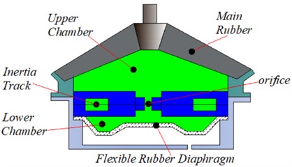
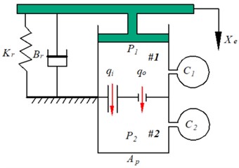
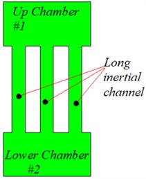
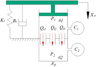
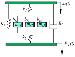
Fig. 1 shows a schematic diagram of the hydraulic mount, where Fig. 1(a) shows the structure of the passive hydraulic mount, and Fig. 1(b) shows the lumped parameter model of the passive hydraulic mount. In this case, the hydraulic mount structure includes an inertial channel and an orifice flow channel. The flow rates in the inertial and orifice flow channels are denoted by $q_{i}$ and $q_{o}$ , respectively. The rubber unit is modeled using the rubber stiffness $K_{r}$ and the viscous damping coefficient $B_{r}$ . The compliances of the upper and lower chambers of the hydraulic mount are $C_{1}$ and $C_{2}$ respectively, and the pressure of the upper chamber #1 is $P_{1}$ , and the pressure of the lower chamber #2 is $P_{2}$ . where the inertial channel and the orifice flow channel are represented by the fluid inertia $I_{i}$ and $I_{o}$ and the fluid resistance $R_{i}$ and $R_{o}$ , respectively.

Fig. 1Hydraulic mount: a) structure diagram, b) lumped parameter model

a)

b)

2.2. Hydraulic mount flow channel design with multiple configurations

From the literature [12, 32], it is known that increasing the number of hydraulic mount inertia channels can improve the peak frequency of the dynamic stiffness and loss angle of the mount, and the combination of different flow channels can broaden the range of hydraulic mount vibration isolation frequency. However, these literature studies are all from the mount frequency characteristics and rarely involve the analysis of multi-flow channel hydraulic mount time domain characteristics. To investigate common multi-flow hydraulic mounts, six prototype configurations as shown in Table 1 and Fig. 2 were analyzed.

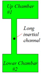
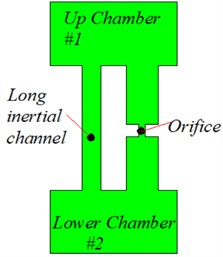
Fig. 2Multiple configurations of the hydraulic mount prototype a) single long inertia channel, configuration Z1, (L1= 212 mm, D1= 8.53 mm), configuration Z2 (L2=4L1, D2=D1); b) parallel combination of long inertia channel and orifice flow channel, configuration Z3 (L3=4L1, D3=D1, Lo1= 2 mm, Do1= 0.2 mm); configuration Z4 (L4=4L1, D4=D1, Lo2=Lo1, Do2=5Do1); c) parallel combination of three long inertia channels, configuration Z5 (L51=L52=L1, L53=4L1, D51=D52=D53=D1), configuration Z6 (L51=L52=L53=L1, D51=D52=D53=D1)

Multiple configurations of the hydraulic mount prototype a) single long inertia channel, configuration Z1, (L1= 212 mm, D1= 8.53 mm), configuration Z2 (L2=4L1, D2=D1); b) parallel combination of long inertia channel and orifice flow channel, configuration Z3 (L3=4L1, D3=D1, Lo1= 2 mm, Do1= 0.2 mm); configuration Z4 (L4=4L1, D4=D1, Lo2=Lo1, Do2=5Do1); c) parallel combination of three long inertia channels, configuration Z5 (L51=L52=L1, L53=4L1, D51=D52=D53=D1), configuration Z6 (L51=L52=L53=L1, D51=D52=D53=D1)

a)

b)

c)

The first configuration (named $Z_{1}$ , $Z_{2}$ ) hydraulic mount upper and lower chambers are connected only by long inertia channels, this structure is the most common at present. Where, the length of $Z_{1}$ inertia channel $L_{1} =$ 212 mm, the length of $Z_{2}$ inertia channel $L_{2} = 4 L_{1}$ , the diameter of $Z_{1}$ and $Z_{2}$ inertia channels are equal $D_{1} = D_{2} =$ 8.53 mm. In the second configuration (named $Z_{3}$ and $Z_{4}$ ), the upper and lower chambers of the hydraulic mount are connected in parallel by long inertia channels and orifice flow channel. Where $Z_{3}$ and $Z_{4}$ inertia channels have equal lengths and diameters, $L_{3} = L_{4} = 4 L_{1}$ , $D_{3} = D_{4} =$ 8.53 mm, respectively; The length of the $Z_{3}$ configuration orifice flow channel and $Z_{4}$ are equal to $L_{o 1} = L_{o 2} =$ 2 mm, the diameter of the $Z_{3}$ orifice flow channel is $D_{o 1} =$ 0.2 mm, and the diameter of the $Z_{4}$ orifice flow channel is $D_{o 2} =$ 1 mm. The third configuration (named $Z_{5}$ , $Z_{6}$ ) is a parallel combination of the number of long inertia channels $n =$ 3. Where the diameters of the $Z_{5}$ and $Z_{6}$ inertial channels are equal $D_{5} = D_{6} =$ 8.53 mm, $L_{51} = L_{52} = L_{1}$ , $L_{53} = 4 L_{1}$ in the $Z_{5}$ configuration; the lengths of the three inertial channels in the $Z_{6}$ configuration are equal $L_{61} = L_{62} = L_{63} = L_{1}$ .

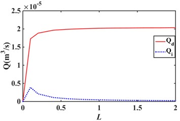
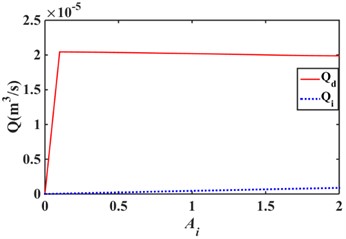
Fig. 3 shows the effect of variation in inertial channel length and cross-sectional area on the flow rate of the decoupler membrane channel. The decoupler membrane channel flow increases slightly with increasing inertial channel length. The flow rate of the decoupler membrane channel decreases slightly as the cross-sectional area of the inertial channel increases.

Table 1Study configuration: prototype hydraulic engine mounts with inertia channel and orifice flow channel

Design	$n$	Description (also see Fig. 2)
$Z_{1}$	1	Baseline configuration (A long inertia channel, $L_{1}$ , $D_{1}$ )
$Z_{2}$	1	A long inertia channel ( $L_{2} = 4 L_{1}$ , $D_{2} = D_{1}$ )
$Z_{3}$	2	Parallel combination of long inertia channel and orifice flow channel ( $L_{3} = 4 L_{1}$ , $D_{3} = D_{1}, L_{o 1}, D_{o 1}$ )
$Z_{4}$	2	Parallel combination of long inertia channel and orifice flow channel ( $L_{3} = 4 L_{1}$ , $D_{3} = D_{1}$ , $L_{o 2} = L_{o 1}$ , $D_{o 2} = 5 D_{o 1}$ )
$Z_{5}$	3	Long inertia channel parallel combination ( $L_{51} = L_{52} = L_{1}$ , $L_{53} = 4 L_{1}$ , $D_{51} = D_{52} = D_{53} = D_{1}$ )
$Z_{6}$	3	Long inertia channel parallel combination ( $L_{61} = L_{62} = L_{63} = L_{1}$ , $D_{51} = D_{52} = D_{53} = D_{1}$ )

Fig. 3Effect of hydraulic mount inertia channel length and cross-sectional area variation on decoupling membrane channel flow: a) length variation; b) cross-sectional area variation

Effect of hydraulic mount inertia channel length and cross-sectional area variation on decoupling membrane channel flow: a) length variation; b) cross-sectional area variation

a)

b)

2.3. AMEsim-based hydraulic mount study

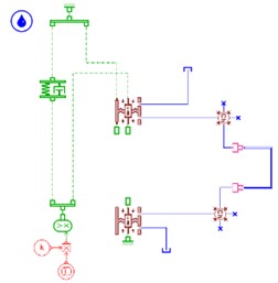
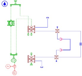
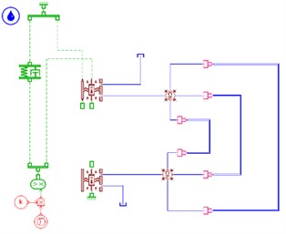
Fig. 4 shows the hydraulic mounts models of six configurations built using AMEsim software.

Fig. 4(a) shows the hydraulic mounts of $Z_{1}$ and $Z_{2}$ configurations, Fig. 4(b) shows the hydraulic mounts of $Z_{3}$ and $Z_{4}$ configurations, and Fig. 4(c) shows the hydraulic mounts of $Z_{5}$ and $Z_{6}$ configurations.

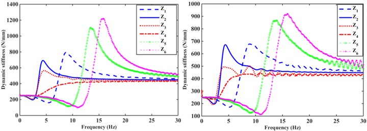
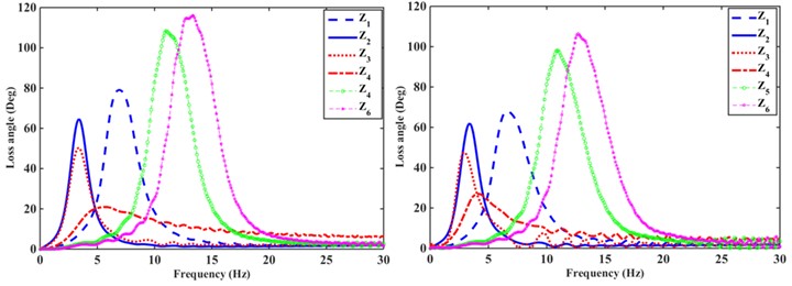
Build 6 hydraulic mounts configurations using AMEsim, and the dynamic characteristics of the combined inertial channel and orifice flow channel hydraulic mounts were simulated for the above six configurations. The test uses a sinusoidal displacement excitation $x_{e} (t) = A s i n ω t$ , where $A$ is the amplitude of the harmonic input and $f = ω / 2 π$ is the frequency of the excitation, where the unit is Hz. The transfer forces of the hydraulic mounts and the dynamic pressures $P_{1} (t)$ and $P_{2} (t)$ within the upper and lower chambers are calculated in 1 Hz increases between 1 and 30 Hz in $X_{e} =$ 0.3 mm, $X_{e} =$ 0.9 mm and, where $X_{e} = 2 A$ is the peak-to-peak (P-P) value. The calculated dynamic stiffness and loss angle for a given excitation amplitude $X_{e} =$ 0.3 mm and $X_{e} =$ 0.9 mm hydraulic mounts can be obtained as shown in Fig. 4. It is worth noting that configurations $Z_{5}$ and $Z_{6}$ exhibit greater dynamic stiffness and loss angle peak frequency. While configurations $Z_{3}$ and $Z_{4}$ show the smallest peak frequencies for dynamic stiffness and hysteresis angle, this is due to the inclusion of orifice flow channels in both configurations. Finally, the dynamic stiffness and loss angle of $Z_{1}$ and $Z_{2}$ are relatively small relative to the peak, due to the number of flow channels of one in the configuration. When the excitation amplitude $X_{e}$ is increased from 0.3 mm to 0.9 mm, the dynamic stiffness and hysteresis angle of the hydraulic mounts decrease, which is more obvious for $Z_{1}$ , $Z_{2}$ , $Z_{5}$ and $Z_{6}$ .

Fig. 4AMEsim hydraulic mount model: a) single inertia channel; b) combination of inertia channel and orifice flow channel; c) combination of 3 inertia channels

AMEsim hydraulic mount model: a) single inertia channel; b) combination of inertia channel and orifice flow channel; c) combination of 3 inertia channels

a)

b)

c)

Fig. 5Dynamic stiffness and loss angle of six configurations of hydraulic mount: a) Xe= 0.3 mm; b) Xe= 0.9 mm

a)

b)

3. Multi-flow channel hydraulic mount analysis model

3.1. Model I single inertia channel hydraulic mount

When the hydraulic mount is excited by $x_{e} (t)$ , applying the continuity equation to the fluid control hydraulic unit in combination with Fig. 1 and Fig. 1(a), the following Eq. (1)-(5) are obtained. Where the fluid inertia $I_{i}$ and the fluid resistance $R_{i}$ are expressed:

1

P_{1} (t) - P_{2} (t) = I_{i} q_{i} (t) + R_{i} q_{i} (t),

2

C_{1} {\dot{P}}_{1} (t) = A_{p} {\dot{x}}_{e} (t) - q_{i} (t),

3

C_{2} {\dot{P}}_{2} (t) = q_{i} (t),

4

I_{i} = \frac{ρ L}{A_{i}},

5

R_{i} = \frac{128 v i s L}{π D_{h}^{4}},

where $ρ$ is the density of the fluid, $L$ is the length of the flow channel, $A_{i}$ is the cross-sectional area of the flow channel, and $v$ is the viscosity of the fluid, $D_{h}$ is the equivalent “hydraulic diameter” of the flow channel. The first term on the right side of Eq. (1) is the pressure drop due to the fluid in the inertial channel due to inertia; the second term on the right side is the pressure drop due to the viscous damping of the fluid in the inertial channel.

Therefore, the hydraulic mount transfer force $F_{T}$ under external excitation $X_{e}$ is defined as follows:

6

F_{T} = B_{r} {\dot{x}}_{e} (t) + K_{r} x_{e} (t) + A_{p} P_{1} (t) .

Then, by Laplace transformation of Eq. (6), the expressions for the variation of the transfer complex stiffness and the upper chamber pressure with the excitation amplitude for a single-flow channel hydraulic mount are obtained as follows:

7

K_{d y n} (s) = \frac{F_{T}}{x_{e}} (s) = K_{r} + B_{r} s + A_{p}^{2} K_{1} \frac{I_{i} s^{2} + R_{i} s + K_{2}}{I_{i} s^{2} + R_{i} s + K_{2} + K_{1}},

8

\frac{P_{1}}{x_{e}} (s) = A_{p} K_{1} \frac{I_{i} s^{2} + R_{i} s + K_{2}}{I_{i} s^{2} + R_{i} s + K_{2} + K_{1}} .

Since $1 / C_{1} = K_{1}$ , $1 / C_{2} = K_{2}$ , and $K_{1} ≫ K_{2}$ . So, Eqs. (7) and (8) can be further simplified as follows:

9

K_{d y n} (s) = \frac{F_{T}}{x_{e}} (s) = K_{r} + B_{r} s + A_{p}^{2} K_{1} \frac{I_{i} s^{2} + R_{i} s}{I_{i} s^{2} + R_{i} s + K_{1}},

10

\frac{P_{1}}{x_{e}} (s) = A_{p} K_{1} \frac{I_{i} s^{2} + R_{i} s}{I_{i} s^{2} + R_{i} s + K_{1}} .

Eq. (9) and Eq. (10) can be simplified to a standard second-order system:

11

K_{d 1} (s) = \frac{F_{T}}{x_{e}} (s) = K_{r} + B_{r} s + λ \frac{s^{2} + 2 ς_{2} ω_{n 2} s}{s^{2} + 2 ς_{2} ω_{n 2} s + ω_{n 2}^{2}},

12

\frac{P_{1}}{x_{e}} (s) = A_{p} K_{1} \frac{I_{i} s^{2} + R_{i} s}{I_{i} s^{2} + R_{i} s + K_{1}} = A_{p} K_{1} \frac{s^{2} + 2 ς_{2} ω_{n 2} s}{s^{2} + 2 ς_{2} ω_{n 2} s + ω_{n 2}^{2}} .

Thus, Eq. (11) can be transformed into the following standard form, where $λ = A_{p}^{2} K_{1}$ , $τ = R_{i} / I_{i}$ :

13

K_{d 1} (s) = K_{r} + B_{r} s + λ \frac{(s + τ) s}{s^{2} + 2 ς_{2} ω_{n 2} s + ω_{n 2}^{2}},

14

G (s) = \frac{P_{1}}{x_{e}} (s) = A_{p} K_{1} \frac{(s + τ) s}{s^{2} + 2 ς_{2} ω_{n 2} s + ω_{n 2}^{2}},

where $ς_{2} = \sqrt{R_{i}^{2} / 4 K_{1} I_{i}}$ , $ω_{n 2} = \sqrt{K_{1} / I_{i}}$ .

3.2. Model II combined inertial channel and orifice flow channel hydraulic mount

According to Fig. 1 and Fig. 2(b), the fluid equation of the hydraulic mount subjected to displacement excitation $x_{e} (t)$ for the parallel combination of inertial channel and orifice flow channel can be obtained as shown below:

15

P_{1} - P_{2} = I_{i} {\dot{q}}_{i} + R_{i} q_{i},

16

P_{1} - P_{2} = R_{0} q_{0},

17

C_{1} {\dot{P}}_{1} = A_{p} {\dot{x}}_{e} - q_{i} - q_{0},

18

C_{2} {\dot{P}}_{2} = q_{i} + q_{0} .

In the equation, $R_{0}$ is the fluid resistance of the orifice flow channel. Since the inertia in the orifice flow channel is negligible, Eq. (16) only considers the viscous damping term resulting in the hydraulic mounts differential pressure change. Reference [33] shows that when the fluid is assumed to be in the form of laminar flow in the orifice flow channel, the fluid resistance of the orifice flow channel is solved for by the following expression:

19

R_{0} = \frac{50.4 v i s}{π D_{o}^{3}},

where, $D_{o}$ is the diameter of the orifice flow channel.

Thus, the hydraulic mounts parallel to the inertial channel and the orifice flow channel transfer the complex stiffness $K_{d 2} (s)$ and the variation of the upper chamber pressure with the excitation amplitude $G (s)$ defined as follows:

20

K_{d 2} (s) = \frac{F_{T}}{x_{e}} (s) = K_{r} + B_{r} s + A_{p}^{2} K_{1} \frac{I_{i} R_{0} s^{2} + (K_{2} I_{i} + R_{i} R_{0}) s + K_{2} (R_{i} - R_{0})}{I_{i} R_{0} s^{2} + (K_{2} I_{i} + R_{i} R_{0} + K_{1} I_{i}) s + (K_{2} + K_{1}) (R_{i} + R_{0})},

21

G (s) = \frac{P_{1}}{x_{e}} (s) = A_{p} K_{1} \frac{I_{i} R_{0} s^{2} + (K_{2} I_{i} + R_{i} R_{0}) s + K_{2} (R_{i} - R_{0})}{I_{i} R_{0} s^{2} + (K_{2} I_{i} + R_{i} R_{0} + K_{1} I_{i}) s + (K_{2} + K_{1}) (R_{i} + R_{0})} .

Since $1 / C_{1} = K_{1}$ , $1 / C_{2} = K_{2}$ , and $K_{1} ≫ K_{2}$ can be simplified by Eqs. (20) and (21) as follows:

22

K_{d y n} (s) = \frac{F_{T}}{x_{e}} (s) = K_{r} + B_{r} s + A_{p}^{2} K_{1} \frac{I_{i} R_{0} s^{2} + R_{i} R_{0} s}{I_{i} R_{0} s^{2} + (R_{i} R_{0} + K_{1} I_{i}) s + K_{1} (R_{i} + R_{0})},

23

G (s) = \frac{P_{1}}{x_{e}} (s) = A_{p} K_{1} \frac{I_{i} R_{0} s^{2} + R_{i} R_{0} s}{I_{i} R_{0} s^{2} + (R_{i} R_{0} + K_{1} I_{i}) s + K_{1} (R_{i} + R_{0})} .

So, reduced to the standard second-order system form shown:

24

K_{d y n - 2} (s) = \frac{F_{T}}{x_{e}} (s) = K_{r} + B_{r} s + λ \frac{s (s + κ)}{s^{2} + 2 ς_{2} ω_{n 2} s + ω_{n 2}^{2}},

25

G (s) = \frac{P_{1}}{x_{e}} (s) = A_{p} K_{1} (\frac{s (s + κ)}{s^{2} + 2 ς_{2} ω_{n 2} s + ω_{n 2}^{2}}),

where the expressions for $ω_{n 2}$ , $ς_{2}$ , $κ$ and $F$ are shown:

ω_{n 2} = \sqrt{\frac{(R_{i} + R_{0}) K_{1}}{I_{i} R_{0}}}, ς_{2} = \frac{(R_{i} R_{0} + K_{1} I_{i})}{2} \sqrt{\frac{1}{K_{1} I_{i} R_{0} (R_{i} + R_{0})}}, κ = \frac{R_{i}}{I_{i}}, λ = A_{p}^{2} K_{1} .

3.3. Model III parallel combination of 3 flow channel hydraulic mount

To easily solve for the multi-inertia channel hydraulic mount transfer complex stiffness $K_{d 3} (s)$ and the upper chamber pressure variation $G (s)$ with excitation amplitude for the $Z_{5}$ and $Z_{6}$ configurations. The lumped parameter model of the multi-inertia channel hydraulic mounts with $Z_{5}$ and $Z_{6}$ configurations of Fig. 6(a) is equated to the equivalent mechanical model of Fig. 6(b). Because the cross-sectional area of the hydraulic mount inertia channel is much smaller than the equivalent cross-sectional area of the rubber main spring, when the fluid flows through the inertia channel, the fluid velocity is amplified to play the role of vibration attenuation, the literature [6] referred to it as a velocity amplification of large absorbing array.

Fig. 6Multi-inertia channel hydraulic mount: a) lumped parameter model, b) equivalent mechanical model

a)

b)

According to Fig. 6(a), the mathematical model equation of the lumped parameters of the multi-inertia channel hydraulic mounts can be obtained as follows:

26

C_{1} {\dot{P}}_{1} = A_{p} {\dot{x}}_{e} - q_{i 1} - q_{i 2} - q_{i 3},

27

C_{2} {\dot{P}}_{2} = q_{i 1} + q_{i 2} + q_{i 3},

28

P_{1} - P_{2} = I_{i 1} {\ddot{q}}_{i 1} + R_{i 1} {\dot{q}}_{i 1},

29

P_{1} - P_{2} = I_{i 2} {\ddot{q}}_{i 2} + R_{i 2} {\dot{q}}_{i 2},

30

P_{1} - P_{2} = I_{i 3} {\ddot{q}}_{i 3} + R_{i 3} {\dot{q}}_{i 3},

31

F_{T} = K_{r} x_{e} + B_{e} x_{e} + A_{p} P_{1},

32

F_{T} = K_{r} x_{e} + B_{e} x_{e} + A_{p} P_{1},

where, $q_{i 1}$ , $q_{i 2}$ , $q_{i 3}$ are the flow rate through the three inertia channels of configuration $Z_{5}$ and $Z_{6}$ respectively, $I_{i 1}$ , $I_{i 2}$ , $I_{i 3}$ are the inertia flow through the three inertia channels respectively, $R_{i 1}$ , $R_{i 2}$ , $R_{i 3}$ are the liquid resistance flow through the three inertia channels respectively.

In Fig. 6(b), $k_{1} = A_{p}^{2} / C_{1}$ is the equivalent linear stiffness of the upper chamber of the hydraulic mount, $k_{2} = A_{p}^{2} / C_{2}$ is the equivalent linear stiffness of the lower chamber of the hydraulic mount, $b_{i n}$ ( $n =$ 1, 2, 3) is the equivalent damping of the fluid in the inertia channel of the hydraulic mount, and $m_{i n}$ ( $n =$ 1, 2, 3) is the equivalent mass of the fluid in the inertia channel of the hydraulic mount [34]. It is known that the flow rate $q = A_{i} {\dot{x}}_{i}$ , where $A_{i}$ is the cross-sectional area of the inertial channel and ${\dot{x}}_{i}$ is the average flow velocity of the fluid in the inertial channel. Therefore, Eqs. (32-35) can be written as shown in the following equation:

33

\frac{1}{C_{1}} (A_{p} x_{e} - A_{i 1} x_{i 1} - A_{i 2} x_{i 2} - A_{i 3} x_{i 3}) - \frac{1}{C_{2}} (A_{i 1} x_{i 1} + A_{i 2} x_{i 2} + A_{i 3} x_{i 3}) = I_{i 1} A_{i 1} {\ddot{x}}_{i 1} + R_{i 1} A_{i 1} {\dot{x}}_{i 1},

34

\frac{1}{C_{1}} (A_{p} x_{e} - A_{i 1} x_{i 1} - A_{i 2} x_{i 2} - A_{i 3} x_{i 3}) - \frac{1}{C_{2}} (A_{i 1} x_{i 1} + A_{i 2} x_{i 2} + A_{i 3} x_{i 3}) = I_{i 2} A_{i 2} {\ddot{x}}_{i 2} + R_{i 2} A_{i 2} {\dot{x}}_{i 2},

35

\frac{1}{C_{1}} (A_{p} x_{e} - A_{i 1} x_{i 1} - A_{i 2} x_{i 2} - A_{i 3} x_{i 3}) - \frac{1}{C_{2}} (A_{i 1} x_{i 1} + A_{i 2} x_{i 2} + A_{i 3} x_{i 3}) = I_{i 3} A_{i 3} {\ddot{x}}_{i 3} + R_{i 3} A_{i 3} {\dot{x}}_{i 3},

36

F_{T} = K_{r} x_{e} + B_{e} x_{e} + A_{p} P_{1} = K_{r} x_{e} + B_{e} x_{e} + \frac{1}{C_{1}} A_{p} (A_{p} x_{e} - A_{i 1} x_{i 1} - A_{i 2} x_{i 2} - A_{i 3} x_{i 3}),

where, $A_{i 1}$ , $A_{i 2}$ , $A_{i 3}$ are the cross-sectional areas of the three inertial channels in configurations $Z_{5}$ and $Z_{6}$ , and $x_{i 1}$ , $x_{i 2}$ , $x_{i 3}$ are the displacements of the fluid flowing through the three inertial channels in configurations $Z_{5}$ and $Z_{6}$ , respectively.

Combining the equivalent mechanical model of the multi-inertia channel hydraulic mount in Fig. 6(b) and the literature [2] the Eqs. (33-36) can be written as follows:

37

k_{1} (x_{e} - x_{i 1} - x_{i 2} - x_{i 3}) - k_{2} (x_{i 1} + x_{i 2} + x_{i 3}) = I_{i 1} A_{p}^{2} {\ddot{x}}_{i 1} + R_{i 1} A_{p}^{2} {\dot{x}}_{i 1},

38

k_{1} (x_{e} - x_{i 1} - x_{i 2} - x_{i 3}) - k_{2} (x_{i 1} + x_{i 2} + x_{i 3}) = I_{i 2} A_{p}^{2} {\ddot{x}}_{i 2} + R_{i 2} A_{p}^{2} {\dot{x}}_{i 2},

39

k_{1} (x_{e} - x_{i 1} - x_{i 2} - x_{i 3}) - k_{2} (x_{i 1} + x_{i 2} + x_{i 3}) = I_{i 3} A_{p}^{2} {\ddot{x}}_{i 3} + R_{i 3} A_{p}^{2} {\dot{x}}_{i 3},

40

F_{T} = K_{r} x_{e} + B_{e} x_{e} + k_{1} (x_{e} - x_{i 1} - x_{i 2} - x_{i 3}) .

Because $C_{1} ≪ C_{2}$ , The equivalent masses of the three inertia channels of the hydraulic mounts of the $Z_{5}$ and $Z_{6}$ structures are $m_{i 1} = I_{i 1} A_{p}^{2}$ , $m_{i 2} = I_{i 2} A_{p}^{2}$ , $m_{i 3} = I_{i 3} A_{p}^{2}$ , and the equivalent damping of the three inertial channels of the hydraulic mounts of the $Z_{5}$ and $Z_{6}$ are $b_{i 1} = R_{i 1} A_{p}^{2}$ , $b_{i 2} = R_{i 2} A_{p}^{2}$ , $b_{i 3} = R_{i 3} A_{p}^{2}$ respectively. Therefore, Eqs. (37)-(39) can be further simplified as shown below:

41

K_{1} (x_{e} - x_{i 1} - x_{i 2} - x_{i 3}) = m_{i 1} {\ddot{x}}_{i 1} + b_{i 1} {\dot{x}}_{i 1},

42

K_{1} (x_{e} - x_{i 1} - x_{i 2} - x_{i 3}) = m_{i 2} {\ddot{x}}_{i 2} + b_{i 2} {\dot{x}}_{i 2},

43

K_{1} (x_{e} - x_{i 1} - x_{i 2} - x_{i 3}) = m_{i 3} {\ddot{x}}_{i 3} + b_{i 3} {\dot{x}}_{i 3} .

Referring to the literature [32], the equivalent mass and equivalent damping of the inertial channel can be expressed as follows:

44

R_{e q} = \frac{Π_{i = 1}^{3} R_{i i}}{\sum_{i = 1}^{3} (R_{i i})} = \frac{R_{i 1} R_{i 2} R_{i 3}}{R_{i 1} + R_{i 2} + R_{i 3}} \Leftrightarrow b_{e q} = A_{p}^{2} R_{e q},

45

I_{e q} = \frac{Π_{i = 1}^{3} R_{i i}}{\sum_{i = 1}^{3} (R_{i i})} = \frac{R_{i 1} R_{i 2} R_{i 3}}{R_{i 1} + R_{i 2} + R_{i 3}} \Leftrightarrow m_{e q} = A_{p}^{2} I_{e q} .

Therefore, the Eqs. (40-43) can be reduced to the following expression:

46

K_{1} (x_{e} - x_{e q}) = m_{e q} {\ddot{x}}_{e q} + b_{e q} {\dot{x}}_{e q},

47

F_{T} = K_{r} x_{e} + B_{e} x_{e} + A_{p} P_{1} = K_{r} x_{e} + B_{e} x_{e} + k_{1} (x_{e} - x_{e q}) .

As a result, the transfer function expressions for the transfer complex stiffness and the upper chamber pressure variation with excitation for the multi-inertia channel hydraulic mounts of $Z_{5}$ and $Z_{6}$ structures are as follows:

48

\frac{F_{T}}{x_{e}} (s) = K_{r} + B_{r} s + \frac{k_{1} m_{e q} s^{2} + k_{1} b_{e q} s}{m_{e q} s^{2} + b_{e q} s + k_{1}},

49

G (s) = \frac{P_{1}}{x_{e}} (s) = \frac{k_{1}}{A_{p}} \frac{m_{e q} s^{2} + b_{e q} s}{m_{e q} s^{2} + b_{e q} s + k_{1}} .

Therefore, the expressions for Eqs. (48) and (49) reduced to a standard second-order system are shown below:

50

K_{d 3} (s) = \frac{F_{T}}{x_{e}} (s) = K_{r} + B_{r} s + λ \frac{s (s + κ)}{s^{2} + 2 ς_{2} ω_{n 2} s + ω_{n 2}^{2}},

51

G (s) = \frac{P_{1}}{x_{e}} (s) = \frac{k_{1}}{A_{p}} \frac{s (s + κ)}{s^{2} + 2 ς_{2} ω_{n 2} s + ω_{n 2}^{2}},

where the expressions for $κ$ , $ω_{n 2}$ and $ς_{2}$ are as follows:

κ = \frac{b_{e q}}{m_{e q}}, ω_{n 2} = \sqrt{\frac{K_{1}}{m_{e q}}}, ς_{2} = \frac{b_{e q}}{2} \sqrt{\frac{1}{K_{1} m_{e q}}}, λ = k_{1} .

The key parameters of the hydraulic mount can be obtained by combining model I, model II and mode III as shown in Table 2.

Table 2Key parameters of the system for the analytical model.

System parameters	Model I	Model II	Mode III
$λ$	$A_{p}^{2} K_{1}$	$A_{p}^{2} K_{1}$	$k_{1}$
$κ$	$\frac{R_{i}}{I_{i}}$	$\frac{R_{i}}{I_{i}}$	$\frac{b_{e q}}{m_{e q}}$
$ω_{n 2}$	$\sqrt{\frac{K_{1}}{I_{i}}}$	$\sqrt{\frac{(R_{i} + R_{0}) K_{1}}{I_{i} R_{0}}}$	$\sqrt{\frac{K_{1}}{m_{e q}}}$
$ς_{2}$	$\sqrt{\frac{R_{i}^{2}}{4 K_{1} I_{i}}}$	$\frac{(R_{i} R_{0} + K_{1} I_{i})}{2} \sqrt{\frac{1}{K_{1} I_{i} R_{0} (R_{i} + R_{0})}}$	$\frac{b_{e q}}{2} \sqrt{\frac{1}{K_{1} m_{e q}}}$

4. Multi-fluid hydraulic mount time domain analytical formula

4.1. Time domain steady-state harmonic response

To analyze the hydraulic mounts in Models I, II, and III configurations for steady-state harmonic response, the hydraulic mounts transfer the force $F_{T} (t)$ and the pressure $P_{1} (t)$ in the upper chamber, the specific derivation process was referred to the reference [15, 16]. According to the convolution of the bishop function:

52

L [x (t) * y (t)] = X (s) Y (s),

where $x (t) * y (t)$ is the mathematical expression of the convolution.

Therefore, the analytical equations of the transfer force $F_{T} (t)$ and the pressure $P_{1} (t)$ in the upper chamber under the steady-state harmonic response in the time domain for models I, II and III of the hydraulic mount configurations can be solved according to Eq. (52), which is expressed as the following equation:

53

F_{T} (t) = K_{d} (t) * x_{e} (t) = \int_{0}^{t} K_{d} (τ) x_{e} (t - τ) d τ,

54

P_{1} (t) = G (t) * x_{e} (t) = \int_{0}^{t} G (τ) x_{e} (t - τ) d τ .

4.1.1. Model I hydraulic mount

For the single inertial channel of model I, the third e hydraulic path of the right-hand side of Eq. (13) and Eq. (14) can be written as the following expressions:

55

K_{d 1 - h} (s) = λ \frac{(s + τ) s}{s^{2} + 2 ς_{2} ω_{n 2} s + ω_{n 2}^{2}} = λ [1 - \frac{ω_{n 2}^{2}}{s^{2} + 2 ς_{2} ω_{n 2} + ω_{n 2}^{2}}],

56

G (s) = A_{p} K_{1} [1 - \frac{ω_{n 2}^{2}}{s^{2} + 2 ς_{2} ω_{n 2} + ω_{n 2}^{2}}] .

The inverse Laplace transform of Eqs. (55-56) is shown:

57

K_{d 1 - h} (t) = L^{- 1} \{λ [1 - \frac{ω_{n 2}^{2}}{s^{2} + 2 ς_{2} ω_{n 2} + ω_{n 2}^{2}}]\} = λ [δ (t) - \frac{ω_{n 2}}{\sqrt{1 - ς_{2}^{2}}} e^{- ς_{_{2}} ω_{n 2} t} s i n (ω_{d} t)],

58

P_{1} (t) = L^{- 1} \{A_{p} K_{1} [1 - \frac{ω_{n 2}^{2}}{s^{2} + 2 ς_{2} ω_{n 2} + ω_{n 2}^{2}}]\} = A_{p} K_{1} [δ (t) - \frac{ω_{n 2}}{\sqrt{1 - ς_{2}^{2}}} e^{- ς_{2} ω_{n 2} t} s i n (ω_{d} t)],

where $ω_{d} = ω_{n 2} \sqrt{1 - ς_{2}^{2}}$ is the damped self-oscillation angular frequency of the system.

Therefore, combining Eq (53) and (54) give the following expression for the sine excitation $x_{e} (t) = A s i n ω t$ , the analytic expression for the model I hydraulic mounts transfer force $F_{T} (t)$ and the pressure $P_{1} (t)$ in the upper chamber:

59

\begin{array}{l} F_{T} (t) = K_{r} A s i n ω t + B_{r} A ω c o s ω t + A λ s i n ω t \\ - A λ \frac{ω_{n 2}}{2 \sqrt{1 - ς_{2}^{2}}} (\frac{e^{- a t} b s i n ω_{d} t - e^{- a t} a c o s ω_{d} t + b s i n ω t + a c o s ω t}{ω^{2} + ω_{n 2}^{2} + 2 ω_{d} ω} \end{array}

+ \frac{e^{- a t} c s i n ω_{d} t + e^{- a t} a c o s ω_{d} t - c s i n ω t - a c o s ω t}{ω^{2} + ω_{n 2}^{2} - 2 ω_{d} ω}),

60

P_{1} (t) = A A_{p} K_{1} s i n ω t - \frac{ω_{n 2}}{2 \sqrt{1 - ς_{2}^{2}}} (\frac{e^{- a t} b s i n ω_{d} t - e^{- a t} a c o s ω_{d} t + b s i n ω t + a c o s ω t}{ω^{2} + ω_{n 2}^{2} + 2 ω_{d} ω}

- \frac{- e^{- a t} c s i n ω_{d} t - e^{- a t} a c o s ω_{d} t + c s i n ω t + a c o s ω t}{ω^{2} + ω_{n 2}^{2} - 2 ω_{d} ω}) .

The expressions of $a$ , $b$ and $c$ , in the form are as follows: $a = ω_{n 2} ς_{2}$ , $b = ω + ω_{d}$ , $c = ω - ω_{d}$ .

4.1.2. Model II hydraulic mount

Re-express the third term on the right-hand side of Eqs. (24) and (25) as Eqs. (61) and (61):

61

K_{d 2 - h} (s) = λ [1 - \frac{ω_{n 2}^{2}}{s^{2} + 2 ς_{2} ω_{n 2} s + ω_{n 2}^{2}} - \frac{s (2 ς_{2} ω_{n 2} - κ)}{s^{2} + 2 ς_{2} ω_{n 2} s + ω_{n 2}^{2}}],

62

G (s) = \frac{P_{1}}{x_{e}} (s) = A_{p} K_{1} (1 - \frac{ω_{n 2}^{2}}{s^{2} + 2 ς_{2} ω_{n 2} s + ω_{n 2}^{2}} - \frac{s (2 ς_{2} ω_{n 2} - κ)}{s^{2} + 2 ς_{2} ω_{n 2} s + ω_{n 2}^{2}}) .

The following expression for the inverse Laplace transforms of Eqs. (61-62):

63

K_{d 2 - h} (t) = λ [δ (t) - \frac{ω_{n 2}}{\sqrt{1 - ς_{2}^{2}}} e^{- ς_{2} ω_{n 2} t} \sin (ω_{d} t) + \frac{2 ς_{2} ω_{n 2} - κ}{\sqrt{1 - ς_{2}^{2}}} e^{- ς_{2} ω_{n 2} t} \sin (ω_{d} t - θ)],

64

P_{1} (t) = A_{p} K_{1} [δ (t) - \frac{ω_{n 2}}{\sqrt{1 - ς_{2}^{2}}} e^{- ς_{2} ω_{n 2} t} \sin (ω_{d} t) + \frac{2 ς_{2} ω_{n 2} - κ}{\sqrt{1 - ς_{2}^{2}}} e^{- ς_{2} ω_{n 2} t} \sin (ω_{d} t - θ)],

where $θ = t a n^{- 1} (\sqrt{1 - ς_{2}^{2}} / ς_{2})$ .

Combining Eqs. (53) and (54), the hydraulic mount with parallel combination of inertia channel and orifice flow channel in model II configuration can be obtained for the transfer force $F_{T} (t)$ and the pressure $P_{1} (t)$ in the upper chamber at a sinusoidal excitation $x_{e} (t) = A s i n ω t$ :

65

\begin{array}{l} F_{T} (t) = K_{r} A s i n ω t + B_{r} A ω c o s ω t + A λ s i n ω t \\ - A λ \frac{ω_{n 2}}{2 \sqrt{1 - ς_{n 2}^{2}}} (\frac{e^{- a t} b s i n ω_{d} t - e^{- a t} a c o s ω_{d} t + b s i n ω t + a c o s ω t}{ω^{2} + ω_{n 2}^{2} + 2 ω_{d} ω} \\ + \frac{e^{- a t} c s i n ω_{d} t + e^{- a t} a c o s ω_{d} t - c s i n ω t - a c o s ω t}{ω^{2} + ω_{n 2}^{2} - 2 ω_{d} ω}) + A λ \frac{(2 ς_{n 2} ω_{n 2} - κ)}{2 \sqrt{1 - ς_{n 2}^{2}}} \\ ∙ (\frac{e^{- a t} b s i n (ω_{d} t - θ) - e^{- a t} a c o s (ω_{d} t - θ) + b s i n (ω t - θ) + a c o s (ω t - θ)}{ω^{2} + ω_{n 2}^{2} + 2 ω_{d} ω} \\ + \frac{e^{- a t} c s i n (ω_{d} t - θ) + e^{- a t} a c o s (ω_{d} t - θ) - c s i n (ω t - θ) - a c o s (ω t - θ)}{ω^{2} + ω_{n 2}^{2} - 2 ω_{d} ω}), \end{array}

66

P_{1} (t) = A A_{p} K_{1} \{s i n ω t - \frac{ω_{n 2}}{2 \sqrt{1 - ς_{n 2}^{2}}}

∙ (\frac{- e^{- a t} a c o s ω_{d} t + e^{- a t} b s i n ω_{d} t + a c o s ω t + b s i n ω t}{ω^{2} + ω_{n 2}^{2} + 2 ω_{d} ω}

- \frac{- e^{- a t} a c o s ω_{d} t - e^{- a t} c s i n ω_{d} t + a c o s ω t + c s i n ω t}{ω^{2} + ω_{n 2}^{2} - 2 ω_{d} ω})

+ \frac{(2 ς_{n 2} ω_{n 2} - κ)}{2 \sqrt{1 - ς_{n 2}^{2}}} (\frac{\{\begin{array}{l} - e^{- a t} a c o s (ω_{d} t - θ) + e^{- a t} b s i n (ω_{d} t - θ) \\ + a c o s (ω t - θ) + b s i n (ω t - θ) \end{array}\}}{ω^{2} + ω_{n 2}^{2} + 2 ω_{d} ω}

- \frac{\{\begin{array}{l} - e^{- a t} a c o s (ω_{d} t - θ) - e^{- a t} c s i n (ω_{d} t - θ) \\ + a c o s (ω t - θ) + c s i n (ω t - θ) \end{array}\}}{ω^{2} + ω_{n 2}^{2} - 2 ω_{d} ω})\} .

4.1.3. Model III hydraulic mount

Re-express the third term on the right-hand side of Eqs. (50) and (51) as Eqs. (67) and (68):

67

K_{d 3 - h} (s) = λ [1 - \frac{ω_{n 2}^{2}}{s^{2} + 2 ς_{2} ω_{n 2} s + ω_{n 2}^{2}} - \frac{s (2 ς_{2} ω_{n 2} - κ)}{s^{2} + 2 ς_{2} ω_{n 2} s + ω_{n 2}^{2}}],

68

G (s) = \frac{P_{1}}{x_{e}} (s) = \frac{k_{1}}{A_{p}} (1 - \frac{ω_{n 2}^{2}}{s^{2} + 2 ς_{2} ω_{n 2} s + ω_{n 2}^{2}} - \frac{s (2 ς_{2} ω_{n 2} - κ)}{s^{2} + 2 ς_{2} ω_{n 2} s + ω_{n 2}^{2}}) .

The following expression for the inverse Laplace transforms of Eqs. (67), (68):

69

K_{d 2 - h} (t) = λ [δ (t) - \frac{ω_{n 2}}{\sqrt{1 - ς_{2}^{2}}} e^{- ς_{2} ω_{n 2} t} \sin (ω_{d} t) + \frac{2 ς_{2} ω_{n 2} - κ}{\sqrt{1 - ς_{2}^{2}}} e^{- ς_{2} ω_{n 2} t} \sin (ω_{d} t - θ)],

70

P_{1} (t) = \frac{k_{1}}{A_{p}} [δ (t) - \frac{ω_{n 2}}{\sqrt{1 - ς_{2}^{2}}} e^{- ς_{2} ω_{n 2} t} \sin (ω_{d} t) + \frac{2 ς_{2} ω_{n 2} - κ}{\sqrt{1 - ς_{2}^{2}}} e^{- ς_{2} ω_{n 2} t} \sin (ω_{d} t - θ)] .

Combining Eqs. (53) and (54), the hydraulic mount for the parallel combination of inertial channels in the Model III configuration can be obtained for the transfer force $F_{T} (t)$ and the pressure $P_{1} (t)$ in the upper chamber at a sinusoidal excitation $x_{e} (t) = A s i n ω t$ :

71

F_{T} (t) = K_{r} A s i n ω t + B_{r} A ω c o s ω t + A λ s i n ω t

- A λ \frac{ω_{n 2}}{2 \sqrt{1 - ς_{n 2}^{2}}} (\frac{e^{- a t} b s i n ω_{d} t - e^{- a t} a c o s ω_{d} t + b s i n ω t + a c o s ω t}{ω^{2} + ω_{n 2}^{2} + 2 ω_{d} ω}

+ \frac{e^{- a t} c s i n ω_{d} t + e^{- a t} a c o s ω_{d} t - c s i n ω t - a c o s ω t}{ω^{2} + ω_{n 2}^{2} - 2 ω_{d} ω}) + A λ \frac{(2 ς_{n 2} ω_{n 2} - κ)}{2 \sqrt{1 - ς_{n 2}^{2}}}

∙ (\frac{e^{- a t} b s i n (ω_{d} t - θ) - e^{- a t} a c o s (ω_{d} t - θ) + b s i n (ω t - θ) + a c o s (ω t - θ)}{ω^{2} + ω_{n 2}^{2} + 2 ω_{d} ω}

+ \frac{e^{- a t} c s i n (ω_{d} t - θ) + e^{- a t} a c o s (ω_{d} t - θ) - c s i n (ω t - θ) - a c o s (ω t - θ)}{ω^{2} + ω_{n 2}^{2} - 2 ω_{d} ω}),

72

P_{1} (t) = \frac{A k_{1}}{A_{p}} \{s i n ω t - \frac{ω_{n 2}}{2 \sqrt{1 - ς_{n 2}^{2}}}

∙ (\frac{- e^{- a t} a c o s ω_{d} t + e^{- a t} b s i n ω_{d} t + a c o s ω t + b s i n ω t}{ω^{2} + ω_{n 2}^{2} + 2 ω_{d} ω}

- \frac{- e^{- a t} a c o s ω_{d} t - e^{- a t} c s i n ω_{d} t + a c o s ω t + c s i n ω t}{ω^{2} + ω_{n 2}^{2} - 2 ω_{d} ω})

+ \frac{(2 ς_{2} ω_{n 2} - κ)}{2 \sqrt{1 - ς_{n 2}^{2}}} (\frac{\{\begin{array}{l} - e^{- a t} a c o s (ω_{d} t - θ) + e^{- a t} b s i n (ω_{d} t - θ) \\ + a c o s (ω t - θ) + b s i n (ω t - θ) \end{array}\}}{ω^{2} + ω_{n 2}^{2} + 2 ω_{d} ω}

- \frac{\{\begin{array}{l} - e^{- a t} a c o s (ω_{d} t - θ) - e^{- a t} c s i n (ω_{d} t - θ) \\ + a c o s (ω t - θ) + c s i n (ω t - θ) \end{array}\}}{ω^{2} + ω_{n 2}^{2} - 2 ω_{d} ω})\} .

4.2. Transient response of ideal step excitation

Using Section 2, and the convolution method in Section 3.1, the analytical equations for the transfer force $F_{T} (t)$ and the pressure $P_{1} (t)$ in the upper chamber at step excitation $x_{e} (t) = A_{1} u (t)$ are derived for the hydraulic mounts configurations in Models I, II, and III.

The analytical equations for the transfer force $F_{T} (t)$ and the pressure $P_{1} (t)$ in the upper chamber of the hydraulic mount of model I under the step excitation $x_{e} (t) = A_{1} u (t)$ are as follows:

73

\begin{array}{l} F_{T} (t) = K_{r} A_{1} u (t) + B_{r} A_{1} δ (t) + \int_{0}^{t} K_{d 1 - h} (τ) x_{e} (t - τ) d τ = K_{r} A_{1} u (t) + B_{r} A_{1} δ (t) \\ + \frac{λ A_{1}}{ω_{d}} e^{- a t} (a s i n ω_{d} t + ω_{d} c o s ω_{d} t), \end{array}

74

P_{1} (t) = \frac{A_{p} K_{1} A_{1}}{ω_{d}} e^{- a t} \{a s i n ω_{d} t - ω_{d} c o s ω_{d} t\} .

The analytical equations for the transfer force $F_{T} (t)$ and the pressure $P_{1} (t)$ in the upper chamber of the hydraulic mount of model II under the step excitation $x_{e} (t) = A_{1} u (t)$ are as follows:

75

F_{T} (t) = K_{r} A_{1} u (t) + B_{r} A_{1} δ (t) + \int_{0}^{t} k_{d y n - H} (τ) x (t - τ) d τ = K_{r} A_{1} u (t) + B_{r} A_{1} δ (t) + \frac{λ A_{1}}{ω_{d}} e^{- a t} (a s i n ω_{d} t + ω_{d} c o s ω_{d} t) - λ A_{1} \frac{2 ς_{2} ω_{n 2} - κ}{ω_{d} ω_{n 2}} \{e^{- a t} [asin (ω_{d} t - θ) + ω_{d} \cos (ω_{d} t - θ)] + a s i n θ - ω_{d} c o s θ\},

76

P_{1} (t) = \frac{A_{1} A_{p} K_{1}}{ω_{d}} e^{- a t} (a s i n ω_{d} t + ω_{d} c o s ω_{d} t)

+ A_{1} K_{1} A_{p} \frac{2 ς_{2} ω_{n 2} - κ}{ω_{d} ω_{n 2}} \{e^{- a t} [a s i n (ω_{d} t - θ) + ω_{d} c o s (ω_{d} t - θ)] + a s i n θ - ω_{d} c o s θ\} .

The analytical equations for the transfer force $F_{T} (t)$ and the pressure $P_{1} (t)$ in the upper chamber of the hydraulic mount of model III under the step excitation $x_{e} (t) = A_{1} u (t)$ are as follows:

77

F_{T} (t) = K_{r} A_{1} u (t) + B_{r} A_{1} δ (t) + \int_{0}^{t} k_{d y n - H} (τ) x (t - τ) d τ = K_{r} A_{1} u (t) + B_{r} A_{1} δ (t) + \frac{λ A_{1}}{ω_{d}} e^{- a t} (a s i n ω_{d} t + ω_{d} c o s ω_{d} t) - λ A_{1} \frac{2 ς_{2} ω_{n 2} - κ}{ω_{d} ω_{n 2}} \{e^{- a t} [asin (ω_{d} t - θ) + ω_{d} \cos (ω_{d} t - θ)] + a s i n θ - ω_{d} c o s θ\},

78

P_{1} (t) = \frac{A_{1} K_{1}}{ω_{d} A_{p}} e^{- a t} (a s i n ω_{d} t + ω_{d} c o s ω_{d} t)

+ \frac{A_{1} K_{1}}{A_{p}} \frac{2 ς_{2} ω_{n 2} - κ}{ω_{d} ω_{n 2}} \{e^{- a t} [asin (ω_{d} t - θ) + ω_{d} \cos (ω_{d} t - θ)] + a s i n θ - ω_{d} c o s θ\} .

5. Effect of different parameters on hydraulic mount

5.1. Compliance of the upper chamber and the viscosity of the fluid

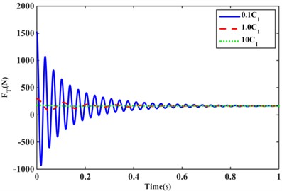
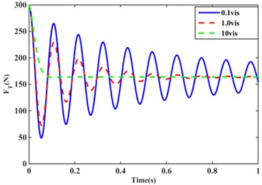
The upper chamber compliance $C_{1}$ of model I was varied in order to study the effect of the variation of $C_{1}$ on the hydraulic mount. The value of $C_{1}$ varies from 0.1 $C_{1}$ to 10 $C_{1}$ , and the variation of the hydraulic mount transfer force is shown in Fig. 7(a). When changing the compliance of the hydraulic mount upper chamber of model I to 0.1 $C_{1}$ , the amplitude of the transfer force increases significantly and the period decreases, as shown in the solid blue line in Fig. 7(a). Because according to Table 1 and Eq. (59), a decrease in $C_{1}$ leads to an increase in $λ$ , $ω_{n 2}$ . Similarly, when $C_{1}$ increases from 1.0 $C_{1}$ to 10 $C_{1}$ leads to a decrease in $λ$ and $ω_{n 2}$ , so the amplitude of the transfer force of the hydraulic mount of model 1 decreases significantly and the period increases for the same reason. When the viscosity vis is increased from 0.1 $v i s$ to 10 $v i s$ , it is clear from Fig. 7(b) that the transfer force of the hydraulic mount of model I gradually decreases, especially when increasing the fluid viscosity to 10 $v i s$ is the most obvious. This is due to the increase in viscosity $v i s$ leads to an increase in damping of the fluid flow through the inertia channel in Eq. (5), combined with the increase in $κ$ and $ς_{2}$ obtained from Table 1, and the decrease in the transfer force $F_{T} (t)$ of the hydraulic mount of model I according to Eq. (59).

Fig. 7Effect of upper chamber compliance and fluid viscosity on hydraulic mount transfer force: a) different C1 values, b) different fluid vis

a)

b)

5.2. Effect of inertia channel and orifice flow channel parameters on hydraulic mount

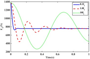
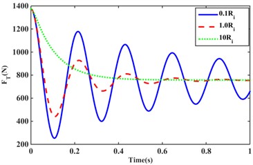
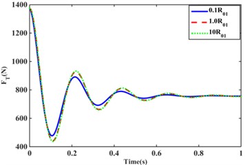
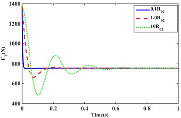
The effect of inertia and damping of the $Z_{4}$ structural inertia channel fluid of model II on the transfer force of the hydraulic mount under ideal step excitation is shown in Fig. 8(a), (b). As can be seen from Eq. (4), the value of $I_{i}$ is regulated by varying the length $L$ and effective cross-sectional area $A_{i}$ of the inertia channel, which has a significant effect on the peak and period of oscillation of the hydraulic mount under external excitation. Fig. 8(a) shows that as $I_{i}$ increases, the period of oscillation $t_{d} = 2 π / ω_{d}$ and the peak value of the transfer force increase. This is due to the combination of Table 1 and Eq. (75) increasing $I_{i}$ leads to a decrease in the rate of decay of the transfer force. As shown in Fig. 8(b), the step response of the hydraulic mount transfer force changes from an under-damped response to an over-damped response as the value of $R_{i}$ changes. At the same time, the increase in $R_{i}$ reduces the amplitude of the system oscillation, but the oscillation period $T_{d}$ increases slightly. Fig. 8(c), (d) shows the step response of the hydraulic mount transfer force by varying the damping values of the short flow channel of the $Z_{3}$ and $Z_{4}$ structures for the Model II configuration. Increasing the damping values $R_{01}$ and $R_{02}$ of the orifice flow channels $Z_{3}$ and $Z_{4}$ , the transfer force $F_{T} (t)$ oscillation increases. Instead, as the damping values $R_{01}$ and $R_{02}$ decrease, the transfer force $F_{T} (t)$ decays more rapidly. However, comparing Fig. 8(c) with Fig. 8(d) shows that the larger the cross-sectional area of the orifice flow channel the more rapidly the transfer force of the system decays.

5.3. Effect of different structural configurations on transfer force

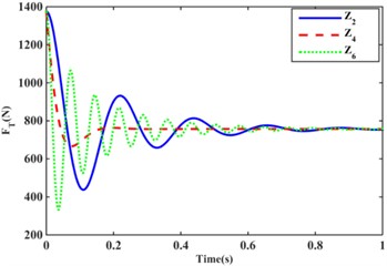
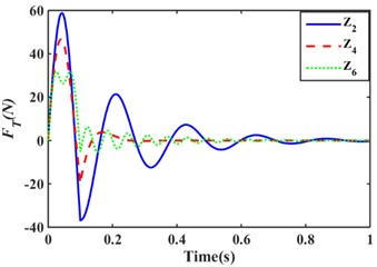
In order to compare the effects of different combinations of inertia channels and orifice flow channels on the performance of hydraulic mounts. Fig. 9 shows the variation of the transferred force for $Z_{2}$ in model 1 configuration, $Z_{4}$ in model 2 configuration and $Z_{6}$ in model 3 configuration for the same step excitation $x_{e} (t) = A_{1} u (t)$ and sinusoidal excitation $x_{e} (t) = A_{1} s i n (ω t)$ . It can be observed in Fig. 9 that the $Z_{4}$ structure in the model II configuration has the fastest decay of transfer force, followed by the $Z_{6}$ structure in the model III configuration, and the $Z_{2}$ structure in the model I configuration has the slowest decay of transfer force. As a result, it can be concluded that the presence of the orifice flow channel increases the damping of the system and minimizes the overshoot of the transfer force step response. Meanwhile, comparing the $Z_{2}$ and $Z_{6}$ structures, it can be found that although the $Z_{6}$ structure decays faster than the $Z_{2}$ structure, the oscillation period $T_{d}$ and the amount of overshoot of the $Z_{6}$ structure are significantly larger than those of the $Z_{2}$ structure.

Fig. 8Effect of model II hydraulic mount transfer force under ideal step excitation: a) inertia channel inertia; b) inertia channel damping; c) Z3 structural orifice flow channel damping; d) Z4 structural orifice flow channel damping

Effect of model II hydraulic mount transfer force under ideal step excitation: a) inertia channel inertia; b) inertia channel damping; c) Z3 structural orifice flow channel damping; d) Z4 structural orifice flow channel damping

a)

b)

c)

d)

Fig. 9Combination of hydraulic mounts with different inertia channels to transfer forces: a) step excitation; b) half sine excitation

a)

b)

6. Time-domain response analysis

6.1. Steady-state harmonic excitation response analysis

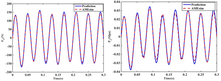
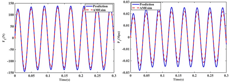
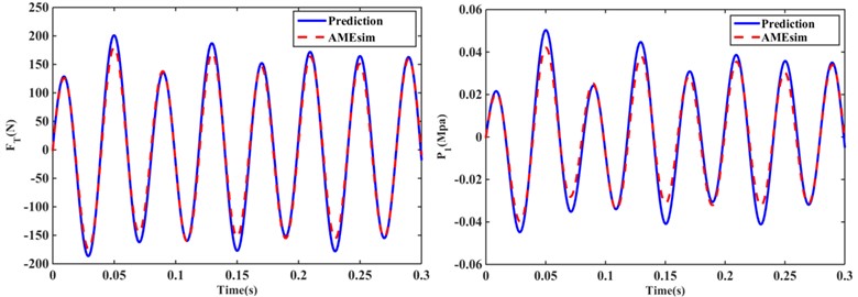
The blue line in Fig. 10 compares the response of the hydraulic mount transfer force and upper chamber pressure using the analytical solution of the steady-state response for Models I, II, and III solved in Section 3 with the red dashed line modeled using AMEsim. Fig. 10 show that the steady-state responses of the transfer force and upper chamber pressure solved using the analytical formula are in good agreement with the steady-state responses of the hydraulic mount solution built by AMEsim. For example, the errors between the RMS of the transfer force and the upper chamber pressure response solved by the two methods for the $Z_{1}$ the structure are 4.92 % and 9.81 %, respectively. The RMS of the transfer force and the pressure in the upper chamber of the $Z_{4}$ structure was 97.4724 N and 0.0178 MPa, respectively, when solved analytically, while the transfer force and the pressure in the upper chamber were 91.03 N and 0.01529 MPa when solved by AMEsim, with RMS errors of 6.61 % and 14.1 %. Similarly, the errors between the RMS of the transfer force and the upper chamber pressure response solved by the two methods for the $Z_{5}$ structure are 6.08 % and 10.81 %, respectively.

Fig. 10Steady-state response of transfer force and upper chamber pressure for Z1, Z4 and Z5 structures at 25 Hz, amplitude of 0.3 mm: a) Z1 structure; b) Z4 structure, c) Z5 structure

Steady-state response of transfer force and upper chamber pressure for Z1, Z4 and Z5 structures at 25 Hz, amplitude of 0.3 mm: a) Z1 structure; b) Z4 structure, c) Z5 structure

a)

b)

c)

6.2. Ideal step excitation response analysis

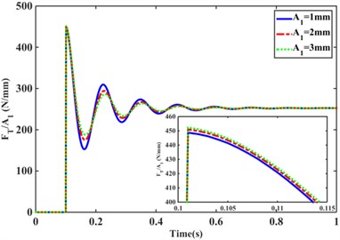
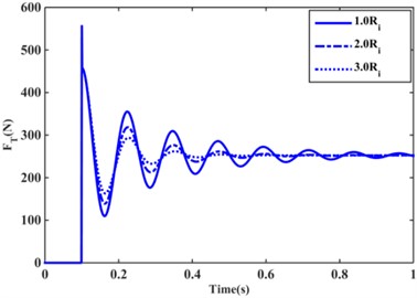
The transfer forces for the structure of Model 1 configuration at amplitudes $A_{1} =$ 1.0 mm, 2.0 mm, 3.0 mm are normalized and then overlapped in the same plot as shown in Fig. 11(a). From Fig. 11(a), it is observed that the overshoot of the transfer force decreases with the increase of the excitation amplitude and the transfer force decays faster while the oscillation period is longer. This means that as the excitation amplitude increases, the natural frequency and damping ratio of the system changes. To further illustrate whether the hydraulic mounts in the inertial channel configuration are damping related when the excitation amplitude varies leading to changes in the transfer force. The transfer force step response solved using the model 1 configuration $Z_{1}$ structure in Section III is shown in Fig. 11(b) by changing the damping value of the inertia channel from 1.0 $R_{i}$ to an increased value of 3.0 $R_{i}$ . Comparing Fig. 11(a), (b), it can be found that the damping of the inertial channel depends directly on the excitation amplitude. This conclusion is similar to that of reference studies on multi-inertia channel bushings [14].

Fig. 11Transfer force response of Z1 structure with different step excitation for model I configuration: a) Normalized response of transfer force with different excitation amplitude under AMEsim; b) Transfer force response with different damping values solved analytically

Transfer force response of Z1 structure with different step excitation for model I configuration: a) Normalized response of transfer force with different excitation amplitude under AMEsim; b) Transfer force response with different damping values solved analytically

a)

b)

7. Conclusions

The main contribution of the article is to investigate the time domain response of hydraulic mounts for the combination of long and short inertia channels and orifice flow channels since there are few studies on the time domain of hydraulic mounts for the combination of long and short inertia channels and orifice flow channels. A combination of numerical analysis and hydraulic analysis software AMEsim was used to compare the steady-state response and step response of different combinations of short and long inertia channels and orifice flow channels. Firstly, the transfer functions of dynamic stiffness and an upper chamber pressure of the hydraulic mounts of six configurations are derived using the lumped model. Secondly, the convolution method is used to solve the time domain analytic equations for the steady-state and step responses of the hydraulic mounts conFig.d in Model I, Model II, and Model III. Study shows that (1) increased compliance and fluid viscosity in the upper chamber of the hydraulic mount can rapidly decrease the transfer force; (2) Reducing the inertia of the inertia channel of the hydraulic mount and increasing the damping of the inertia channel can make the fastest transfer force reach the minimum value while increasing the cross-sectional area of the orifice flow channel can improve the damping value of the hydraulic mount. (3) The transfer forces and upper chamber pressures of the hydraulic mounts of different configurations obtained by the analytical method are in good agreement with the steady-state response of the mounts built by the hydraulic software AMEsim; (4) The effective damping is dependent on the excitation amplitude for hydraulic mounts.

References

Y. Yu, N. G. Naganathan, and R. V. Dukkipati, “A literature review of automotive vehicle engine mounting systems,” Mechanism and Machine Theory, Vol. 36, No. 1, pp. 123–142, Jan. 2001, https://doi.org/10.1016/s0094-114x(00)00023-9

Publisher
G. Kim and R. Singh, “A study of passive and adaptive hydraulic engine mount systems with emphasis on non-linear characteristics,” Journal of Sound and Vibration, Vol. 179, No. 3, pp. 427–453, Jan. 1995, https://doi.org/10.1006/jsvi.1995.0028

Publisher
Zhaoxue Deng, Qinghua Yang, and Xuejiao Yang, “Optimal design and experimental evaluation of magneto-rheological mount applied to start/stop mode of vehicle powertrain,” Journal of Intelligent Material Systems and Structures, Vol. 31, No. 3, 2020.

Publisher
Fu-Long Xin, X. Bai, and Li-Jun Qian, “Principle, modeling, and control of a magnetorheological elastomer dynamic vibration absorber for powertrain mount systems of automobiles,” Journal of Intelligent Material Systems and Structures, Vol. 28, No. 16, pp. 2239–2254, 2017.

Publisher
B.-H. Lee and C.-W. Lee, “Model based feed-forward control of electromagnetic type active control engine-mount system,” Journal of Sound and Vibration, Vol. 323, No. 3-5, pp. 574–593, Jun. 2009, https://doi.org/10.1016/j.jsv.2009.01.033

Publisher
R. Singh, G. Kim, and P. V. Ravindra, “Linear analysis of automotive hydro-mechanical mount with emphasis on decoupler characteristics,” Journal of Sound and Vibration, Vol. 158, No. 2, pp. 219–243, Oct. 1992, https://doi.org/10.1016/0022-460x(92)90047-2

Publisher
M. Tiwari, H. Adiguna, and Rajendra Singh, “Experimental characterization of a nonlinear hydraulic engine mount,” Noise Control Engineering Journal, Vol. 51, No. 1, pp. 212–223, 2003.

Publisher
Jong-Yun Yoon and Rajendra Singh, “Dynamic force transmitted by hydraulic mount: Estimation in frequency domain using motion and/or pressure measurements and quasi-linear models,” Noise Control Engineering Journal, Vol. 58, No. 4, 2010.

Publisher
J.-Y. Yoon and R. Singh, “Indirect measurement of dynamic force transmitted by a nonlinear hydraulic mount under sinusoidal excitation with focus on super-harmonics,” Journal of Sound and Vibration, Vol. 329, No. 25, pp. 5249–5272, Dec. 2010, https://doi.org/10.1016/j.jsv.2010.06.026

Publisher
F. Fallahi et al., “A modified design for hydraulic engine mount to improve its vibrational performance,” Proceedings of the Institution of Mechanical Engineers, Part C. Journal of Mechanical Engineering Science, Vol. 23, No. 23, 2021.

Publisher
X. Liao, X. Sun, and H. Wang, “Modeling and dynamic analysis of hydraulic damping rubber mount for cab under larger amplitude excitation,” Journal of Vibroengineering, Vol. 23, No. 3, pp. 542–558, May 2021, https://doi.org/10.21595/jve.2021.21921

Publisher
Y.-Q. Zhang and W.-B. Shangguan, “A novel approach for lower frequency performance design of hydraulic engine mounts,” Computers and Structures, Vol. 84, No. 8-9, pp. 572–584, Mar. 2006, https://doi.org/10.1016/j.compstruc.2005.11.001

Publisher
C. Yang et al., “Experiment and calculation of the low frequency performance of a hydraulic bushing with multiple tracks,” Journal of Vibration Measurement and Diagnosis, 2016.

Search CrossRef
C.-F. Yang, Z.-H. Yin, W.-B. Shangguan, and X.-C. Duan, “A study on the dynamic performance for hydraulically damped rubber bushings with multiple inertia tracks and orifices: parameter identification and modeling,” Shock and Vibration, Vol. 2016, pp. 1–16, 2016, https://doi.org/10.1155/2016/3695950

Publisher
T. Chai, J. T. Dreyer, and R. Singh, “Frequency domain properties of hydraulic bushing with long and short passages: System identification using theory and experiment,” Mechanical Systems and Signal Processing, Vol. 56-57, pp. 92–108, May 2015, https://doi.org/10.1016/j.ymssp.2014.11.003

Publisher
T. Chai, J. T. Dreyer, and R. Singh, “Time domain responses of hydraulic bushing with two flow passages,” Journal of Sound and Vibration, Vol. 333, No. 3, pp. 693–710, Feb. 2014, https://doi.org/10.1016/j.jsv.2013.09.037

Publisher
T. Chai, R. Singh, and J. Dreyer, “Dynamic stiffness of hydraulic bushing with multiple internal configurations,” SAE International Journal of Passenger Cars – Mechanical Systems, Vol. 6, No. 2, pp. 1209–1216, May 2013, https://doi.org/10.4271/2013-01-1924

Publisher
Lu M. and Ari-Gur J., “Study of hydromount and hydrobushing with multiple inertia tracks,” in JSAE Annual Congress Proceedings, 2002.

Search CrossRef
Y. Li, J. Z. Jiang, and S. A. Neild, “Optimal fluid passageway design methodology for hydraulic engine mounts considering both low and high frequency performances,” Journal of Vibration and Control, Vol. 25, No. 21-22, pp. 2749–2757, Nov. 2019, https://doi.org/10.1177/1077546319870036

Publisher
A. Shishegaran, H. Varaee, T. Rabczuk, and G. Shishegaran, “High correlated variables creator machine: Prediction of the compressive strength of concrete,” Computers and Structures, Vol. 247, p. 106479, Apr. 2021, https://doi.org/10.1016/j.compstruc.2021.106479

Publisher
A. Shishegaran, M. Saeedi, S. Mirvalad, and A. H. Korayem, “Computational predictions for estimating the performance of flexural and compressive strength of epoxy resin-based artificial stones,” Engineering with Computers, Vol. 39, No. 1, pp. 347–372, Feb. 2023, https://doi.org/10.1007/s00366-021-01560-y

Publisher
A. Shishegaran, M. R. Khalili, B. Karami, T. Rabczuk, and A. Shishegaran, “Computational predictions for estimating the maximum deflection of reinforced concrete panels subjected to the blast load,” International Journal of Impact Engineering, Vol. 139, p. 103527, May 2020, https://doi.org/10.1016/j.ijimpeng.2020.103527

Publisher
A. Shishegaran, A. N. Boushehri, and A. F. Ismail, “Gene expression programming for process parameter optimization during ultrafiltration of surfactant wastewater using hydrophilic polyethersulfone membrane,” Journal of Environmental Management, Vol. 264, p. 110444, Jun. 2020, https://doi.org/10.1016/j.jenvman.2020.110444

Publisher
B. Karami, A. Shishegaran, H. Taghavizade, and T. Rabczuk, “Presenting innovative ensemble model for prediction of the load carrying capacity of composite castellated steel beam under fire,” Structures, Vol. 33, pp. 4031–4052, Oct. 2021, https://doi.org/10.1016/j.istruc.2021.07.005

Publisher
M. A. Naghsh et al., “An innovative model for predicting the displacement and rotation of column-tree moment connection under fire,” Frontiers of Structural and Civil Engineering, Vol. 15, No. 1, pp. 194–212, Feb. 2021, https://doi.org/10.1007/s11709-020-0688-2

Publisher
A. Shishegaran, M. Saeedi, A. Kumar, and H. Ghiasinejad, “Prediction of air quality in Tehran by developing the nonlinear ensemble model,” Journal of Cleaner Production, Vol. 259, p. 120825, Jun. 2020, https://doi.org/10.1016/j.jclepro.2020.120825

Publisher
A. Shishegaran, M. Moradi, M. A. Naghsh, B. Karami, and A. Shishegaran, “Prediction of the load-carrying capacity of reinforced concrete connections under post-earthquake fire,” Journal of Zhejiang University-SCIENCE A, Vol. 22, No. 6, pp. 441–466, Jun. 2021, https://doi.org/10.1631/jzus.a2000268

Publisher
A. Shishegaran, B. Karami, E. Safari Danalou, H. Varaee, and T. Rabczuk, “Computational predictions for predicting the performance of steel 1 panel shear wall under explosive loads,” Engineering Computations, Vol. 38, No. 9, pp. 3564–3589, Sep. 2021, https://doi.org/10.1108/ec-09-2020-0492

Publisher
A. Shishegaran, M. Shokrollahi, A. Mirnorollahi, A. Shishegaran, and M. Mohammad Khani, “A novel ensemble model for predicting the performance of a novel vertical slot fishway,” Frontiers of Structural and Civil Engineering, Vol. 14, No. 6, pp. 1418–1444, Dec. 2020, https://doi.org/10.1007/s11709-020-0664-x

Publisher
A. Bigdeli, A. Shishegaran, M. A. Naghsh, B. Karami, A. Shishegaran, and G. Alizadeh, “Surrogate models for the prediction of damage in reinforced concrete tunnels under internal water pressure,” Journal of Zhejiang University-SCIENCE A, Vol. 22, No. 8, pp. 632–656, Aug. 2021, https://doi.org/10.1631/jzus.a2000290

Publisher
Yang C. F. et al., “Comparison of working mechanisms of hydraulic damped bushings and hydraulic engine mounts,” Journal of South China University of Technology (Natural Science Edition), 2015.

Search CrossRef
B. Barszcz, J. T. Dreyer, and R. Singh, “Experimental study of hydraulic engine mounts using multiple inertia tracks and orifices: Narrow and broad band tuning concepts,” Journal of Sound and Vibration, Vol. 331, No. 24, pp. 5209–5223, Nov. 2012, https://doi.org/10.1016/j.jsv.2012.07.001

Publisher
E. O. Doebelin, “System dynamics: modeling, analysis, simulation, design,” Marcel dekker, Inc, 1998.

Publisher
S. He and R. Singh, “Estimation of amplitude and frequency dependent parameters of hydraulic engine mount given limited dynamic stiffness measurements,” Noise Control Engineering Journal, Vol. 53, No. 6, pp. 271–285, 2005.

Publisher

About this article

Received

19 September 2022

Accepted

07 March 2023

Published

05 December 2023

SUBJECTS

Flow induced structural vibrations

DOI

https://doi.org/10.21595/jve.2023.22940

Keywords

long and short inertia channel; orifice flow channel; hydraulic mount; lumped parameters; transfer force

Acknowledgements

Science and Technology Guidance Project in Sanming City (2020-G-57), Fujian Province, China. China National Innovation and Entrepreneurship Training Program for college students (201911311010). Authors were supported by a grant from the Science and Technology Plan Project (2018Z016) of Quanzhou City, Fujian Province, China for the research in this paper. Sanming University introduced high-level talents scientific research start-up funding (Project number: 23YG01). Major Science and Technology Special Project of Fujian Province (2022HZ026025). Sanming science and technology plan project 2022-G-16. Fujian Province regional development project 2022H4009. Sanming University introduced high-level talents scientific research start-up funding (Project number: 23YG01). Sanming City Guiding Science and Technology Plan Project (Project Number: 2023-G-1).

Data Availability

The datasets generated during and/or analyzed during the current study are available from the corresponding author on reasonable request.

Author Contributions

Zhihong Lin – conceptualization, methodology, software, investigation, formal analysis, writing-original draft. Chunrong Wang – conceptualization, funding acquisition, writing-review and editing. Yunxiao Chen – software, validation. Mingzhong Wu – visualization, writing-review and editing. Feijie Zheng – software, validation. Jian Wei – visualization, writing-review and editing.

Conflict of interest

The authors declare that they have no conflict of interest.

This is an open access article distributed under the Creative Commons Attribution License, which permits unrestricted use, distribution, and reproduction in any medium, provided the original work is properly cited.

Previous article in issue Previous Next article in issue Next

Research article

2023 11 27

Analysis of the influence of the interaction between decoupled membrane channels and inertial channels on the mount' characteristics

Zhihong Lin, Yunxiao Chen, Mingzhong Wu, Feijie Zheng

Research article

2021 12 02

Simulation study about effects of fluid compressibility in hydraulic shock absorber based on AMEsim

Hailong Zou, Zhiyin Tang, Huijie Shen

Research article

2021 05 04

Modeling and dynamic analysis of hydraulic damping rubber mount for cab under larger amplitude excitation

Xin Liao, Xiaojuan Sun, Hu Wang

Research article

2020 04 02

Hydraulic damping nonlinearity of a compact hydro-pneumatic suspension considering gas-oil emulsion

Yuming Yin, Subhash Rakheja, Jue Yang, Alejandro Lozano-Guzman

Z. Lin, C. Wang, Y. Chen, M. Wu, F. Zheng, and J. Wei, “Time domain response analysis of multi-flow channel hydraulic mount,” Journal of Vibroengineering, Vol. 26, No. 1, pp. 152–173, Dec. 2023, https://doi.org/10.21595/jve.2023.22940

Copy Extrica

Copied to clipboard!

TY  - JOUR
DO  - 10.21595/jve.2023.22940
UR  - https://doi.org/10.21595/jve.2023.22940
TI  - Time domain response analysis of multi-flow channel hydraulic mount
T2  - Journal of Vibroengineering
AU  - Lin, Zhihong
AU  - Wang, Chunrong
AU  - Chen, Yunxiao
AU  - Wu, Mingzhong
AU  - Zheng, Feijie
AU  - Wei, Jian
PY  - 2023
DA  - 2023/12/05
PB  - Extrica
SP  - 152-173
VL  - 26
IS  - 1
SN  - 1392-8716
SN  - 2538-8460
ER  - 

Copy Ris

Copied to clipboard!

 @article{Lin_2023, title={Time domain response analysis of multi-flow channel hydraulic mount}, volume={26}, ISSN={2538-8460}, url={https://doi.org/10.21595/jve.2023.22940}, DOI={10.21595/jve.2023.22940}, number={1}, journal={Journal of Vibroengineering}, publisher={JVE International Ltd.}, author={Lin, Zhihong and Wang, Chunrong and Chen, Yunxiao and Wu, Mingzhong and Zheng, Feijie and Wei, Jian}, year={2023}, month=dec, pages={152–173} }

Copy Bibtex

Copied to clipboard!

[1]Z. Lin, C. Wang, Y. Chen, M. Wu, F. Zheng, and J. Wei, “Time domain response analysis of multi-flow channel hydraulic mount,” Journal of Vibroengineering, vol. 26, no. 1, pp. 152–173, Dec. 2023, doi: 10.21595/jve.2023.22940.

Copy IEEE

Copied to clipboard!

Lin, Zhihong, Chunrong Wang, Yunxiao Chen, Mingzhong Wu, Feijie Zheng, and Jian Wei. “Time Domain Response Analysis of Multi-Flow Channel Hydraulic Mount.” Journal of Vibroengineering 26, no. 1 (December 5, 2023): 152–73. https://doi.org/10.21595/jve.2023.22940.

Copy Chicago

Copied to clipboard!

Time domain response analysis of multi-flow channel hydraulic mount

Abstract

Highlights

1. Introduction

2. Hydraulic mount prototype study

2.1. Hydraulic mount structure

2.2. Hydraulic mount flow channel design with multiple configurations

2.3. AMEsim-based hydraulic mount study

3. Multi-flow channel hydraulic mount analysis model

3.1. Model I single inertia channel hydraulic mount

3.2. Model II combined inertial channel and orifice flow channel hydraulic mount

3.3. Model III parallel combination of 3 flow channel hydraulic mount

4. Multi-fluid hydraulic mount time domain analytical formula

4.1. Time domain steady-state harmonic response

4.1.1. Model I hydraulic mount

4.1.2. Model II hydraulic mount

4.1.3. Model III hydraulic mount

4.2. Transient response of ideal step excitation

5. Effect of different parameters on hydraulic mount

5.1. Compliance of the upper chamber and the viscosity of the fluid

5.2. Effect of inertia channel and orifice flow channel parameters on hydraulic mount

5.3. Effect of different structural configurations on transfer force

6. Time-domain response analysis

6.1. Steady-state harmonic excitation response analysis

6.2. Ideal step excitation response analysis

7. Conclusions

References

About this article

Related Articles