Abstract
Target detection is an important problem in computer vision and has important research value in the fields of pedestrian tracking, license plate recognition, and unmanned vehicles [1].The Viola-Jones algorithm is used to detect frontal face images, which improves the speed of face detection by tens or hundreds of times while obtaining the same or even better accuracy, but for special and HOG captures local shape information better and has good invariance to both geometric and optical changes, SVM solves machine learning in small sample cases, but its feature descriptor acquisition process is complex and has high dimensionality, leading to poor real-time performance, and the support vector machine algorithm is difficult to implement for large-scale training samples, while the deep learning-based YOLOv5 target detection algorithm combines the advantages of Viola-Jones algorithm and HOG+SVM algorithm to make up for the shortcomings of the above two algorithms, which is not only very stable for occlusion and complex case processing, but also can be implemented for large regular training samples, but the accuracy of YOLOv5 for target detection is not ideal, and this paper adds SENet mechanism in YOLOv5, which can make the network better to learn the locations in the images that need attention. Therefore, this paper first introduces the traditional target detection algorithm, then introduces and analyzes the Yolov5 algorithm, and improves and optimizes it, and compares it with the traditional target detection algorithm, and the results show that the improved Yolov5 algorithm has better results for target detection.
Highlights
- This paper presents a detailed comparison of the traditional target detection algorithms: Viola-Jones and Hog+SVM algorithms, illustrating their advantages, disadvantages and algorithmic steps.
- In this paper, the structure and process of the traditional YOLOV5 algorithm is introduced in detail, and under the comparison of the traditional target detection algorithm, it is found that although it has great advantages, it still cannot do more optimal processing in the face of the complex detection environment.
- In this paper, SENet is introduced to improve the original YOLOV5 network based on the original YOLOV5 algorithm. After training, it is found that the YOLOV5 algorithm with SENet mechanism is significantly better than the original YOLOV5 algorithm in terms of accuracy and leakage detection rate, while maintaining the real-time nature of the original algorithm.
1. Introduction
In recent years, target detection has been widely used in the field of intelligent transportation, and its purpose is to detect and identify vehicles, pedestrians and other traffic scene target information in traffic scenes using image processing, pattern recognition, machine learning, and deep learning technologies to achieve the goal of intelligent transportation and automatic driving, but the process of detection is subject to a variety of interference, such as angle, occlusion, light intensity and other factors, which adds new challenges to However, the detection process is subject to various interference, such as angle, occlusion, light intensity, etc., which adds new challenges to target detection, so a suitable target detection algorithm is especially important.
Traditional target detection algorithms generally use Viola-Jones algorithm, HOG+SVM-based target detection algorithm and DPM algorithm, but the current traditional target detection algorithms and strategies have been difficult to meet the requirements of data processing in target detection in terms of efficiency, performance, speed and intelligence in all aspects, they are more complex to apply in actual engineering, slow training speed and low accuracy, and The false detection rate is high. Therefore, in the context of the rapid development of convolutional neural networks, deep learning-based target detection algorithms are applied with good practical significance, which can achieve the analysis and processing of data features by studying and imitating the cognitive ability of the brain and have powerful visual target detection capability, and become the mainstream algorithm for current target detection. In this paper, we firstly introduce and analyze the traditional target detection algorithm, secondly introduce the target detection framework represented by YOLOv5 algorithm, analyze the shortcomings of the YOLOv5-based target detection algorithm, and make improvement and optimization for it, and verify it by MATLAB simulation to show what advantages the optimized algorithm has, and finally conclude the paper.
2. Traditional target detection algorithms
2.1. Viola-Jones algorithm
In face detection, the Viola-Jones algorithm is a very classical algorithm, which was proposed at CVPR in 2001 and is widely used for its efficient and fast detection[2].The Viola-Jones face detection algorithm has been successful in real-time detection of faces, which first uses Haar features to describe face features and uses the feature matrix module integral to represent this face image; then it is trained with Adaboost algorithm to build a hierarchical classifier to directly match the matrix feature regions to quickly determine whether the image is a face or not[3]. The specific process is as follows.
(1) Candidate frame selection.
The V-J framework uses the simplest sliding window method (exhaustive window scanning), which has a training scale of 24×24 sliding windows.
(2) Haar feature extraction.
About Haar feature, it is commonly known as the difference between white pixel points and black pixel points, value = white – black, which is a texture feature.
1) V-J algorithm feature extraction rectangle block diagram.
Including three kinds of features, divided into two rectangle features, three rectangle features, diagonal features. The following figure (Fig. 1, 2) shows.
Fig. 1Two rectangular features
2) Accelerated computational features using integral graphs.
An integral map is characterized by the fact that any point in that image is equal to the sum of all pixels located in the upper left corner of that point, which can be seen as an integral, hence the term integral map.
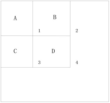
3) Calculating the sum of pixels within a square.
To understand how to calculate the pixel values within an arbitrary rectangle, we draw four regions A, B, C, and D and have four positions in the diagram as 1, 2, 3, and 4. The following diagram shows.
(3) Training face classifier.
V-J uses the Adaboost algorithm, which is based on the following principles.
a. Initialize the weights w of the samples, with the sum of the weights being 1.
b. Training the weak classifier.
c. Update the sample weights.
d. Repeat step b.
e. Finally combine the results of multiple weak classifiers for voting.
Combining multiple weak classifiers into one strong classifier is the core idea of the AdaBoost method.
Fig. 2Three rectangular features
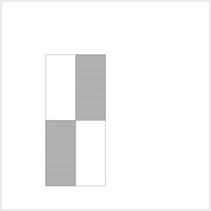
Fig. 3Hypothetical pixel location map
2.2. Hog+SVM algorithm
2.2.1. Hog algorithm
The HOG (Histogram of Oriented Gradient) feature detection algorithm, first proposed by French researcher Dalal et al. at CVPR-2005 [4], is a feature descriptor used for object detection in computer vision and image processing. The main idea is that the distribution of edge directions can also be a good representation of the profile contour of a pedestrian target when the specific location of the edge is unknown.
HOG feature algorithm flow:
(1) Color space normalization.
Due to the image acquisition environment, device and other factors, the effect of the acquired image may not be very good, and it is easy to have false detection or missed detection, so it is necessary to pre-process the acquired image. There are mainly two steps: graying out the image and Gamma correction.
a. Image grayscale.
The color image has R, G, B, 3 color channels, which are converted into a single-channel grayscale image:
b. Gamma correction.
In the case of uneven image brightness, Gamma correction can be used to increase or decrease the overall brightness in the image. The formula is as follows:
where is the weight value. Here we make 0.5, i.e., take the square root; you can also take other values by yourself to get different effects.
(2) Gradient calculation.
For the image after color space normalization, find its gradient and gradient direction. Calculated in the horizontal and vertical directions respectively, the gradient operator is:
(3) Gradient direction histogram.
The image is divided into several cels (cells), 8×8 = 64 pixels for a cell, no overlap between adjacent cells. In each cell, the histogram of gradient direction is counted, and all the gradient directions are divided into 9 bins (i.e. 9-dimensional feature vectors) as the horizontal axis of the histogram, and the cumulative value of the gradient values corresponding to the angle range as the vertical axis of the histogram.
(4) Overlapping block histogram normalization.
After normalizing the histogram of the overlapping blocks, the feature vectors of all blocks are combined to form a 26×37×36 = 34632-dimensional feature vector, which is the HOG feature, and this feature vector can be used to characterize the whole image.
The 330 3780-dimensional HOG features are used as test samples, and the support vector machine (SVM) classifier is used to discriminate whether there are pedestrians in the HOG features of these windows, and those with pedestrians are marked with rectangular boxes. We only need to get the HOG features and call SVM to get the discriminative result.
2.2.2. Principle of SVM algorithm
Support vector machines (SVM) is one of the most influential methods in supervised learning, and it is an algorithmic model proposed by the Soviet scholar Vapnik in solving pattern recognition problems [5]. Support vector machines are a binary classification model and the learning strategy of SVM is interval maximization, which can be formalized as a problem of solving convex quadratic programming, which is also equivalent to the problem of minimizing the loss function of a regularized hinge. the learning algorithm of SVM is the optimization algorithm for solving convex quadratic programming.
Input: training data set:
Among them:
Output: Separation of hyperplane and classification decision function
(1) Choose the penalty parameter 0, construct and solve the convex quadratic programming problem:
Obtain the optimal solution .
(2) Calculation choose . A component of satisfies the condition .
Calculation .
(3) Separation hyperplane , classification decision function:
2.2.3. HOG+SVM-based target detection algorithm flow
HOG features combined with SVM classifier have been widely used in image recognition, especially in pedestrian detection with great success. However, this model also needs to have a large number of positive and negative samples for training in order to improve the generalization ability of this model. The specific steps for its implementation are shown below [6].
Step 1. obtaining P blocks of positive samples from the training dataset and computing the HOG feature descriptors of these P blocks of positive samples.
Step 2. obtain N negative sample blocks from the training dataset and compute the HOG feature descriptors of these N negative sample blocks, where .
Step 3. train an SVM classifier model on top of these positive and negative sample blocks.
Step 4. apply hard-negative-mining. for each image in the negative training set and for each possible image scale, apply sliding windows on top of the images. Compute the corresponding HOG feature descriptors in each window and apply the classifier. If your classifier (incorrectly) classifies the given window as an object (it will definitely have false positives), record the feature vector associated with the false positive patch and the probability of classification. This method is called hard-negative-mining.
Step 5. first obtain the blocks of false positive samples obtained using the hard-negative-mining technique and then sort them according to their probability values; then retrain the classifier model using these blocks.
Step 6. applying the trained model to the test images.
Step 7. removing the redundant bboxes using NMS on the predicted results.
3. Traditional YOLOV5 algorithm
3.1. YOLOV5 network structure
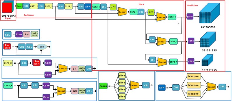
The following is a schematic diagram of the overall network structure of YOLOv5s [7].
The Fig. 4 shows the overall block diagram of the YOLOv4 target detection algorithm. For a target detection algorithm, we can usually divide it into four generic modules, specifically: the input, the reference network, the Neck network and the Head output, corresponding to the four red modules in the above Fig. 4 [8].
Fig. 4Yolov5 network structure
3.1.1. Input
The input side represents the input image. The input image size of this network is 608×608, and this stage usually contains an image preprocessing stage, which scales the input image to the input size of the network and performs operations such as normalization. Mosaic data enhancement is performed on the input image, and different images are stitched together by random scaling, random cropping, and random arrangement, and the Mosaic data enhancement method is used so that the images can not only enrich the background of the detection target, but also improve the detection of small targets [9]. Where Mosaic data enhancement probability is 1, which means it will definitely trigger, while Mix Up is not used for both small and nano versions of the model, and the other l/m/x series models use a probability of 0.1 to trigger Mix Up. small models have limited capability and generally do not use strong data enhancement strategies such as Mix Up.
The core Mosaic + Random Affine + Mix Up process is briefly mapped as follows.
Fig. 5Simple data enhancement process
Mosaic is a hybrid data enhancement, because it requires 4 images to be stitched together, which is equivalent to increasing the training batch size in disguise.
(1) Randomly generate the coordinates of the intersection center point of the 4 images after stitching, which is equivalent to determining the intersection point of the 4 stitched images.
(2) Randomly select the indexes of the other 3 images and read the corresponding annotations.
(3) Resize each image to the specified size by maintaining the aspect ratio.
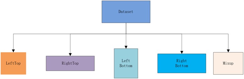
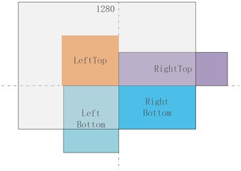
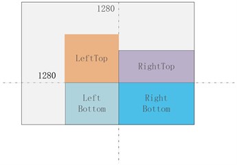
(4) Calculate the position of each image in the output image according to the rules of top, bottom, left and right, because the image may be out of bounds, so you also need to calculate the crop coordinates.
(5) Use the crop coordinates to crop the scaled image and paste it to the previously calculated position, and make up 114 pixels for the rest of the position.
(6) Process the label of each image accordingly.
Note: Since 4 images are stitched together, the output image area will be expanded by 4 times, from 640×640 to 1280×1280, so in order to revert to 640×640, we must add a RandomAffine random affine transformation, otherwise the image area will always be expanded by 4 times.
Fig. 6Hybrid data enhancement process
a) Embed image
b) Tailoring
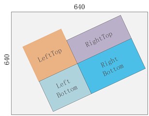
c) Affine transformation
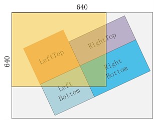
d) Image fusion
3.1.2. Backbone
Benchmark network-Benchmark network is usually a network of some high performance classifier species, and this module is used to extract some general feature representations.
The backbone network part is mainly used: Focus structure, CSP structure. Where Focus structure is not introduced in YOLOv1-YOLOv4, focus structure is introduced in YOLOv5 for direct processing of input images. Focus is important for slicing operation as shown below, 4×4×3 images are sliced into 2×2×12 feature maps [10].
The structure of YOLOv5s is that the original 608×608×3 image is input to the Focus structure, and a slicing operation is used to turn it into a 304×304×12 feature map first, and then a convolution operation with 32 convolution kernels to finally turn it into a 304×304×32 feature map.
3.1.3. Neck
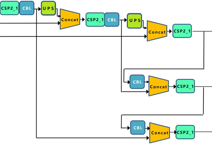
Neck network-Neck network is usually located in the middle of the benchmark network and the head network, and it can be utilized to further enhance the diversity and robustness of features. In the neck of the network, the following is used: FPN+PAN structure for rich feature fusion, FPN+PAN-YOLOv5s Neck network still uses the FPN+PAN structure, but some improvement operations are done on it. In the previous Neck structure of YOLO series algorithms, the ordinary convolution operations are used. In contrast, the CSP2 structure, which is borrowed from the CSPnet design, is used in the Neck network of YOLOv5, thus enhancing the network feature fusion capability [11].
(1) YOLOv5 not only replaces part of the CBL module using the CSP2_1 structure, but also removes the CBL module below it.
(2) The green area indicates the 2nd difference, where YOLOv5 not only replaces the CBL module after the Concat operation with the CSP2_1 module, but also replaces the position of the other CBL module.
(3) The blue area indicates the third difference, where YOLOv5 replaces the original CBL module with the CSP2_1 module.
Fig. 7Image transforms and slices
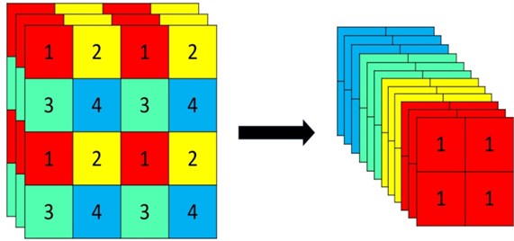
Fig. 8Neck network
3.1.4. Head
For the output of the network, following the consistent practice of the YOLO series, a coupled Head is used. and similar to YOLOv3 and YOLOv4, three different output Heads are used for multi-scale prediction. the loss function of the CIOU_Loss target detection task generally consists of two parts, the classification loss function and the regression loss function, and the development process of the regression loss function mainly include: the original Smooth L1 Loss function, the IOU Loss proposed in 2016, the GIOU Loss proposed in 2019, the DIOU Loss proposed in 2020 and the latest CIOU Loss function[12]-[15].
Fig. 9Loss function transformation
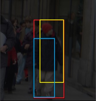
a) C: Minimum external rectangle
b) Difference set = C – parallel set B
The red box is the minimum outer rectangle (recorded as C), he is obtained from the mutual combination of the blue box and the yellow box, the yellow box represents the prediction box (recorded as B), the blue box represents the Ground truth box (recorded as A), C is the minimum outer rectangle of these two boxes, he added the intersection scale measurement, IOU is a common concept in vehicle target detection, is The higher the IOU, the stronger the object prediction accuracy. In Fig. 9, blue square A is the correct result of marking and yellow square B is the result predicted by the algorithm, then the IOU calculation formula is shown in Eq. (14). The loss function GIOU _Loss is calculated from the minimum outer rectangle C (as shown in Eq. (15)):
The meaning will be two arbitrary boxes A, B. We find a minimum closed shape C so that C can contain A, B. Then we calculate the ratio of the area in C that does not cover A and B to the total area of C. Then we subtract this ratio from the IoU of A and B. The CIOU_Loss of which is used in Yolov5 for the loss function of the Bounding box[16].
3.2. Shortcomings of YOLOv5 algorithm
The above analysis shows that although the YOLOv5s algorithm has the advantages of fast detection speed, high detection accuracy and lightweight model compared with other algorithms, it is still prone to the problem of wrong and missed detection when dealing with some complex background problems, thus revealing that the YOLOv5 algorithm has certain shortcomings.
(1) The YOLOv5 algorithm still has the phenomenon of missed detection for small targets and cohesive targets with mutual occlusion.
(2) The extraction of key feature information of the image is not perfect and sufficient.
In the process of extracting image features by the YOLOv5 algorithm, special attention is not given to the features in the image where the target information is particularly critical, and the irrelevant noise and the feature information that should be focused on cannot be distinguished and given different attention. For target detection, if this irrelevant noise information can be ignored and the important information can be focused on, it will be more beneficial to extract the key information of the target, so that better recognition can be achieved for the occluded images.
4. YOLO V5 algorithm optimization
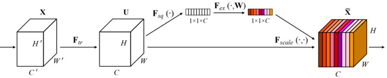
4.1. SENet attention mechanism
SENet is a typical implementation of the channel attention mechanism. SENet proposed in 2017 was the winner of the last ImageNet competition and its implementation is schematically shown below [17]. For the input incoming feature layer, we focus on its weights for each channel. For SENet, its focus is on getting the input incoming feature layer, the weights for each channel. Using SENet, we can make the network focus on the channels it needs to focus on the most. The specific implementation is as follows:
(1) Perform global average pooling for the feature layers coming in.
(2) Then two full connections are made, the first one with fewer neurons and the second one with the same number of neurons as the input feature layer.
(3) After completing two full connections, we take another Sigmoia to fix the value between 0 and 1. At this time, we obtain the weights of each channel (between 0 and 1) of the input feature layer.
(4) After obtaining this weight, we multiply this weight by the original input feature layer.
Fig. 10Schematic diagram of SENet mechanism implementation
4.2. YOLO v5 network improvement
In order to further improve the pedestrian detection effect in dense scenes, an improved YOLO V5 algorithm is proposed in the paper, which introduces the channel attention mechanism SENet to improve the backbone network of YOLO V5 and enhance the relevance representation of target information between different channels of the feature map, which can make the network pay more attention to the target to be detected and improve the detection efficiency. The structure of the YOLO V5 network after incorporating SE is shown in Fig. 11 (the red content in the figure is the structure of the incorporated SENet).
5. Simulation validation
5.1. Comparison of testing results
I have done a lot of experiments on several datasets, the effect is different for different datasets, and there are also differences in the methods for different additions to the same dataset, so you need to experiment. The majority of cases with effect and improvement.
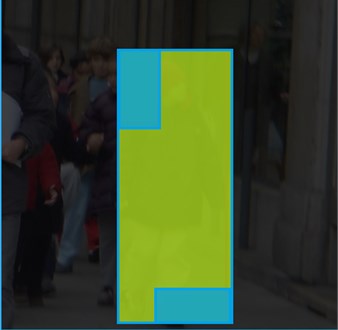
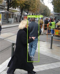
This training randomly selected 2 images from the complex pedestrian dataset as in Fig. 12(a) and Fig. 12(d) [18]. The detection was performed using the original YOLOv5 algorithm and the YOLOv5 algorithm with the addition of SENet, and the detection results are shown in Fig. 12(b), Fig. 12(c) and Fig. 12(e), and Fig. 12(f), respectively.
Fig. 11YOLOv5 algorithm with SENet mechanism
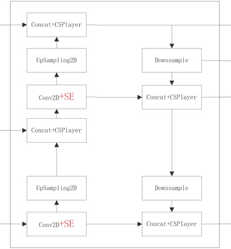
Fig. 12Comparison of the effect of the improved YOLOv5 algorithm with the unimproved algorithm of the original graph
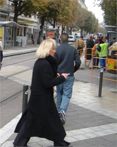
a) Original image
b) yolov5 algorithm detection
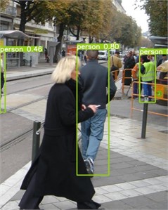
c) Detection after improved algorithm
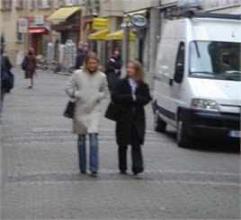
d) Original image
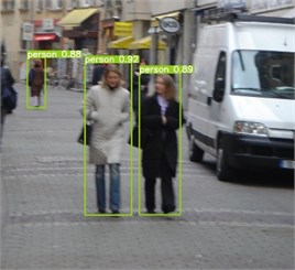
e) YOLOv5 algorithm detection
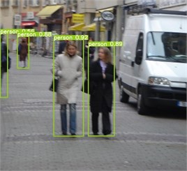
f) Detection after improved algorithm
Comparing with the above figure, it is clear that the improved algorithm with the addition of SENet only has an obvious advantage over the unimproved YOLOv5 algorithm in the face of obscured targets and distant targets detection, and after adding the attention mechanism of SE, the network is able to better learn the locations that need attention in the pictures, so the YOLOv5 algorithm with the addition of SENet is not disturbed by similar objects, and the SENet module effectively filters out the background interference in pedestrian detection, reducing the false detection rate and improving the detection accuracy.
5.2. Comparison of detection accuracy
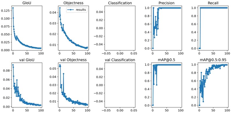
The training model and the graph of training parameters saved in the YOLOv5 folder under run after the training is completed.
Fig. 13Graph of training parameters
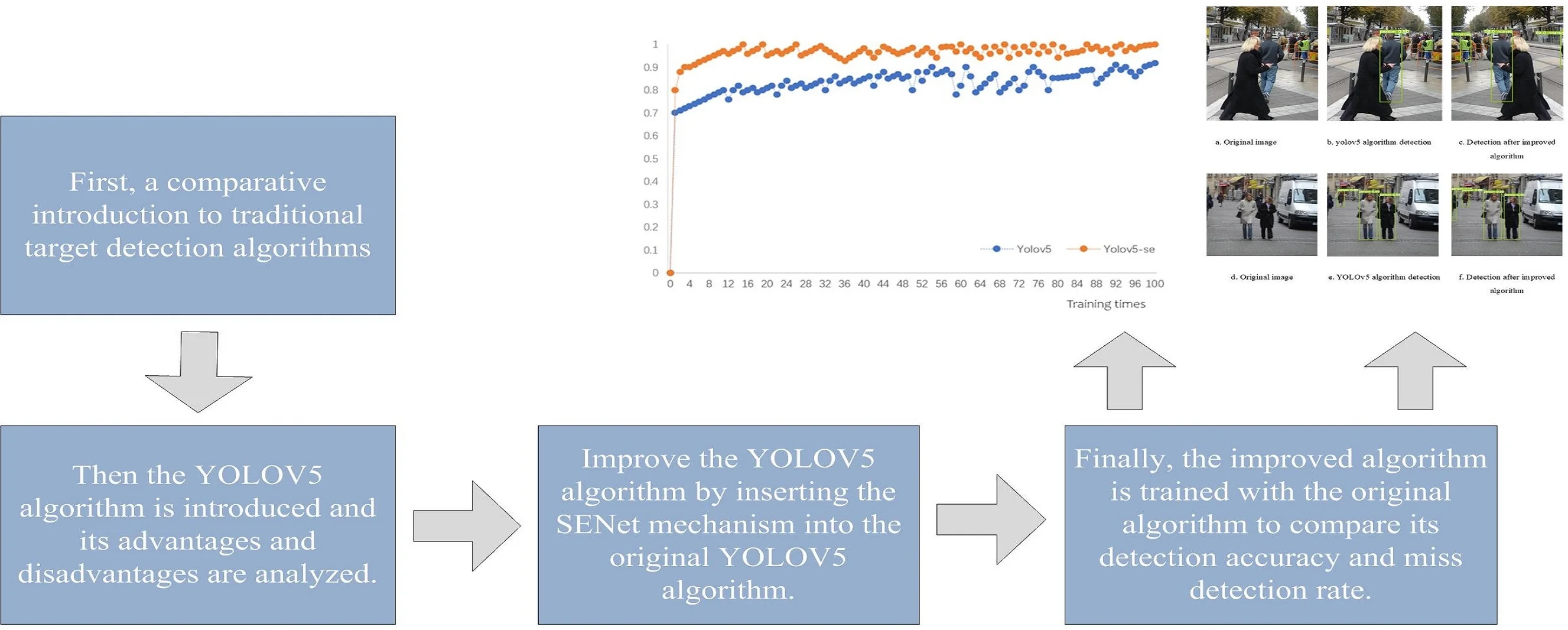
To be able to demonstrate the effectiveness of the optimized network, the paper compares the training times and the actual detection accuracy of the original YOLOv5 network and the YOLOv5 network with the addition of the SE attention mechanism in the same dataset. The convergence curves of the trained mAP are shown in Fig. 14, after training 100 times in the same dataset, respectively.
Fig. 14Comparison of the average accuracy values of the original YOLOv5 and the improved YOLOv5
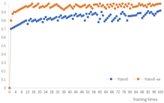
From the above figure, it can be seen that the accuracy rates of YOLOv5 and YOLOv5-SE networks change synchronously after 100 rounds of training on the dataset, and the accuracy rates converge to a stable level after 100 rounds of training. And after 100 rounds of training, the improved YOLOv5-se network after embedding SENet has higher accuracy than the original YOLOv5 model, which also indicates that the detection model after embedding SE mechanism has improved attention on target detection and helps to perform target recognition.
6. Conclusions
This paper mainly focuses on target detection based on YOLOv5 algorithm, and researches on YOLOv5 algorithm in target recognition algorithm, firstly introduces Viola-Jones algorithm and Hog+SVM algorithm, and addresses the problems such as incomplete recognition of small targets and mutually occluded targets when YOLOv5 algorithm performs target detection. In this paper, we propose an improved YOLOv5 algorithm by adding the SENet mechanism to the traditional YOLOV5 algorithm. Simulation results show that such improved algorithm performs significantly better than the traditional YOLOv5 algorithm in terms of target detection accuracy and miss detection rate, and also has the advantages of the traditional algorithm in real time, which meets the requirements of high speed and high accuracy when detecting pedestrians in complex scenes.
References
-
J. Wang, Y. Chen, S. Hao, X. Peng, and L. Hu, “Deep learning for sensor-based activity recognition: A survey,” Pattern Recognition Letters, Vol. 119, pp. 3–11, Mar. 2019, https://doi.org/10.1016/j.patrec.2018.02.010
-
M. Da’San, A. Alqudah, and O. Debeir, “Face detection using Viola and Jones method and neural networks,” in 2015 International Conference on Information and Communication Technology Research (ICTRC), pp. 40–43, May 2015, https://doi.org/10.1109/ictrc.2015.7156416
-
A. W. Y. Wai, S. M. Tahir, and Y. C. Chang, “GPU acceleration of real time Viola-Jones face detection,” in 2015 IEEE International Conference on Control System, Computing and Engineering (ICCSCE), pp. 183–188, Nov. 2015, https://doi.org/10.1109/iccsce.2015.7482181
-
N. Dalal and B. Triggs, “Histograms of oriented gradients for human detection,” in IEEE Computer Society Conference on Computer Vision and Pattern Recognition (CVPR’05), pp. 886–893, 2005, https://doi.org/10.1109/cvpr.2005.177
-
X. Liu, J. Xu, M. Li, and J. Peng, “Sensitivity analysis based SVM Application on automatic incident detection of rural road in China,” Mathematical Problems in Engineering, Vol. 2018, pp. 1–9, 2018, https://doi.org/10.1155/2018/9583285
-
P. Tribaldos, J. Serrano-Cuerda, M. T. López, A. Fernández-Caballero, and R. J. López-Sastre, “People detection in color and infrared video using HOG and linear SVM,” in Natural and Artificial Computation in Engineering and Medical Applications, pp. 179–189, 2013, https://doi.org/10.1007/978-3-642-38622-0_19
-
L. Li, M. Liu, L. Sun, Y. Li, and N. Li, “ET-YOLOv5s: toward deep identification of students’ in-class behaviors,” IEEE Access, Vol. 10, pp. 44200–44211, 2022, https://doi.org/10.1109/access.2022.3169586
-
S. Li, Y. Li, Y. Li, M. Li, and X. Xu, “YOLO-FIRI: improved YOLOv5 for infrared image object detection,” IEEE Access, Vol. 9, pp. 141861–141875, 2021, https://doi.org/10.1109/access.2021.3120870
-
J. Chu, Z. Guo, and L. Leng, “Object detection based on multi-layer convolution feature fusion and online hard example mining,” IEEE Access, Vol. 6, pp. 19959–19967, 2018, https://doi.org/10.1109/access.2018.2815149
-
Z. Li, C. Peng, G. Yu, X. Zhang, Y. Deng, and J. Sun, “DetNet: design backbone for object detection,” in Computer Vision – ECCV 2018, pp. 339–354, 2018, https://doi.org/10.1007/978-3-030-01240-3_21
-
T.-Y. Lin, P. Dollar, R. Girshick, K. He, B. Hariharan, and S. Belongie, “Feature pyramid networks for object detection,” in 2017 IEEE Conference on Computer Vision and Pattern Recognition (CVPR), pp. 936–944, Jul. 2017, https://doi.org/10.1109/cvpr.2017.106
-
G. Synnaeve and E. Dupoux, “A temporal coherence loss function for learning unsupervised acoustic embeddings,” Procedia Computer Science, Vol. 81, pp. 95–100, 2016, https://doi.org/10.1016/j.procs.2016.04.035
-
D. Zhou et al., “IoU loss for 2D/3D object detection,” in 2019 International Conference on 3D Vision (3DV), pp. 85–94, Sep. 2019, https://doi.org/10.1109/3dv.2019.00019
-
H. Zhai, J. Cheng, and M. Wang, “Rethink the IoU-based loss functions for bounding box regression,” in 2020 IEEE 9th Joint International Information Technology and Artificial Intelligence Conference (ITAIC), pp. 1522–1528, Dec. 2020, https://doi.org/10.1109/itaic49862.2020.9339070
-
S. Du, B. Zhang, and P. Zhang, “Scale-sensitive IOU loss: an improved regression loss function in remote sensing object detection,” IEEE Access, Vol. 9, pp. 141258–141272, 2021, https://doi.org/10.1109/access.2021.3119562
-
H. Rezatofighi, N. Tsoi, J. Gwak, A. Sadeghian, I. Reid, and S. Savarese, “Generalized intersection over union: a metric and a loss for bounding box regression,” in 2019 IEEE/CVF Conference on Computer Vision and Pattern Recognition (CVPR), pp. 658–666, Jun. 2019, https://doi.org/10.1109/cvpr.2019.00075
-
D. Cheng, G. Meng, G. Cheng, and C. Pan, “SeNet: structured edge network for sea-land segmentation,” IEEE Geoscience and Remote Sensing Letters, Vol. 14, No. 2, pp. 247–251, Feb. 2017, https://doi.org/10.1109/lgrs.2016.2637439
-
N. J. Karthika and S. Chandran, “Addressing the false positives in pedestrian detection,” in Lecture Notes in Electrical Engineering, pp. 1083–1092, 2020, https://doi.org/10.1007/978-981-15-7031-5_103
Cited by
About this article

The authors have not disclosed any funding.
The datasets generated during and/or analyzed during the current study are available from the corresponding author on reasonable request.
ZhiZhan Lu provides the whole text idea, writing and optimization ideas. Wang Ruili makes key comments on the article. Jin Yunfeng makes key comments on the article. Liang Chao made constructive comments on the article, which were important for formatting and later revision
The authors declare that they have no conflict of interest.
