Abstract
Power equipment is an important component of the whole power system, so that it is obvious that it is required to develop a correct method for accurate analysis of the infrared image features of the equipment in the field of detection and recognition. This study proposes a troubleshooting strategy for the power equipment based on the improved AlexNet neural network. Multi-scale images based on the Pan model are used to determine the equipment features, and to determine the shortcomings of AlexNet neural network, such as slower recognition speed and easy overfitting. After knowing these shortcomings, it would become possible to improve the specific recognition model performance by adding a pooling layer, modifying the activation function, replacing the LRN with BN layer, and optimizing the parameters of the improved WOA algorithm, and other measures. In the simulation experiments, this paper's algorithm was compared with AlexNet, YOLO v3, and Faster R-CNN algorithms in the lightning arrester fault detection, circuit breaker fault detection, mutual transformer fault detection, and insulator fault detection improved by an average of 5.47 %, 4.69 %, and 3.42 %, which showed that the algorithm had a better recognition effect.

1. Introduction
It is obvious that power equipment is a key component of the power system, so its operating condition influences the operation of the entire power grid a lot. Due to the unpredictability of equipment failure, it brings great trouble to industrial production and people’s life, so it is extremely important to provide proper fault detection method in the field of current power equipment. At present, the equipment fault detection method mainly includes the signal diagnosis, sound diagnosis, infrared image diagnosis and other ways, and infrared image detection that can carried out with a time lag or in real time in the state of non-stop power. Despite this method is also fast and safe, requires no contact connections and is widely used in practice [1], this identification method is very susceptible to the interference of artificial factors, and the resulting image has such demerits as a poor resolution, low contrast, visual blurring and other shortcomings that affect the recognition accuracy. At present, the existing methods to solve the infrared image recognition method mainly focus on the technology improvement research [2-4] and segmentation technology research [5-7]. So, these methods can improve the recognition effect of infrared images, but these algorithms have a high degree of complexity, increasing the difficulty of image analysis and detection. With the development of information technology, the integration of artificial intelligence technology and image processing technology has become the main direction of current scholars' research [8]. Faster-RCNN and YOLO gained good results in fault identification of power equipment [9-12] and substantiated the positive effect of the application of artificial intelligence technology. AlexNet is a newer convolutional image recognition neural network model, that has a high recognition rate and other parameters, so it is widely used in agriculture, military, industry and other fields. Being especially actual in fault diagnosis of bearing equipment [13-14] and hydraulic piston pumps [15], AlexNet has a better effect than Faster-RCNN and YOLO. However, the infrared image diagnosis of power equipment is easily affected by the influence of temperature and light, resulting in the reduction of detection and recognition accuracy, so the AlexNet structure shall be installed in a protected space and shall be optimized in size. Based on the above two factors, the research proposes a fault diagnosis strategy for power equipment based on AlexNet neural network, so as to help electric power enterprises quickly find and remedy the faults of power equipment. This strategy provides as follows:
1) Adopts a multi-scale image input method for the different volumes, textures, structures and other characteristics of electric power equipment, and is able to solve the feature extraction of electric power equipment images in complex scenes such as extreme weather, light and so on.
2) Improves the recognition performance by adding a pooling layer, modifying the activation function, using the BN layer instead of LRN, and optimizing the model parameters using WOA algorithm in case of the shortcomings of AlexNet neural network structure, which has a slow recognition speed and is easy to overfitting.
In simulation experiments, this paper’s algorithm is compared with several current popular image recognition algorithms, such as optimized YOLO v3, optimized Faster-RCNN, and the results illustrate the recognition performance of this paper’s algorithm.
The structure applied in this paper is as follows: Section 2 describes the current research status of image recognition and fault diagnosis of power equipment, Section 3 describes the AlexNet model and WOA algorithm that need to be used in this paper, Section 4 describes the process of infrared image detection and recognition of power equipment based on the improvement of AlexNet; Section 5 conducts the simulation experiments to validate the recognition effect of this paper's algorithms with respect to the power equipment, and Section 6 concludes the whole paper.
2. Related works
Scholars have used three main AI techniques for fault detection of devices in their researches: CNN, YOLO and other AI techniques.
(1) CNN related technology research. Literature [9] uses improved the Faster R-CNN for infrared image target detection of electrical equipment in substations. Their simulation experiments illustrate that the improved measures have obvious effects to enhance the accuracy of target detection. Literature [10] enhances the proportion of residual blocks in the basic Faster R-CNN model, which makes the network’s ability to acquire features enhanced, and the experiments illustrate greater accuracy in terms of MAP metrics. Literature [16] proposes a deep learning-based power IoT device detection strategy, which mainly uses a multi-channel-based CNN fault detection method, and their experiments verify the effectiveness of the method. Literature [17] proposes a target detection model based on the important region recommendation network, which reduces the background interference by calculating the weight of the feature map, and their experiments show that the image detection algorithm has a certain degree of feasibility. Literature [18] proposes a visible light image recognition model for substation equipment based on the Mask R-CNN, which has good results in fault detection and recognition effects of 11 typical substation equipment. Literature [19] applies the Faster R-CNN algorithm for the equipment recognition and state detection in electric power plant rooms, and the mAP of all test images in the simulation experiments is 91.3 %, which further verifies that the algorithm has a recognition effect. Literature [20] combines a deep convolutional neural network model for power equipment remote sensing image target detection, and FTL-R-CNN neural network model to complete the detection and analysis of equipment targets in order to obtain, in terms of the actual test data, the high detection accuracy and confidence.
(2) YOLO related technology research. Literature [11] proposes a new method for power equipment fault detection based on YOLO v4, and simulation experiments illustrate that the effective intelligent diagnosis of faults is achieved through target identification and fast extraction of equipment temperature. Literature [21] proposed an improved YOLO v4 backbone network for solving the problem of difficult localization in target detection of power equipment, which greatly alleviates the problem of low detection accuracy due to the imbalance of positive and negative samples. Literature [22] uses a lightweight multilayer convolutional neural network based on YOLO v3 for a multi-fault diagnosis, and the experimental results show that the framework has a better recognition accuracy, which improves the performance of defect analysis applications. Literature [23] proposed an improved Yolo v3 algorithm to detect electrical connector defects, and the results show that the Yolo v3 algorithm has faster recognition speed compared to the Faster R-CNN.
(3) Other artificial intelligence techniques. Literature [12] proposes a multi-label image recognition model based on the multi-scale dynamic graph convolutional network for power equipment detection, and the experimental results are analyzed to show that the model improves the results by 0.8 % and 31.8 % compared to the original model and the baseline model, respectively. Literature [24] proposes a matching algorithm based on phase consistency and scale invariant features, which is able to solve the problem of dense and accurate matching of visible and infrared images in power equipment.
These research results show that CNN and YOLO-based neural network models have a certain effect in power equipment fault detection, but the CNN correlation model of its own structure is relatively complex, and at the same time, it is inconsistent to process models of different sizes and target proportions, because it can easily lead to the identification of infrared images of different power equipment with a greater error risk, the YOLO correlation model in the processing of large-scale infrared images of electric power equipment has a better effect, but this model is not precise enough for the detection of small targets, and, at the same time, in case of the occlusion or availability irregularly shaped equipment, the results can be inaccurate.
In this paper, the AlexNet model is introduced in the power equipment fault detection, because this model pioneers the application of deep convolutional neural networks in computer vision tasks, has a higher accuracy for image recognition, improves the model's recognition ability by using more convolutional and fully-connected layers, helps to alleviate the problem of gradient vanishing, and has better recognition results than the current CNN and YOLO models. The recognition effect is better than the current CNN and YOLO models. Meanwhile, the AlexNet model was improved in this paper by optimizing the number of convolutional layers, pooling layers, modifying the activation function, and optimizing the important parameters using the whale optimization algorithm to improve the diagnostic performance of the AlexNet model.
3. Basic algorithms
3.1. AlexNet
AlexNet is a deep convolutional neural network model proposed by Alex Krizhevsky et al. in [25], which made a remarkable breakthrough in the ImageNet image classification challenge. AlexNet uses a deep convolutional neural network structure, which consists of five convolutional layers, three fully connected layers, and a final output layer. The structure is shown in Fig. 1.
Fig. 1AlexNet structure
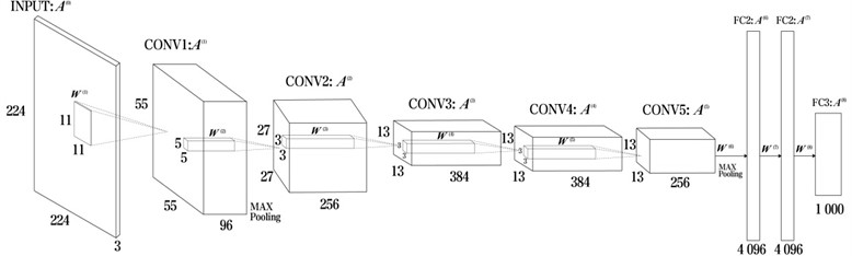
The main features of AlexNet are as follows:
(1) Alternating stacks of convolutional and pooling layers: the first 5 layers of AlexNet are alternating stacks of convolutional and pooling layers. The first convolutional layer uses 96 filters of size 11×11 with a step size of 4. Subsequent convolutional layers use smaller filters (size 5×5 or 3×3) but with more channels. The pooling layer uses the maximum pooling for downsampling to reduce the size of the feature map.
(2) ReLU nonlinear activation function: AlexNet uses a modified linear unit (ReLU) as an activation function to increase the nonlinear expressiveness of the network. The ReLU function perfectly handles the gradient vanishing problem and speeds up the computation.
(3) Local Response Normalization (LRN): after each convolutional layer, AlexNet introduces a local response normalization layer. This layer operation allows neurons with larger responses to get larger response values, thus improving the generalization ability of the network.
(4) Dropout regularization: AlexNet introduces the Dropout regularization technique to reduce overfitting between the fully connected layers. By randomly setting the output of some neurons to 0, Dropout can force the network to learn features that are more robust and have better generalization performance.
(5) Multi-GPU parallel training: AlexNet is the first deep learning model to fully utilize multiple GPUs for parallel training. By assigning different parts of the neural network to different GPUs and communicating and synchronizing between GPUs, AlexNet is able to accelerate the training process of the network and improve the performance.
AlexNet is a deep convolutional neural network model that successfully achieves the classification task on large-scale image datasets by using advanced techniques such as deep convolutional and pooling layers, ReLU activation function, LRN, Dropout, etc., which lays the foundation for the development of subsequent deep neural network models.
3.2. Whale optimization algorithm
Mirjalili S and Lewis A invented an intelligent optimization algorithm - Whale Optimization Algorithm based on the habits of whales, a large group of predators living in the oceans [26]. The algorithm carries out three main activities for prey, which are encircling predation, bubble attack and searching for prey. The size of the whole whale population is set as provided that the search algorithm space is -dimensional, and the position of the th whale in the -dimensional space is denoted as , , and the position where the whale captures the prey is the global optimal solution of the algorithm.
3.2.1. Surrounding predation
Whales use an encircling strategy to capture food in the sea, as well as the algorithm does in the beginning. The optimal position in the current group is assumed to be the current prey position, and then all other whales in the group swim towards the optimal position. The position of individual whales is updated according to Eq. (1):
where, denotes the position of the th whale individual in the th iteration, and denote the positions of the th and th whale individuals, respectively. is the enclosing step, and and are expressed as follows:
where, the algorithm is designed with two random parameters between (0, 1) and , which are used to control the parameters and . denotes the convergence factor, which controls the convergence of the algorithm, and is the maximum iteration result set by the algorithm.
3.2.2. Bubble attack
The whale optimization algorithm simulates the bubble attack behavior using shrink-wrapping and spiraling methods. Contraction envelopment is achieved through Eq. (2) and (4) as the convergence factor decreases. In spiral position updating, the individual whale obtains the distance to the current prey by calculating the distance between them and maintains the search for the prey in a spiral manner. Thus, the spiral wandering mode is formulated as follows:
where denotes the distance between the th whale and its prey in the th dimension of the spatial position update, denotes the limiting constant for the shape of the logarithmic spiral, and is a random number between –1 and 1. In particular, it is important to note that the probability of selection of the contraction-enclosure mechanism and the spiral position update is the same, and equal to 0.5.
3.2.3. Prey-seeking phase
Whales in the sea tend to search for food randomly, so the algorithms does as per the expression as follows:
where denotes the position of a randomly selected individual whale in the population at the current th iteration, and denotes the distance between a whale individual in the th dimension at each iteration and the current randomized individual.
It is well known that most of the parameters of deep learning models are set by human beings in a way that affects the model performance. So the use of meta-heuristic algorithms for optimizing the parameters of deep-learning models has been verified to be an effective method [27], and the literature [28-29] illustrates that the use of the WOA algorithm has a good performance in comparison with other meta-heuristic algorithms, and it has been widely used to obtain a better effect on optimizing the parameters of the deep-learning models.
4. Infrared image detection and recognition based on improved AlexNet neural networks
4.1. Multi-scale image processing
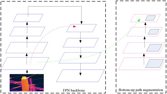
Traditional image recognition mainly extracts target features through layer-by-layer abstraction, in which the size of the sensory field of view is the key to obtaining target features. If the field of view is too small, only local features can be observed, and there is a possibility of losing the key information of the power equipment image; on the contrary, a lot of invalid information of the surrounding scene may be detected, which obstructs the correct infrared image feature extraction. The use of multi-scale image input enables the network to perceive the volume, texture, structure, etc. of power equipment at different scales, along with the impact of extreme weather, street buildings, light and other complex conditions which increase the difficulty of image extraction. The use of multi-scale image processing can accomplish better recognition results for power equipment targets at different distances. In this paper, the PAN model is applied [30] (Fig. 2) to obtain the image feature information, and utilize the bottom-up path technique of this model to increase the whole feature hierarchy, so as to obtain the image size features of different scales and improve the robustness of the model.
Fig. 2PAN model
4.2. Improved AlexNet model
Aiming at the shortcomings of AlexNet algorithm in image recognition, which is slow and prone to overfitting, the authors improve the model performance by reducing the number of convolutional layers, increasing the number of pooling layers, modifying the activation function, using the BN instead of LRU, and optimizing the weights and bias of AlexNet by using the whale optimization algorithm.
(1) Convolutional layers number reduction. The number of convolutional layers in the current AlexNet structure is 5 layers, which can effectively extract the deep features of infrared images of power equipment, but the deeper number of network layers leads to a long training time prone to overfitting. In this paper, a 3-layer convolutional neural network is used with 32 5×5 convolutional kernels in layer 1, 32 3×3 convolutional kernels in layer 2 and 64 5×5 convolutional kernels in layer 3, respectively. This setup can effectively maintain the number of convolutional layers, while reducing the problem of too deep layers, using a large number of convolutional kernels to complete the in-depth identification of image features, but still be able to maintain the ability to extract image features, and reduce the complexity of the model caused by the overfitting problem.
(2) Pooling layers number increase. Pooling layer is mainly used to reduce the size of the parameter matrix along with the reduction of other network parameters. Only one pooling layer is added after the second convolutional layer and the third convolutional layer of the AlexNet model, because the number of pooling layers is relatively small to avoid the loss of information and features, as well as to reduce the complexity of the model, improve the model invariance to spatial transformations, and reduce the sensory wildness of the network, which can reduce the risk of overfitting relatively.
(3) Activation function modification. The current AlexNet algorithm uses the ReLU activation function to solve the gradient disappearance and improve the convergence speed, but the neuron’s “death phenomenon” is easy to occur during the training process. As a result the neuron may no longer be activated by any data, so the network will not be able to perform the backpropagation and learning, then the ReLU function does not do amplitude compression of the data, resulting in the number of layers of the algorithm. As the ReLU function does not compress the data, the algorithm expands as the number of layers increases. In order to solve this problem, this paper chooses Leaky ReLU as the activation function, which can complete the backpropagation and solve the problem of gradient disappearance with the expression shown below:
where is a fixed slope, when 0, Leaky ReLU function can be back-propagated to solve the ReLU function neuron “death phenomenon”, and can solve the problem of gradient disappearance. However, because the value domain of Leaky ReLU activation function has no fixed interval, it is necessary to normalize the result of Leaky ReLU function with the expression as follows:
where is the normalized activation function value, denotes the output of the neuron at the th kernel location after its processing by the Leaky ReLU function, is the number of feature images, is the total number of feature image output channels, is the scaling factor, and is the exponential term.
(4) Exchange of LRN with BN layer. The parameter update of each layer in the inverse training process leads to changes in the input data distribution of the upper layer, which makes the deeper layer constantly re-adapt to the parameter update of the bottom layer, and the deeper the layer is, the more drastic the change in the parameter input distribution will be. Usually, in order to achieve better training results, a lower learning rate is often set, and saturation nonlinearity has to be avoided. In order to solve this problem, this study introduces the regularization layer of Batch Normalization (BN) [31] instead of LRN. The BN data normalization algorithm is shown in Eq. (9):
where denotes the input neurons, denotes the neuronal mean value of the training data elements, and denotes one standard deviation of the activation of the training data neuron . If only this normalization formula is used for a certain layer, it will reduce its expressive power, which in turn will affect the network’s ability to learn features. For this reason learnable parameters and are introduced for each neuron. The expression is as follows:
4.3. Improved whale optimization algorithm to optimize model parameters
Considering that the whale algorithm has low convergence accuracy and is easy to fall into the local optimum, this study further optimizes the performance of the algorithm from the population initialization and the dynamic division of the adaptive convergence factor.
4.3.1. Population initialization
Population initialization affects the convergence speed and accuracy of the algorithm, while the whale optimization algorithm only uses a random approach to initialization thus affecting the solution quality. The Laplace distribution function facilitates the exploration of the search space and the discovery of new potential solutions thus preventing the algorithm from falling into a local optimum. Therefore, the Laplace distribution is applied to generate the initial position of the individual whales. As a result of this action, the probability density function of the Laplace distribution will take the following form:
Therefore, the improved method of population initialization is as follows:
where is the Laplace distribution, is the location parameter, , are the scale parameters, , and the function is always symmetric with respect to the location parameter and is increasing on and decreasing on .
4.3.2. Adaptive factor optimization
In order to further improve the local search and global optimal ability of the traditional whale optimization algorithm, this paper optimizes the factor . The optimization expression is as follows:
where and denote the factor maximum and minimum values, respectively. In the early stage of the algorithm, due to a small value of , the whale individual approaches the global optimal individual slowly, which is favorable to the global search. In the middle and late stage of the algorithm, the value of gradually increases, the whale individual and the global optimal whale individual are located in the region close to each other, which is favorable to the local search, and maintains the diversity of the population. So the dynamics balances the algorithm's ability of the local search and the global optimal ability to avoid effectively the premature convergence phenomenon.
In order to better improve the recognition effect of AlexNet model in images, weights and bias being important components of the model performance, the parameter optimization is applied for the network model based on the whale optimization algorithm with the following steps:
Step 1: Define the objective function. Set the classification accuracy of AlexNet model as the objective function of whale optimization algorithm.
Step 2: Initialize whale individuals. Represent each whale individual as a set of neural network parameters.
Step 3: Calculate the fitness function. According to each whale individual, calculate the performance metric (classification accuracy) of the neural network as the fitness function of the individual.
Step 4: Update the global optimal solution. Select an individual whale with the highest fitness as the global optimal solution.
Step 5: Update whale position and velocity. For each whale individual, update the position and velocity of the whale based on the global optimal solution and the current optimal solution.
Step 6: Adjust the parameters. Update the weights and biases of the neural network by adjusting the parameter values of the individual whales.
Step 7: Iterative update: Repeat steps 3 to 6 until a preset stopping condition is reached, i.e. till the maximum number of iterations or the target accuracy rate.
Step 8: Output the optimal solution. Output the neural network parameter settings corresponding to the global optimal solution, i.e. as the best parameters of the optimized AlexNet neural network.
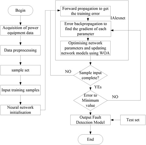
Therefore, the modified Alexnet power device is applied for infrared image detection process as shown in Fig. 3.
Fig. 3Flowchart of infrared image detection process
5. Simulation experiment
5.1. Performance comparison of whale optimization algorithm
In order to illustrate the performance of the improved whale optimization algorithm in this paper, the ACO algorithm, PSO algorithm, WOA algorithm and the algorithm of this paper-IWOA are selected for comparison. Table 1 shows six commonly used benchmark functions. Tables 2-7 show the comparison of the performance results of the four algorithms with the six benchmark functions. The maximum value, minimum value, variance and standard value are chosen as the measure of the performance comparison of the four algorithms.
Table 1Benchmark function
No. | Benchmark function | No. | Benchmark function |
F1 | F4 | ||
F2 | F5 | ||
F3 | F6 |
Based on the data provided in Tables 2-7, the IWOA clearly outperforms the other algorithms in terms of minimum, maximum, mean, and standard value results for the six functions studied. The superiority of IWOA compared to ACO and PSO is clearly demonstrated in these tables. In addition, the IWOA exhibits a clear performance advantage over the WOA, especially on functions F3, F5 and F6.
Table 2F1 test function comparison
Algorithm | Dim | Min value | Max value | Mean | St-deviation |
ACO | 2 | 2.3527 | 9.9684 | 4.2127 | 5.1629 |
5 | 5.8146 | 9.8915 | 8.1347 | 9.0442 | |
10 | 27.1343 | 100.1349 | 91.6176 | 75.1753 | |
30 | 87.1672 | 130.1363 | 97.1872 | 92.8172 | |
PSO | 2 | 2.9803 | 8.1257 | 5.0152 | 3.1258 |
5 | 9.0521 | 18.4956 | 11.2147 | 10.7517 | |
10 | 30.2918 | 100.4217 | 83.7527 | 78.9172 | |
30 | 90.8231 | 140.8162 | 128.7216 | 96.2952 | |
WOA | 2 | 9.1212E-04 | 3.9143E-02 | 3.1893E-03 | 5.2721E-03 |
5 | 4.8271E-08 | 7.9462E-07 | 3.2138E-06 | 2.1497E-06 | |
10 | 2.8314E-11 | 9.8752E-09 | 7.3912E-08 | 3.1271E-09 | |
30 | 7.5401E-15 | 2.6321E-10 | 2.3531E-11 | 3.5246E-12 | |
IWOA | 2 | 8.4012E-04 | 5.8917E-03 | 4.1029E-03 | 9.2731E-03 |
5 | 3.4412E-10 | 3.2348E-08 | 2.8426E-09 | 7.5421E-09 | |
10 | 4.1384E-14 | 2.6235E-10 | 5.1981E-11 | 4.1392E-09 | |
30 | 3.2187E-17 | 2.3681E-15 | 6.2982E-14 | 3.2741E-14 |
Table 3F2 test function comparison
Algorithm | Dim | Min value | Max value | Mean | St-deviation |
ACO | 2 | 2.3712 | 8.2318 | 4.8284 | 2.3531 |
5 | 10.1452 | 14.7229 | 12.1821 | 10.7842 | |
10 | 61.8391 | 79.2129 | 73.2126 | 72.1752 | |
30 | 90.8131 | 110.2315 | 95.3182 | 98.5315 | |
PSO | 2 | 5.5164 | 8.7018 | 6.2404 | 5.2156 |
5 | 8.6182 | 20.3721 | 16.9126 | 12.2973 | |
10 | 21.9102 | 53.2761 | 41.1831 | 48.5128 | |
30 | 80.1412 | 114.2691 | 86.3621 | 63.3914 | |
WOA | 2 | 8.1335E-03 | 3.3514E-01 | 8.1926E-02 | 3.8212E-03 |
5 | 9.1371E-04 | 7.9283E-02 | 4.9812E-01 | 3.1346E-02 | |
10 | 6.3174E-09 | 2.7416E-07 | 3.1238E-08 | 4.3128E-08 | |
30 | 3.3128E-15 | 9.9126E-10 | 3.8346E-11 | 3.7123E-12 | |
IWOA | 2 | 2.6125E-04 | 4.9193E-03 | 3.1597E-03 | 2.1839E-03 |
5 | 5.5915E-08 | 9.9143E-06 | 6.1929E-06 | 6.2612E-06 | |
10 | 1.4586E-18 | 1.1698E-16 | 1.1762E-16 | 1.1874E-16 | |
30 | 3.1982E-29 | 3.8485E-25 | 3.7043E-25 | 2.1466E-26 |
Table 4F3 test function comparison
Algorithm | Dim | Min value | Max value | Mean | St-deviation |
ACO | 2 | 1.9317 | 10.1894 | 9.4517 | 7.2465 |
5 | 3.3278 | 6.8219 | 6.7213 | 4.7813 | |
10 | 13.7813 | 27.6827 | 15.4322 | 15.7922 | |
30 | 29.3164 | 39.8264 | 32.9129 | 34.2154 | |
PSO | 2 | 4.1272 | 9.1045 | 6.2193 | 2.9108 |
5 | 8.1283 | 14.9134 | 12.3139 | 11.1418 | |
10 | 14.2164 | 61.1341 | 44.7542 | 43.6894 | |
30 | 64.9863 | 74.1284 | 70.1291 | 72.6354 | |
WOA | 2 | 6.7041E-04 | 1.922E-03 | 8.4612E-03 | 3.9254E-04 |
5 | 1.8817E-07 | 4.1691E-05 | 6.2134E-05 | 6.6745E-05 | |
10 | 1.3701E-15 | 3.5828E-10 | 6.1272E-08 | 3.7292E-09 | |
30 | 2.3146E-20 | 2.2214E-18 | 5.1249E-18 | 3.1214E-19 | |
IWOA | 2 | 0 | 3.3721E-04 | 2.1578E-04 | 5.3051E-04 |
5 | 9.1471E-08 | 5.1362E-06 | 2.5190E-06 | 7.1378E-06 | |
10 | 7.4471E-09 | 2.7805E-06 | 2.2801E-06 | 3.1874E-08 | |
30 | 3.3432E-26 | 5.9127E-25 | 5.6317E-24 | 9.8234E-24 |
Table 5F4 test function comparison
Algorithm | Dim | Min value | Max value | Mean | St-deviation |
ACO | 2 | 2.9172 | 6.1673 | 4.3278 | 4.2182 |
5 | 9.1423 | 13.3163 | 10.1783 | 9.1783 | |
10 | 19.1279 | 40.8122 | 24.1402 | 36.1953 | |
30 | 85.4056 | 99.3291 | 89.1736 | 91.2193 | |
PSO | 2 | 1.9032 | 3.7812 | 2.2196 | 2.6571 |
5 | 5.1085 | 10.3812 | 9.3717 | 7.6194 | |
10 | 15.8716 | 64.1218 | 36.8129 | 22.1975 | |
30 | 78.1476 | 126.71832 | 90.1472 | 69.1758 | |
WOA | 2 | 2.6512E-02 | 2.1925E+01 | 4.1643E-01 | 6.1254E-01 |
5 | 2.4061E-03 | 3.1029E+01 | 6.3218E-01 | 4.1927E+00 | |
10 | 9.0321E-07 | 6.1856E-03 | 4.2821E-03 | 3.1027E-04 | |
30 | 3.5712E-14 | 4.1235E-10 | 3.1738E-10 | 8.1525E-11 | |
IWOA | 2 | 4.1562E-04 | 1.0292E-03 | 5.8231E-03 | 3.1368E-03 |
5 | 4.5197E-07 | 3.8125E-06 | 5.8237E-06 | 4.1568E-05 | |
10 | 3.0165E-13 | 9.2815E-10 | 5.1275E-10 | 3.1428E-10 | |
30 | 1.5123E-16 | 1.239E-13 | 5.9201E-10 | 3.1563E-09 |
Table 6F5 test function comparison
Algorithm | Dim | Min value | Max value | Mean | St-deviation |
ACO | 2 | 2.2757 | 8.1365 | 6.1726 | 5.1538 |
5 | 5.1485 | 8.7219 | 5.9122 | 6.2178 | |
10 | 17.3176 | 40.9232 | 29.1956 | 33.1461 | |
30 | 40.9821 | 78.9341 | 54.9212 | 56.7216 | |
PSO | 2 | 5.6112 | 3.0152 | 3.1722 | 3.4732 |
5 | 8.1742 | 9.1213 | 3.1416 | 7.1565 | |
10 | 12.1877 | 15.1870 | 11.5714 | 14.8714 | |
30 | 38.0165 | 69.9267 | 40.1398 | 43.5813 | |
WOA | 2 | 4.9231E-05 | 8.1227E-03 | 6.1905E-04 | 1.5317E-05 |
5 | 3.3261E-05 | 3.1782E-02 | 5.1832E-03 | 5.8218E-03 | |
10 | 4.2521E-07 | 3.4713E-06 | 5.4316E-02 | 5.2174E-02 | |
30 | 3.8218E-11 | 1.8258E-08 | 4.1226E-09 | 4.089E-07 | |
IWOA | 2 | 6.1523E-06 | 6.1496E-04 | 6.1868E-05 | 3.1674E-05 |
5 | 5.5171E-10 | 0 | 3.1786E-07 | 6.2491E-07 | |
10 | 9.1058E-09 | 6.8673E-08 | 5.1574E-08 | 1.3143E-08 | |
30 | 3.8473E-13 | 9.0216E-10 | 5.2243E-10 | 3.7126E-10 |
Table 7F6 test function comparison
Algorithm | Dim | Min value | Max value | Mean | St-deviation |
ACO | 2 | 2.1296 | 7.4395 | 4.9365 | 6.2163 |
5 | 4.0289 | 9.4915 | 8.2932 | 5.8159 | |
10 | 10.2763 | 33.6967 | 28.6136 | 30.6732 | |
30 | 33.2593 | 74.2818 | 48.4178 | 48.1271 | |
PSO | 2 | 7.1795 | 8.9016 | 7.9315 | 3.1276 |
5 | 11.9821 | 13.0924 | 13.1043 | 13.9102 | |
10 | 4.9165E-03 | 3.0139E-02 | 3.9105E-03 | 3.9123E-03 | |
30 | 2.9724E-10 | 3.1376E-08 | 3.0987E-07 | 3.0159E-07 | |
WOA | 2 | 9.8132E-05 | 5.2154E-04 | 6.2712E-05 | 6.7821E-05 |
5 | 1.2461E-07 | 6.1357E-04 | 5.1762E-05 | 8.3931E-04 | |
10 | 7.7149E-10 | 4.1893E-09 | 4.6292E-07 | 5.2483E-05 | |
30 | 6.3127E-20 | 1.9193E-18 | 3.3126E-18 | 3.1923E-18 | |
IWOA | 2 | 0 | 1.5384E-04 | 5.8528E-05 | 3.3916E-04 |
5 | 5.7206E-07 | 3.6872E-05 | 3.3709E-05 | 4.8192E-05 | |
10 | 6.1882E-12 | 9.2913E-10 | 7.8716E-11 | 3.9127E-11 | |
30 | 6.6761E-24 | 1.7695E-20 | 4.8925E-21 | 3.9561E-21 |
It is noteworthy that IWOA has a minimum value of 0 when the dimensions are between 2 and 5, while the IWOA consistently provides favorable results on all six functions when the dimensions are between 10 and 30. This suggests that the overall performance of IWOA is greatly improved by strategies such as population initialization, call behavior optimization, and individual filtering. The consistently superior results obtained by IWOA on various statistical metrics, as well as its significant advantages over competing algorithms, validate the superiority of the population initialization, adaptive convergence factors, and dynamic partitioning employed in optimizing its overall performance.
5.2. Experimental comparison subjects
In order to verify that the algorithm (IAlexNet) in this paper has the effect, the AlexNet model, the YOLO v3 model from [13], and the Faster R-CNN model from [8] are selected for comparison. The Alexnet model is mainly composed of 5 convolutional layers, 3 maximum pooling layers, 3 FC layers using leaky ReLU activation function. YOLO v3 mainly uses DarkNet53 as the backbone network, 2 DBL units, 2 residual units and leaky ReLU activation function. Faster R-CNN uses VGG16 as the base model. Faster R-CNN uses VGG16 as the base model and leaky ReLU activation function. This study applies Tensorflow1.10.0 as an open source framework, Windows 10 as the operating system. The required hardware performance is: CPU of Core I7-6700, RAM of 16GB, and hard disk capacity of 1T. Fig. 4 shows the infrared images of some of the commonly used electric power devices.
Fig. 4Some commonly used electrical equipment
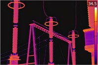
a) Surge arrester
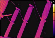
b) Circuit breakers
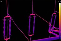
c) Transformers
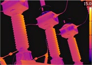
d) Insulators
5.3. Comparison of algorithm accuracy
In order to verify the performance of the algorithms in this paper, the accuracy values of the four algorithms we compared, and the results are shown in Fig. 5. The figure demonstrates that with the gradual increase in the number of training times, all the four algorithms show different degrees of upward trend in training accuracy values. When the number of training times reaches 400, the algorithm in this paper takes the lead in approaching stability and always maintains a flat state. While the AlexNet accuracy curve had an upward trend throughout the training process, the accuracy curves of YOLO v3 and Faster R-CNN algorithms also moved upward. Therefore, throughout the training process, the accuracy of this paper’s algorithm is better than the other three algorithms, indicating that this paper's algorithm has a more obvious improvement effect in AlexNet.
5.4. Comparison of algorithm effectiveness
This paper takes and considers 100 images of the above four power devices for verifying the algorithms performance. Table 8 shows the recognition results of the four algorithms for the four types of power equipment. From the results shown in the table, it is found that these algorithms have different results for the recognition rate of power equipment, but the advantage of this paper’s algorithm is more obvious. The color of the surrounding scene has a certain impact on the infrared image of the device, and the multi-scale image input of this paper’s algorithm reduces the impact of these invalid elements, thus making the device feature extraction more accurate. In a lightning arrester, the recognition rate of AlexNet, YOLO v3, Faster-RCNN increased by 6.54 %, 5.68 % and 3.95 %, respectively, in a circuit breaker, the recognition rate of AlexNet, YOLO v3, and Faster-RCNN is improved by 3.54 %, 3.47 % and 1.57 %, respectively. And finally, in mutual inductors, the recognition rate of AlexNet, YOLO v3, and Faster-RCNN is improved by 5.97 %, 4.94 % and 4.14 %, respectively, and in insulators, the recognition rate of AlexNet, YOLO v3, and Faster-RCNN is improved by 5.83 %, 4.67 %, and 4.38 %, respectively.
Fig. 5Comparison of training accuracy of four algorithms
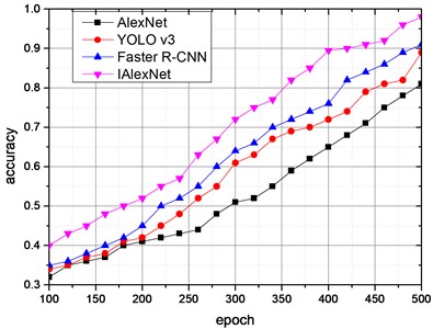
Table 8Comparison of the recognition effect of the contrasting algorithms in four kinds of electric equipment
Algorithm | Surge arrester | Circuit breakers | Transformers | Insulators |
AlexNet | 90.39 % | 91.93 % | 90.52 % | 90.83 % |
YOLO v3 | 91.13 % | 92.09 % | 91.41 % | 91.84 % |
Faster-RCNN | 92.65 % | 93.82 % | 92.12 % | 92.09 % |
IAlexNet | 96.31 % | 95.29 % | 95.93 % | 96.13 % |
Table 9 contains the recognition time comparison results for the four algorithms and four types of power equipment, and demonstrates that the IAlexNet algorithm applied in this paper has a clear advantage over AlexNet, and for YOLO v3, Faster -RCNN the advantage is even more dramatic. That substantiates such an optimization of the original AlexNet structure to improve the time complexity, decrease the recognition time.
Table 9Comparison of time consumed by contrasting algorithms in recognition of four types of power devices
Algorithm | Surge arrester (S) | Circuit breakers (S) | Transformers (S) | Insulators (S) |
AlexNet | 13.73 | 17.82 | 19.03 | 18.36 |
YOLO v3 | 13.67 | 16.79 | 18.94 | 18.27 |
Faster-RCNN | 13.28 | 16.84 | 18.96 | 18.28 |
IAlexNet | 13.26 | 16.85 | 18.94 | 18.32 |
Recall Rate (R) and Precision Rate (P) are the most important methods to measure the model recognition, in which Recall Rate (R) and Precision Rate (P) equations are as follows:
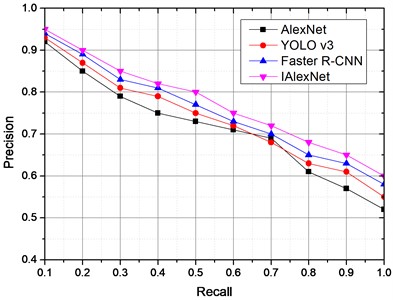
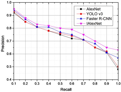
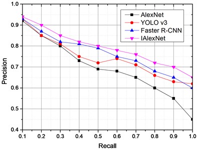
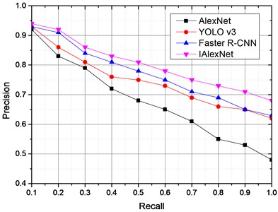
where, and denote the number of positive samples and negative samples being recognized correctly, respectively, denotes the number of positive samples being misclassified as negative samples, and denotes the number of all samples labeled as positive samples. In order to further verify the recognition effect of this paper’s algorithm before and after the improvement, the algorithm is optimized with or without SPP, with or without Leaky ReLU activation function, and with or without WOA in eight different conditions as shown in Table 10. Fig. 6 shows the PR results of this paper's algorithm with or without SPP, with or without Leaky ReLU activation function, and with or without WOA algorithm optimization for different algorithms in four kinds of power devices. From the results of the four devices, although the four algorithms show a downward trend, but the PR results of this paper’s algorithm has a more obvious advantage, which indicates at the increase of SPP, Leaky ReLU function and that the use of the WOA algorithm for the optimization of this paper’s algorithm is effective.
Table 10Classification of the main improvements of the algorithm in this paper
Case | SPP | Leaky ReLU | WOA |
case1 | NO | NO | NO |
case2 | NO | NO | YES |
case3 | NO | YES | YES |
case4 | NO | YES | NO |
case5 | YES | NO | NO |
case6 | YES | YES | NO |
case7 | YES | NO | YES |
case8 | YES | YES | YES |
Fig. 6PR values of four kinds of power devices which are the main improvement elements of this paper’s algorithm
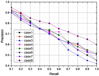
a) Surge arrester
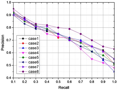
b) Circuit breakers
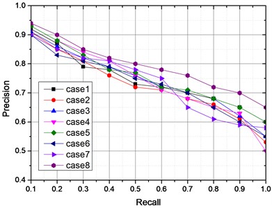
c) Transformers
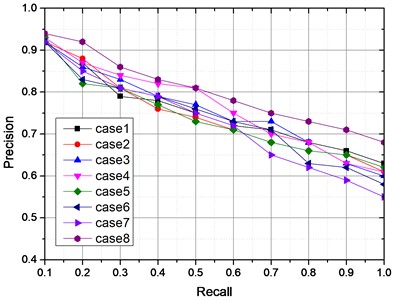
d) Insulators
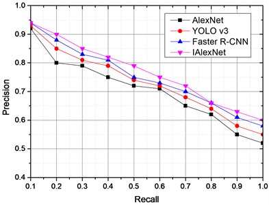
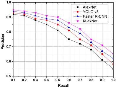
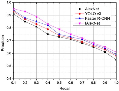
Fig. 7 shows the PR results of the four algorithms feature recognition, that explain that with the gradual increase in the R value, the four algorithms of the P value are in a gradual decline, and this paper algorithm R value in the range of [0, 0.6] is more gentle, compared to the other algorithms R value being equal to [0, 0.5], that demonstrates a more stable effect.
Fig. 7PRs of four power devices for four algorithms
a) Surge arrester
b) Circuit breakers
c) Transformers
d) Insulators
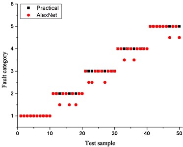
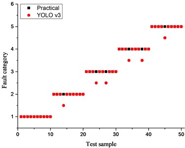
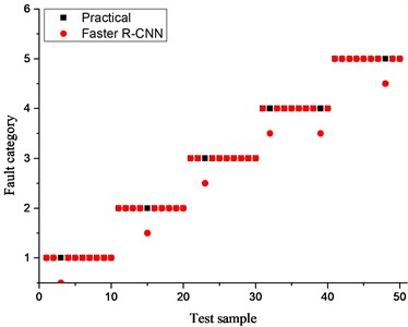
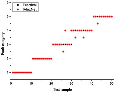
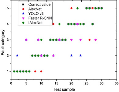
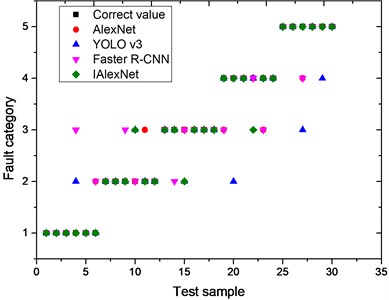
As per test diagnostic results of the four algorithms shown in Fig. 7, the mixed fault detection brings some detection difficulty to the model, compared to Fig. 6 having the categorized faults, where the fault identification samples during the detection process are more concentrated due to the troubleshooting in one device, and therefore the results can be obtained more accurately. The results of fault diagnosis shown in Fig. 7 (performed in the AlexNet model), three number 1 fault diagnosis results are wrong, two number 2 fault diagnosis results are wrong, number 3 fault diagnosis results are correct, three number 4 fault diagnosis results contain errors, two number 5 fault diagnosis also contain errors, and the comprehensive fault diagnosis success rate is 80 %. In the fault diagnosis using YOLO v3 model, two number 1 fault diagnosis results contain errors, two number 2 fault diagnosis results contain errors, number 3 faults all diagnosed correctly, one number 4 fault diagnosis contains an error, one number 5 fault diagnosis contains an error, the comprehensive fault diagnosis success rate is 88 %. In the Faster R-CNN model for fault diagnosis, one number 1 fault diagnosis result contains an error, two number 2 fault diagnosis results contain errors, 1 number 3 fault diagnosis, 1 number 4 fault diagnosis and 1 number 5 fault diagnosis results contain an error each, so the comprehensive fault diagnosis success rate is 88 %. And finally using the model in this paper for fault diagnosis, 1 number 1 fault diagnosis result contains an error, 2 number 2 fault diagnosis result contain errors, number 3 fault diagnosis and number 4 fault diagnosis results are all correct, 1 number 5 fault diagnosis contains an error, so the comprehensive fault diagnosis success rate is 92 %. From the above results, the four algorithms fault detection accuracy has been reduced, but the detection effect of the algorithm in this paper still has a certain advantage, and can better find the faults occurring in the power equipment.
To further illustrate the generality and robustness of the algorithms analyzed in this paper, the infrared images of power devices under different scenarios (Rainy day scenario, Hazy scenario, Cloudy scenario, and Sunny day scenario) we chosen for recognition. A mutual inductor was chosen as the research object, and its detection results from the four algorithms are shown in Fig. 8. From the detection results shown in Fig. 8, under four different scenarios, this paper’s algorithm still has a good PR value, and has better application results compared to the other three algorithms. Especially in the hazy day scenario, the PR values of the other three algorithms are significantly lower than those of this paper's algorithm. So the feature acquisition ability of the proposed model for images is significantly enhanced, and the performance of the model is improved by the optimization of the WOA algorithm.
Fig. 8PRs of four algorithms in different scenarios
a) Rainy day scenario
b) Hazy day scenario
c) Cloudy day scenario
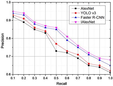
d) Sunny day scenario
5.5. Power equipment fault diagnosis
This subsection consists of the fault diagnosis of transformers, which are most frequently used in power equipment, as the object of study. At present, the faults of this type of equipment generally happen due to high-temperature overheating (for the sake of subsequent expression, the number is set to 1 and so on), low-temperature overheating (the number is set to 2), high-energy discharge (the number is set to 3), low-energy discharge (the number is set to 4), partial discharge (the number is set to 5), and normal state (the number is set to 6). Usually when a power transformer failure occurs, the device inside the transformer will dissolve hydrogen, methane, ethylene, acetylene and other gases, and the release of these gases captured by the infrared instrumentation gives the important information to determine the power transformer condition. A collection of 300 sets of power fault data from [32] is applied here. These 300 sets of data are distributed into the corresponding six categories of data based on the type of equipment failure. Among them, those numbered 1-50 belong to the number 1 faults, those numbered 61-100 belong to the number 2 faults, those numbered 101-150 belong to the number 3 faults, those numbered 151-200 belong to the number 4 faults, those numbered 201-250 belong to the number 5 faults, and those numbered 251-300 belong to the normal state of number 6. These data are also divided into a training set and a test set where 240 sets of sample data belong to the training set and 60 sets belong to the test set (the allocation results are shown in Table 11).
Table 11Sample training and test sets for six device states
1 | 2 | 3 | 4 | 5 | 6 | |
Training sample | 40 | 40 | 40 | 40 | 40 | 40 |
Test sample | 10 | 10 | 10 | 10 | 10 | 10 |
Table 12 shows the test results of the four algorithms in six equipment states, and these results explain that the recognition effect of this paper’s algorithm is obvious. For these six states of equipment faults, this paper’s algorithm improves the recognition rate by an average of 7 % compared to traditional AlexNet, and improves the recognition rate by an average of 4 % compared to YOLO v3 and Faster R-CNN, especially in the low-energy discharge faults, the algorithm of this paper has achieved 100 % recognition effect. These results demonstrate that the PAN-based model can effectively remove the interference influence around the device in image recognition. However, the AlexNet model has the advantages of increasing the pooling layer, modifying the activation function, using the BN layer instead of the LRN, and optimizing the model parameters using the WOA algorithm and other measures to improve the recognition performance of the model.
Table 12Test results of four algorithms in six device states
Algorithm | Fault Type | Number of trainings | Number of correct results | Accuracy |
AlexNet | 1 | 40 | 35 | 87.5 % |
2 | 40 | 36 | 90 % | |
3 | 40 | 34 | 85 % | |
4 | 40 | 35 | 87.5 % | |
5 | 40 | 34 | 85 % | |
6 | 40 | 35 | 87.5 % | |
YOLO v3 | 1 | 40 | 36 | 90 % |
2 | 40 | 37 | 92.5 % | |
3 | 40 | 35 | 87.5 % | |
4 | 40 | 36 | 90 % | |
5 | 40 | 37 | 92.5 % | |
6 | 40 | 36 | 93.3 % | |
Faster R-CNN | 1 | 40 | 36 | 86.7 % |
2 | 40 | 37 | 92.5 % | |
3 | 40 | 36 | 90 % | |
4 | 40 | 37 | 92.5 % | |
5 | 40 | 36 | 90 % | |
6 | 40 | 38 | 86.7 % | |
IAlexNet | 1 | 40 | 37 | 92.5 % |
2 | 40 | 38 | 95 % | |
3 | 40 | 39 | 97.5 % | |
4 | 40 | 40 | 100 % | |
5 | 40 | 38 | 95 % | |
6 | 40 | 39 | 97.5 % |
In order to further illustrate the effectiveness of the algorithmic aspects of this paper, this research authors selected 50 mixed test samples of different device faults (where 10 are selected for each non-normal state) and tested the four algorithms in comparison. The test results are shown in Fig. 9.
Fig. 9Fault diagnosis results for four algorithms
a) Alexnet troubleshooting results
b) YOLO v3 troubleshooting results
c) Fast R-CNN troubleshooting results
d) IAlexnet troubleshooting results
Fig. 10Fault diagnosis of two power substations
a) Paitou substation
b) Lizhu substation
In order to further illustrate the identification effect that the model in this paper has, the authors take the power equipment of Paitou Substation and Lizhu Substation under the jurisdiction of Shaoxing Branch of the State Electric Power Company, the author’s organization, as the practice object. Sample data of equipment records from January 2023 to May 2023 are collected. The authors selected a mixed test sample set of 30 transformer faults from each substation and compared them using four algorithms, and the results are shown in Fig. 10.
As per Fig. 10(a), the authors found that in the Pai Tau substation, the IAlexNet model has 4 errors, the traditional AlexNet model has 6 errors, YOLO v3 and Faster R-CNN have 7 errors, and as per Fig. 10(b), the IAlexNet model has 3 faults, the traditional AlexNet model has 5 errors, the YOLO v3 model has 6 errors, and the Faster R-CNN has 7 error faults. As per these results, the proposed algorithm has good results in the actual equipment detection process, and the detection success rate is close to 90 %.
6. Conclusions
Aiming at increasing the accuracy rate of the current infrared image fault diagnosis methods used for power equipment, the authors proposed an improved AlexNet-based fault diagnosis model and compared it with other methods traditionally applied for this purpose: AlexNet, YOLO v3 and Faster R-CNN. Furthermore, a PAN model, having the optimized AlexNet structure and other parameters, was introduced to obtain more accurate image features. The experimental results show that the proposed recognition algorithm has better results in power transformer troubleshooting. Nevertheless, the current improved AlexNet structure still has room for further optimization and can be a field of future research.
References
-
C. Xia et al., “Infrared thermography based diagnostics on power equipment: State-of-the-art,” High Voltage, Vol. 6, No. 3, pp. 387–407, Jul. 2021, https://doi.org/10.1049/hve2.120
-
A. S. N. Huda and S. Taib, “Application of infrared thermography for predictive/preventive maintenance of thermal defect in electrical equipment,” Applied Thermal Engineering, Vol. 61, No. 2, pp. 220–227, Nov. 2013, https://doi.org/10.1016/j.applthermaleng.2013.07.028
-
Y. Laib Dit Leksir, M. Mansour, and A. Moussaoui, “Localization of thermal anomalies in electrical equipment using infrared thermography and support vector machine,” Infrared Physics and Technology, Vol. 89, pp. 120–128, Mar. 2018, https://doi.org/10.1016/j.infrared.2017.12.015
-
X. Tan, X. Huang, C. Yin, S. Dadras, Y.-H. Cheng, and A. Shi, “Infrared detection method for hypervelocity impact based on thermal image fusion,” IEEE Access, Vol. 9, pp. 90510–90528, Jan. 2021, https://doi.org/10.1109/access.2021.3089007
-
C. Shanmugam and E. Chandira Sekaran, “IRT image segmentation and enhancement using FCM-MALO approach,” Infrared Physics and Technology, Vol. 97, pp. 187–196, Mar. 2019, https://doi.org/10.1016/j.infrared.2018.12.032
-
M. P. Manda, C. Park, B. Oh, and H.-S. Kim, “Marker-based watershed algorithm for segmentation of the infrared images,” in 2019 International SoC Design Conference (ISOCC), pp. 227–228, Oct. 2019, https://doi.org/10.1109/isocc47750.2019.9027721
-
D. Jha, M. A. Riegler, D. Johansen, P. Halvorsen, and H. D. Johansen, “DoubleU-net: a deep convolutional neural network for medical image segmentation,” in 2020 IEEE 33rd International Symposium on Computer-Based Medical Systems (CBMS), pp. 558–564, Jul. 2020, https://doi.org/10.1109/cbms49503.2020.00111
-
N. M. Nasrabadi, “Hyperspectral target detection: an overview of current and future challenges,” IEEE Signal Processing Magazine, Vol. 31, No. 1, pp. 34–44, Jan. 2014, https://doi.org/10.1109/msp.2013.2278992
-
J. Ou et al., “Infrared image target detection of substation electrical equipment using an improved faster R-CNN,” IEEE Transactions on Power Delivery, Vol. 38, No. 1, pp. 387–396, Feb. 2023, https://doi.org/10.1109/tpwrd.2022.3191694
-
T. Xue and C. Wu, “Target detection of substation electrical equipment from infrared images using an improved faster regions with convolutional neural network features algorithm,” Insight – Non-Destructive Testing and Condition Monitoring, Vol. 65, No. 8, pp. 423–432, Aug. 2023, https://doi.org/10.1784/insi.2023.65.8.423
-
H. Zheng, Y. Ping, Y. Cui, and J. Li, “Intelligent diagnosis method of power equipment faults based on single‐stage infrared image target detection,” IEEJ Transactions on Electrical and Electronic Engineering, Vol. 17, No. 12, pp. 1706–1716, Aug. 2022, https://doi.org/10.1002/tee.23681
-
Y. Yan, Y. Han, D. Qi, J. Lin, Z. Yang, and L. Jin, “Multi-label image recognition for electric power equipment inspection based on multi-scale dynamic graph convolution network,” Energy Reports, Vol. 9, pp. 1928–1937, Sep. 2023, https://doi.org/10.1016/j.egyr.2023.04.152
-
X. Shi et al., “An improved bearing fault diagnosis scheme based on hierarchical fuzzy entropy and Alexnet network,” IEEE Access, Vol. 9, pp. 61710–61720, Jan. 2021, https://doi.org/10.1109/access.2021.3073708
-
R. Ghulanavar, K. K. Dama, and A. Jagadeesh, “Diagnosis of faulty gears by modified AlexNet and improved grasshopper optimization algorithm (IGOA),” Journal of Mechanical Science and Technology, Vol. 34, No. 10, pp. 4173–4182, Oct. 2020, https://doi.org/10.1007/s12206-020-0909-6
-
Y. Zhu, G. Li, R. Wang, S. Tang, H. Su, and K. Cao, “Intelligent fault diagnosis of hydraulic piston pump based on wavelet analysis and improved Alexnet,” Sensors, Vol. 21, No. 2, p. 549, Jan. 2021, https://doi.org/10.3390/s21020549
-
R. Hou, M. Pan, Y. Zhao, and Y. Yang, “Image anomaly detection for IoT equipment based on deep learning,” Journal of Visual Communication and Image Representation, Vol. 64, p. 102599, Oct. 2019, https://doi.org/10.1016/j.jvcir.2019.102599
-
Y. Sun and Z. Yan, “Image target detection algorithm compression and pruning based on neural network,” Computer Science and Information Systems, Vol. 18, No. 2, pp. 499–516, Jan. 2021, https://doi.org/10.2298/csis200316007s
-
A. Jiang, N. Yan, F. Wang, H. Huang, H. Zhu, and B. Wei, “Visible image recognition of power transformer equipment based on mask R-CNN,” in 2019 IEEE Sustainable Power and Energy Conference (iSPEC), pp. 657–661, Nov. 2019, https://doi.org/10.1109/ispec48194.2019.8975213
-
Q. Zhang, X. Chang, Z. Meng, and Y. Li, “Equipment detection and recognition in electric power room based on faster R-CNN,” Procedia Computer Science, Vol. 183, pp. 324–330, Jan. 2021, https://doi.org/10.1016/j.procs.2021.02.066
-
H. Wang, H. Jiang, X. Liu, W. Yu, L. Yan, and S. Jin, “A remote sensing image based convolutional neural network for target detection of electric power,” in ICITEE2021: The 4th International Conference on Information Technologies and Electrical Engineering, pp. 1–6, Oct. 2021, https://doi.org/10.1145/3513142.3513207
-
X. Chen, Z. An, L. Huang, S. He, X. Zhang, and S. Lin, “Surface defect detection of electric power equipment in substation based on improved YOLOv4 algorithm,” in 2020 10th International Conference on Power and Energy Systems (ICPES), pp. 256–261, Dec. 2020, https://doi.org/10.1109/icpes51309.2020.9349721
-
W. Xia, J. Chen, W. Zheng, and H. Liu, “A multi-target detection based framework for defect analysis of electrical equipment,” in 2021 IEEE 6th International Conference on Cloud Computing and Big Data Analytics (ICCCBDA), pp. 483–487, Apr. 2021, https://doi.org/10.1109/icccbda51879.2021.9442579
-
W. Wu and Q. Li, “Machine vision inspection of electrical connectors based on improved Yolo v3,” IEEE Access, Vol. 8, pp. 166184–166196, Jan. 2020, https://doi.org/10.1109/access.2020.3022405
-
Z. Wang, X. Feng, G. Xu, and Y. Wu, “A robust visible and infrared image matching algorithm for power equipment based on phase congruency and scale-invariant feature,” Optics and Lasers in Engineering, Vol. 164, p. 107517, May 2023, https://doi.org/10.1016/j.optlaseng.2023.107517
-
A. Krizhevsky, I. Sutskever, and G. E. Hinton, “ImageNet classification with deep convolutional neural networks,” Communications of the ACM, Vol. 60, No. 6, pp. 84–90, May 2017, https://doi.org/10.1145/3065386
-
S. Mirjalili and A. Lewis, “The whale optimization algorithm,” Advances in Engineering Software, Vol. 95, pp. 51–67, May 2016, https://doi.org/10.1016/j.advengsoft.2016.01.008
-
H. Guo, J. Zhou, M. Koopialipoor, D. Jahed Armaghani, and M. M. Tahir, “Deep neural network and whale optimization algorithm to assess flyrock induced by blasting,” Engineering with Computers, Vol. 37, No. 1, pp. 173–186, Jul. 2019, https://doi.org/10.1007/s00366-019-00816-y
-
Y. Cui, S. Zhang, and Z. Zhang, “A parameter-optimized CNN using WOA and its application in fault diagnosis of bearing,” in 2023 IEEE 2nd International Conference on Electrical Engineering, Big Data and Algorithms (EEBDA), pp. 402–406, Feb. 2023, https://doi.org/10.1109/eebda56825.2023.10090663
-
M. E. Çimen and Y. Yalçın, “A novel hybrid firefly-whale optimization algorithm and its application to optimization of MPC parameters,” Soft Computing, Vol. 26, No. 4, pp. 1845–1872, Nov. 2021, https://doi.org/10.1007/s00500-021-06441-6
-
S. Liu, L. Qi, H. Qin, J. Shi, and J. Jia, “Path aggregation network for instance segmentation,” in 2018 IEEE/CVF Conference on Computer Vision and Pattern Recognition (CVPR), pp. 8759–8768, Jun. 2018, https://doi.org/10.1109/cvpr.2018.00913
-
S. Loffe and C. Szegedy, “Batch normalization: Accelerating deep network training by reducing internal covariate shift,” arXiv:1502.03167, pp. 448–456, Mar. 2015, https://doi.org/10.5555/3045118.3045167
-
X. F. Tian, “Research on transformer fault diagnosis based on improved bat algorithm optimized support vector machine,” (in Chinese), Heilongjiang Electric Power, Vol. 41, No. 1, pp. 11–15, 2019, https://doi.org/10.13625/j.cnki.hljep.2019.01.003
Cited by
About this article

The authors have not disclosed any funding.
The datasets generated during and/or analyzed during the current study are available from the corresponding author on reasonable request.
Fangheng Xu responsible for proposing the main modeling ideas and methods. Sha Liu is responsible for research and literature retrieval. Wen Zhang responsible for provides data related to power equipment.
The authors declare that they have no conflict of interest.
