Research on IGOA-LSSVM based fault diagnosis of power transformers

Power transformer is an important part of power equipment, and its functionality affects the proper operation of the whole power network. In order to diagnose power transformer faults effectively, the authors propose a fault diagnosis strategy based on an improved locust optimization algorithm for least squares vector machines (IGOA-LSSVM). Firstly, it was required to address the problem that the diagnostic prediction accuracy of the least squares vector machine is reduced due to its parameters. So this paper introduces the locust optimization algorithm with simple algorithm structure and good performance for optimizing the parameters. And at the same time, the authors generate an improved locust optimization algorithm with self-learning factors, proportional weight coefficients and Levy flight strategy. Secondly, the improved locust optimization algorithm is used for optimizing the least squares vector machine parameters. Finally, in the simulation experiments, the results of the benchmark test function illustrate that the IGOA algorithm has better performance, and the test results of a fault samples diagnosis of the power transformer equipment illustrate that the IGOA-LSSVM has good prediction effect and improves the fault identification accuracy compared with ACO-LSSVM and PSO-LSSVM in five types of fault diagnosis.

Research on IGOA-LSSVM based fault diagnosis of power transformers

1. Introduction

With the continuous improvement of national mechanization development level, the relationship between each equipment becomes intricate and complex, and the consequences brought by equipment failure will be unpredictable, so mechanical fault diagnosis technology has been highly valued by scholars. However, how to take accurate and efficient fault diagnosis method for mechanical equipment has been one of the first problems considered in the field of mechanical engineering. As the core component of the whole system, the power transformer equipment operates as an inseparable part of the whole power grid. Once the mechanical failure of the power transformer occurs, it will bring a great damage to the people as well as to the national property, so a research of power transformer is of the utmost importance. In this paper, the study is carried out from the perspective of transformer fault identification and diagnosis. Y. Sun et al. [1] proposed to use a BP neural network for a transformer fault diagnosis, through the neural network could effectively improve the fault. X. Yang et al. [2] proposed a neural network based on the BP-PNN for a transformer fault diagnosis, and proposed a dual fusion approach based on the BP and PNN for a fault feature identification, and then the simulation experiments showed that if used, the neural network had a better recognition effect. S. Fei et al. [3] proposed an identification idea consisting in optimizing the support vector machine based on the genetic algorithm, which was applied to optimize the parameters of support vector machine, thus improving the prediction performance of support vector machine. T. Kari et al. [4] proposed a hybrid feature selection method for power transformer fault diagnosis based on support vector machine and genetic algorithm, which had better results in extracting features. S. F. Cheng et al. [5] applied a wavelet neural network with improved particle swarm algorithm in transformer fault diagnosis, using the powerful ability of wavelet neural network to identify features for prediction, and optimizing wavelet neural network parameters using an improved particle swarm algorithm. Simulation experiments illustrated that the neural network had better results in transformer fault diagnosis. B. Zeng et al. [6] proposed to optimize a LSSVM neural network by using the wolf swarm algorithm, simulation experiments illustrated a significant improvement in fault feature recognition through the optimized LSSVM neural network. R. Naresh et al. [7] proposed an integrated neuro-fuzzy method for transformer fault diagnosis, which had a good effect for identifying transformer mechanical faults. L. Dong et al. [8] used a rough set and fuzzy wavelet neural network combined with the least squares weighted fusion algorithm in power transformer fault detection, which combined roughly set and wavelet neural fusion to improve the transformer fault diagnosis accuracy. P. Purkait et al. [9] proposed an expert system for transformer impulse fault diagnosis based on the time-frequency domain analysis, with the perspective to involve also the time frequency domain analysis to carry out the fault prediction study. D. Ma et al. [10] introduced an expert system for a fault diagnosis of power system based on a BP neural network, which mainly fuses multiple BP neural networks to predict and analyze the possible faults of power transformer equipment with the help of similar expert system, and the simulation experiment showed that the diagnosis system had a good effect. M. Demetgul et al. [11] proposed to use Gustafson-Kessel (GK) and k-medoids algorithm for fault clustering with an accuracy of about 90 %. Y. Miao et al. [12] proposed to use improved Blind deconvolution methods in fault diagnosis and described the prospects of application. W. Deng et al. [13] proposed a novel compound fault diagnosis method based on the optimized maximum correlation kurtosis deconvolution (MCKD) and sparse representation. The simulation experiments illustrated that the method allowed extracting the compound fault characteristics of rolling bearings and achieving accurate compound fault diagnosis. Q. Song et al. [14] proposed a multi-scale convolutional neural network (MSCNN) combined with a matrix diagram for chemical process fault diagnosis method, and simulation experiments illustrated that the algorithm had a good application perspective.

Having summarized the above literature research with different solutions to identify power transformer equipment faults, using neural networks to assist in equipment fault resolution, the authors of this paper determined the main direction that most scholars were still researching. But while the neural network parameter settings are the key factor for equipment diagnosis for this goal, combined with the basis of some scholars’ research, this paper proposes a locust optimization-based algorithm with a least squares vector machine optimization model, uses a locust algorithm to select the optimal parameter model, and finally applies the ready solution for the equipment fault diagnosis of power transformers. Simulation experiments illustrate that the diagnosis model has a good prediction effect.

2. Basic algorithm description

2.1. Grasshopper optimization algorithm

Saremi [15], an Australian scholar, proposed the Grasshopper optimization algorithm (GOA) based on the swarming behavior of Grasshoppers, which is divided into two parts, exploration and exploitation, where the exploration part corresponds to the larval stage of Grasshoppers and the exploitation part corresponds to the adult stage of Grasshoppers. In the larval stage, the Grasshoppers move to a small area, which is good for a local search. In the adult stage, Grasshoppers move to a small area, which facilitates a local search. The individual positions of Grasshopper populations are influenced by population interaction, gravitational forces and wind forces during reproduction, foraging and migration:

1

X_{i} = r_{1} S_{i} + r_{2} G_{i} + r_{3} A_{i},

where, $X_{i}$ denotes the position of the $i$ th Grasshopper, $S_{i}$ denotes the influence of the $i$ th Grasshopper by the interaction force of other Grasshoppers, $G_{i}$ is the influence of the $i$ th Grasshopper by the gravitational force, $A_{i}$ is the influence of the $i$ th Grasshopper by the wind force, and $r_{1}$ , $r_{2}$ , $r_{3}$ are random numbers which take the value of [0, 1], respectively, in the equation as follows:

2

S_{i} = \sum_{\begin{array}{l} j = 1 \\ j \neq i \end{array}}^{K} s (d_{i j}) {\hat{d}}_{i j},

where $K$ denotes the number of Grasshoppers, $d_{i j} = | x_{j} - x_{i} |$ denotes the distance between the $i$ , $j$ th of two Grasshoppers. ${\hat{d}}_{i j} = (x_{j} - x_{i}) / d_{i j}$ denotes the unit vector from $i$ Grasshopper to the $j$ th Grasshopper, and $s$ denotes the influence function between the Grasshoppers subjected to the interaction force with other Grasshoppers, expressed as follows:

3

s (r) = f e^{\frac{- r}{l}} - e^{- r} .

In Eq. (3), when $s (r)$ is greater than 0, Grasshoppers will attract each other, so the range of $r$ is called the attraction domain, when $s (r)$ is less than 0, Grasshoppers will repel each other, so the range of $r$ is called the repulsion domain; when $s (r)$ is 0, Grasshoppers will neither attract nor repel each other, so $r$ is the comfortable distance. In addition, $f$ and $l$ represent the attraction strength parameter and the scale parameter, respectively, and their values affect the domains of attraction, repulsion and moderate distribution distances, generally $l$ is 1.5 and $f$ is 0.5:

4

G_{r} = - g {\hat{e}}_{g},

5

A_{i} = u {\hat{e}}_{w} .

In Eq. (4), $g$ denotes the gravitational constant, ${\hat{e}}_{g}$ denotes the unit vector pointing at the center of the earth; in Eq. (5), $u$ denotes the wind direction constant, ${\hat{e}}_{w}$ denotes the wind direction unit vector, so the Grasshopper individual position is updated as follows:

6

X_{i} = \sum_{\begin{array}{l} j = 1 \\ j \neq i \end{array}}^{K} s (| x_{j} - x_{i} |) \frac{x_{j} - x_{i}}{d_{i j}} - g {\hat{e}}_{g} + u {\hat{e}}_{w} .

Although Eq. (6) is used to simulate the Grasshopper population, from the aspect of practical application, the gravitational factor is usually not considered, and the wind direction is determined to point at the target location, so the best individual Grasshopper location is solved as the optimization problem. The formula is shown below:

7

X_{i}^{d} = p \{\sum_{\begin{array}{l} j = 1 \\ j \neq i \end{array}}^{K} p \frac{u b_{d} - l b_{d}}{2} s (| x_{j}^{d} - x_{i}^{d} |) \frac{x_{j} - x_{i}}{d_{i j}}\} + {\hat{T}}_{d},

8

p = p_{m a x} - t \times \frac{p_{m a x} - p_{m i n}}{T_{m a x}},

where, $u b_{d}$ and $l b_{d}$ correspond to the upper and lower bounds of the $i$ th Grasshopper in the $d$ th dimension respectively, ${\hat{T}}_{d}$ is the target position of the Grasshopper swarm, $p$ in Eq. (8) is the decreasing coefficient, which is used to balance the global search and local exploitation ability on the one hand, and the exclusion and attraction domains on the other hand, $t$ is the number of current iterations, $p_{m a x}$ and $p_{m i n}$ are the maximum and minimum values respectively. $T_{m a x}$ is the maximum number of iterations

2.2. LSSVM

Least squares support vector machine (LSSVM) is a deformation algorithm for automatic vector machines that uses a least squares loss function instead of an insensitive loss function to convert the quadratic programming problem in automatic vector machine training into a set of linear equations solution problem, thus greatly reducing the complexity and speeding up the solution while ensuring the accuracy speed.

Let the training sample set for the binary classification problem be:

9

S = \{(x_{i}, y_{i}), x_{i} \in R^{n}, y_{i} \in \{- 1, + 1\}, i = 1,2, \dots n\},

where, $x_{i}$ denotes the $i$ th input sample, $y_{i}$ is the category label relative to $x_{i}$ , and $n$ is the number of samples. First, the samples to be classified are mapped to the high-dimensional space by introducing a nonlinear function, and then the optimal decision function is constructed in the high-dimensional space as follows:

10

f (x) = w^{t} φ (x) + b,

where, $w$ is the weight vector, $φ (x)$ is the mapping function, and $b$ is a constant, so the optimization function of the least squares vector machine is:

11

\begin{array}{l} \underset{ω, ξ, b}{m i n} \frac{1}{2} {‖ω‖}^{2} + c \frac{1}{2} \sum_{i = 1}^{M} ξ^{2}, \\ s . t . \\ {x'}_{l} = ω^{T} ϕ ({R^{'}}_{l}) + b + ξ_{l}, \end{array}

where, $ς$ is the relaxation variable, and $c$ is the regularization parameter.

The current LSSVM has many kernel functions, and its radial basis function has the advantages of parameters, generality, etc. In this paper, the authors choose it as the kernel function of LSSVM, which is determined as follows:

12

\begin{matrix} K ({R^{'}}_{m}, {R^{'}}_{n}) = e x p (\frac{- {‖{R^{'}}_{m}, {R^{'}}_{n}‖}^{2}}{2 σ^{2}}), (m, n = 1,2, . . ., M) . \end{matrix}

By introducing the Lagrange operators $a$ and $b$ , Eq. (11) is transformed into a pairwise problem, i.e.:

13

[\begin{array}{l} 0 & {\bar{1}}^{T} \\ \bar{1} & Ω + γ^{- 1} I \end{array}] [\begin{array}{l} b \\ a \end{array}] = [\begin{array}{l} 0 \\ x' \end{array}],

where $x' = [{x^{'}}_{1}, {x^{'}}_{2}, \dots, {x^{'}}_{M}]^{T}, a = [a_{1}, a_{2}, \dots, a_{M}]^{T}, \bar{1} = [1,1, \dots, 1]^{T}, Ω (m, n) = K (R_{m}^{'}, R_{n}^{'})$ .

From $[\begin{array}{l} b \\ a \end{array}] = [\begin{array}{l} 0 & {\bar{1}}^{T} \\ \bar{1} & Ω + γ^{- 1} I \end{array}] [\begin{array}{l} o \\ x' \end{array}]$ , $a$ and $b$ can be derived. The decision function of LSSVM can be obtained as:

14

\hat{x} = f_{x} (R) = \sum_{l = 1}^{M} a_{i} K (R_{i}, {R^{'}}_{i}) + b .

3. IGOA

Like most meta-heuristic algorithms, the Grasshopper algorithm will also have some shortcomings such as falling into local optimality, slow algorithm convergence, and low solution accuracy. In order to improve the performance of the GOA algorithm and better optimize the LSSVM parameters, this paper proposes a self-learning factor, proportional weight coefficient and improved Grasshopper optimization algorithm for Levy flight.

3.1. Self-learning factor

In the Grasshopper algorithm, the Grasshopper is subject to the influence function between the interaction force with other Grasshoppers is the key to the Grasshopper individual position movement, with the increasing number of iterations, the coefficient of attractiveness of the $i$ th Grasshopper individual with other Grasshoppers becomes the key to influence the position, therefore, this paper improves the adaptive learning of attractiveness as follows:

15

f = f_{m i n} + (f_{m a x} - f_{m i n}) \times (1 - \cos (1 - t / T_{m a x})) / π,

where, $f_{m a x}$ and $f_{m i n}$ denote the maximum and minimum values of the adaptive learning factor, $t$ and $T_{m a x}$ are the number of current iterations and the maximum number of iterations, respectively. It is found from the formula that with the gradual increase in the number of iterations, it is effective in the early stage of the algorithm to avoid other Grasshopper individuals congregating at once, thus avoiding individuals falling into the local optimum, avoiding missing some extreme values of individuals, as well as avoiding the appearance of regions that may not be searched.

3.2. Proportional weight coefficient optimization

In order to further improve the local search and global optimum capability of the traditional Grasshopper algorithm, this paper combines Eq. (1) and Eq. (7), and optimizes the weight coefficients $r_{1}$ and $r_{2}$ respectively in the actual situation, with the following optimization expression:

16

r_{1} = r_{m a x} - (2 - e^{\frac{t}{t_{m a x}}}) \times (r_{m a x} - r_{m i n}) .

17

r_{2} = r_{m i n} + (2 - e^{\frac{t}{t_{m a x}}}) \times (r_{m a x} - r_{m i n}) .

The two proportional weight coefficients have an impact on the location of Grasshopper individuals. In the early stage of the algorithm, because the value of $r_{1}$ is larger, so $r_{1} > r_{2}$ , Grasshopper individuals approach the global optimal individual faster, which is beneficial to the global search, and in the middle and late stage of the algorithm, the value of $r_{1}$ is smaller, and so $r_{1} < r_{2}$ . Grasshopper individuals are located in a similar area to the global optimal Grasshopper individuals, which is beneficial to the local search, and maintains the diversity of the population. This dynamic balance between the local search and the global optimum of the Grasshopper algorithm effectively avoids the premature convergence of the algorithm.

3.3. Levy flight optimization and individual optimization search

A. M. Edwards [16] in the study of bionic animals found that bionic animals were those that advanced randomly in an arbitrary dimensional space in any direction for any length of moment departure, and this behavioral feature was called Levy flight feature. This flight characteristic can perform local search in a small range on one hand and global search in a large range on the other hand, and such an operation can effectively balance the relationship between the global and local ones. The distribution density function of Levy flight step variation can be approximated as follows:

18

L e v y (s t e p) ~ | s t e p |^{- 1 - β}, 0 < β \leq 2,

where, $s t e p$ is the random motion step of Levy’s flight behavior, expressed as follows:

19

s t e p = μ / | v |^{\frac{1}{β}} .

Parameter $μ$ , $v$ follows the normal distribution:

20

μ ~ N (0, σ_{μ}^{2}), v ~ N (0, σ_{v}^{2}),

where:

σ_{μ} = {\{\frac{Γ (1 + β) s i n (π β / 2)}{Γ [(1 + β) / 2] β 2^{(β - 1) / 2}}\}}^{1 / β}, σ_{v} = 1 .

From the behavior of Levy flight features, Grasshoppers also have such behavior during foraging, especially when other Grasshopper individuals approaches the current individual, which can very easily lead the algorithm to a local optimum situation. So to avoid this situation, the Levy aircraft mechanism is introduced in the foraging behavior of the algorithm with the following equation:

21

X_{i} = \sum_{\begin{array}{l} j = 1 \\ j \neq i \end{array}}^{K} s (| x_{j} - x_{i} |) \frac{x_{j} - x_{i}}{d_{i j}} - g {\hat{e}}_{g} + u {\hat{e}}_{w} + a (t) \cdot s i g n (r a n d) \oplus s t e p .

where, $r a n d$ is a random number between [–1, 1], $s i g n (r a n d)$ is the Levy flight direction as shown in Eq. (22), and $a (t)$ is the scale factor as shown in Eq. (23):

22

s i g n (r a n d) = \{\begin{array}{l} 1, r a n d \geq 0, \\ - 1, r a n d < 0, \end{array} - 1 \leq r a n d \leq 1,

23

a (t) = a_{i n i t} \times e x p (\frac{t}{T_{m a x}}),

where, $t$ is the current number of iterations, and $a_{i n i t}$ is the initial scale factor. It is found from Eq. that the use of the Levy flight feature enables the GOA to perform a small range search at the beginning of the algorithm and then a large range random search, ensuring that the GOA searches in different ranges, which can approximate the global optimal solution. Therefore, the use of the Levy flight feature can prevent the algorithm from oscillating around the optimal value and obtain the optimal solution as soon as possible.

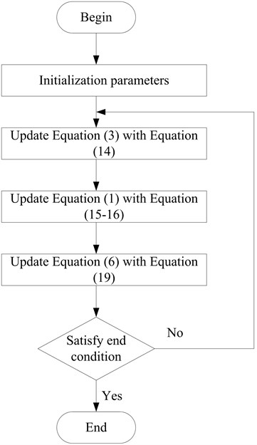
3.4. Algorithm flow

The IGOA algorithm flow is shown in Fig. 1.

4. IGOA-LSSVM based device fault identification steps

The improved GOA and LSSVM for state prediction of power mechanical equipment is to build a nonlinear model between the input and output quantities, which core is to determine two important parameters $c$ and $σ$ in the LSSVM, which have a very significant impact on the predictive capability of the model.

The specific steps are as follows:

Step 1: Set the dimension in which the Grasshoppers are located in the Grasshopper optimization algorithm, the entire number of Grasshopper population, the initial values of the relevant algorithm parameters, and the maximum number of algorithm iterations to run. To set the relevant parameters of the LSSVM neural network, it is required to form a set of parameters $c$ and $σ$ in the LSSVM, and compare the set of parameters with the Grasshopper individuals one by one, so that the best set of parameters can be obtained by involving the optimal Grasshopper individuals, that is, the optimal parameters of the LSSVM.

Step 2: Optimize each of the three improved strategies in GOA according to the improved three-ratio method.

Step 3: In the Grasshopper algorithm individual fitness function, the middle decision function is used in LSSVM, and in the iteration process, the individual fitness value of the Grasshopper is compared with the current individual optimal fitness value, and if the former fitness value is better than the latter, the latter is directly replaced; otherwise, it remains unchanged.

Step 4: When the algorithm reaches the maximum number of iterations, the algorithm ends, so the optimal Grasshopper individuals correspond to the optimal $c$ and $σ$ .

Fig. 1Flow chart of the algorithm in this paper

5. Simulation

5.1. Algorithm performance

In this paper, the IGOA algorithm and the GOA algorithm are compared under six benchmark test functions (Table 1) in different dimensions (2-dimensional, 5-dimensional and 30-dimensional). Moreover, respective parameters and set for 100 iterations are selected for these algorithms, and the simulation results are obtained with the help of Matlab2012 simulation platform as shown in Table 2.

Table 1Benchmark function

Function No	Benchmark function
F1	$\sum_{1}^{n} x^{2}$
F2	$\sum_{i = 1}^{n} (\sum_{j = 1}^{i} x_{j})$
F3	$\sum_{i = 1}^{n - 1} [100 (x_{i + 1} - x_{i}^{2})^{2} + (x_{i} - 1)^{2}]$
F4	$20 e x p (- \frac{1}{5} \sqrt{\frac{1}{n} \sum_{i = 1}^{n} x_{i}^{2}}) - e x p (\frac{1}{n} \sum_{i = 1}^{n} \cos (2 π x_{i}))$
F5	$\sum_{i = 1}^{n} (x_{i}^{2} - 10 c o s (2 π x_{i}) + 10)$
F6	$m a x (a b s (x_{i}))$

Table 2 shows the comparison of the optimal values and variances of the two algorithms in different dimensions of six benchmark functions, and it is found that the difference between the optimal values and variances of the two algorithms in 2 dimensions is not large. The difference between the two algorithms gradually increases as the dimensionality increases, and when the dimensionality reaches 30 dimensions, the optimal value and variance of the two algorithms gradually increase, and the difference between the two algorithms is larger when it is in the F1 and F3 functions. From Table 2, it can be found that IGOA has better performance compared with the GOA algorithm, which also evidences that the improved IGOA can significantly improve the performance of the algorithm, especially in the higher dimensionality. Fig. 2. shows the comparison of the fitness values of the two algorithms. From the figure, it is found that the curves of both algorithms show a decreasing trend as the number of iterations gradually increases, but the IGOA algorithm obtains the optimal value when the number of iterations is 80, which indicates that the performance of the improved algorithm is significantly improved.

Fig. 2Comparison of adaptation values of two algorithms

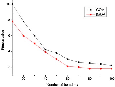
Table 2Optimization results of two algorithms in different benchmark functions

Function	Dimension	Algorithm	Optimal value	Variance
F1	2	GOA	3.172	1.614
	2	IGOA	1.324	0.288
	5	GOA	1.427e-9	1.831e-8
	5	IGOA	2.174e-12	3.932e-11
	30	GOA	3.724e-11	5.212e-11
	30	IGOA	2.294e-14	6.193e-13
F2	2	GOA	3.412	3.532
	2	IGOA	2.814	2.843
	5	GOA	1.437e-10	3.414e-8
	5	IGOA	1.272e-14	4.243e-10
	30	GOA	3.143e-14	3.832e-11
	30	IGOA	1.415e-16	6.941e-13
F3	2	GOA	3.913	1.824
	2	IGOA	2.982	1.392
	5	GOA	3.397e-11	3.281e-9
	5	IGOA	2.912e-13	4.812e-11
	30	GOA	3.628e-12	3.512e-13
	30	IGOA	4.295e-17	7.713e-14
F4	2	GOA	4.812e-4	3.184e-3
	2	IGOA	7.823e-5	1.628e-4
	5	GOA	1.915e-10	3.274e-7
	5	IGOA	2.112e-13	4.132e-11
	30	GOA	7.276e-17	5.131e-12
	30	IGOA	1.832e-17	9.334e-14
F5	2	GOA	1.671e-3	2.134e-2
	2	IGOA	1.015e-4	1.717e-2
	5	GOA	1.856e-11	1.901e-8
	5	IGOA	2.212e-16	6.012e-11
	30	GOA	9.274e-15	4.182e-13
	30	IGOA	2.431e-17	7.342e-15
F6	2	GOA	2.312e-3	1.824e-2
	2	IGOA	3.914e-4	4.124e-3
	5	GOA	3.216e-12	2.815e-10
	5	IGOA	1.312e-13	5.712e-10
	30	GOA	9.178e-13	9.212e-11
	30	IGOA	2.373e-14	8.272e-10

5.2. Fault diagnosis

The internal faults of transformers can be mainly classified into electrical and thermal faults according to their fault phenomena. Therefore, the fault causes are generally divided into high temperature overheating, medium and low temperature overheating, high-energy discharge, low-energy discharge and partial discharge. When a fault occurs in a transformer, hydrogen, methane, ethylene, acetylene and other gases dissolve in the insulating oil of the transformer, and the specific type of fault in the transformer is determined based on the content of these gases in the oil. Therefore, data collection and sample classification are carried out in this paper.

5.2.1. Sample collection

Since the operating condition of a transformer is directly related to the content of dissolved gases in the oil, representative data samples are selected here for model creation. Due to the great variability and dispersion between the volumes of various gas components, the input data for training are first pre-processed here in order to reduce the impact caused by the order-of-magnitude differences between them and to speed up the training. In this paper, the training and test sets are processed by normalization, and the specific formulas are shown below:

24

\bar{X} = \frac{x_{i} - x_{m i n}}{x_{m a x} - x_{m i n}},

where, $x_{i}$ denotes the original raw gas data, $x_{m a x}$ and $x_{m i n}$ denote the maximum and minimum values of the raw gas data, respectively, and $\bar{X}$ denotes the normalized gas data.

5.2.2. Sample classification

According to the improved three-ratio method of gas characteristics, this paper divides the transformer operating status into 6 categories, namely, high-energy discharge, low-energy discharge, high temperature overheating, medium and low temperature overheating, partial discharge, and normal state. In addition, it introduces the corresponding coding system, which is shown in Table 3. Through the model in this paper, the optimized penalty factor $c$ and the kernel height basis function parameter group $σ$ are used to train the model using the training samples in the original DGA [17] data, and the test samples are used to test and evaluate the model.

Table 3Sample classification

No	Category
1	High-energy discharge
2	Low-energy discharge
3	High temperature overheating
4	Medium to low temperature overheating
5	Partial discharge
6	Normal state

5.2.3. Example analysis

In order to verify finally that the transformer’s mechanical fault diagnosis model based on the improved algorithm optimized support vector machine proposed in this paper is equally effective when more data are available. Here in this paper, 260 sets of DGA data collected are classified according to the procedure from Table 4. Among the 260 sets of sample data collected, they are divided into six categories, of which 170 sets of sample data are available in the training set, and the remaining 90 sets are used as the test set sample data. Among them, 1-45 belong to the first category (high-energy discharge), 46-90 belong to the second category (low-energy discharge), 91-135 belong to the third category (high-temperature overheating), 136-180 belong to the fourth category (medium-low temperature overheating), 181-225 belong to the fifth category (partial discharge), and 226-260 belong to the sixth category (normal state). And in the first five operating states of the original DGA data grouped into 30 groups as the training set, the other 1-55 groups as the test set; from the sixth operating state of the data grouped into 20 groups as the training set, and the remaining 1-5 groups were put into the test set. The specific training set and test set sample labels are shown in Table 4.

Table 4Training set and test set samples

Sample tags	1	2	3	4	5	6
Test sets	30	30	30	30	30	20
Sample set	15	15	15	15	15	15

The test failure results are shown in Table 5. The table demonstrates that the algorithm in this paper has good results in six fault cases, with the average detection rate above 93 %. Thus, the IGOA-LSSVM proposed in this paper has good results in the detection process, although the recognition accuracy in high temperature overheating is lower than 90 %, i.e. the gas characteristics of this fault are not obvious enough and are easily influenced by the rest of the fault characteristics.

Table 5Failure test results

Fault type	Number of tests	Number of correct judgments	Accuracy rate
High-energy discharge	15	14	93.3 %
Low-energy discharge	15	14	93.3 %
High temperature overheating	15	13	86.7 %
Medium to low temperature overheating	15	15	100 %
Partial discharge	15	14	93.3 %
Normal state	15	14	93.3 %

5.2.4. Comparison of diagnosis effect

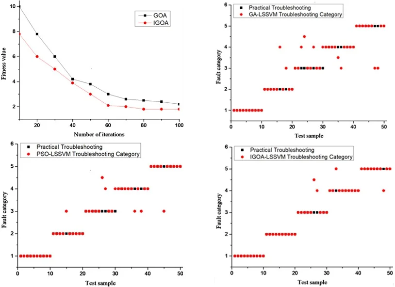
In order to illustrate further the effectiveness of the algorithm in diagnostic prediction, this paper selected the least squares vector machine based on the Ant colony algorithm and the least squares vector machine based on the Particle swarm algorithm for comparison with the algorithm applied in this paper. The authors randomly selected 50 test samples for each experiment. The experimental results are shown in Fig. 3.-Fig. 5.

Fig. 3GA-SVM fault diagnosis classification results

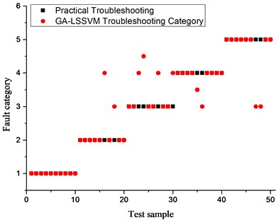
Fig. 4PSO-SVM fault diagnosis classification results

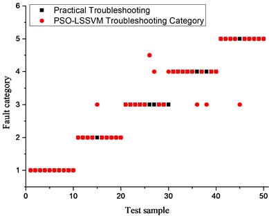
Fig. 5IGOA-SVM fault diagnosis classification results

As shown in Fig. 3, when a GA-LSSVM model is used for transformer fault diagnosis, no faults appear for the high energy discharge diagnosis: 3 faults for low-energy discharge diagnosis; 3 faults for high-temperature overheating diagnosis; 2 faults for medium- and low-temperature overheating diagnosis; 2 faults for partial discharge diagnosis, and the comprehensive fault diagnosis rate is 82 %. As can be derived from Fig. 4, when the PSO-LSSVM model is used for transformer fault diagnosis, no fault appears in the high-energy discharge diagnosis, only one low energy discharge diagnosis error but no fault. Two high temperature overheating diagnosis errors also appear without a fault. Two medium and low temperature overheating diagnoses revealed no fault, only one partial discharge diagnosis error without fault. So the comprehensive fault diagnosis rate is 88 %. As can be derived from Fig. 5, when the IABC-LSSVM model is applied for a transformer fault diagnosis, the high-energy discharge diagnosis and the low-energy discharge diagnosis reveal no fault. One high-temperature overheating diagnosis error appears without fault. Only two medium and low-temperature overheating diagnoses and one partial discharge diagnosis revealed errors without fault. The comprehensive fault diagnosis rate is 92 %. Therefore, from the results in Fig. 3-Fig. 5, the IGOA-LSSVM proposed in this paper has a good effect for diagnosing faults.

6. Conclusions

To improve the ability to identify mechanical faults in power transformers, the authors propose an IGOA-LSSVM fault diagnosis model based on the IGOA. To improve the prediction of LSSVM, they created an IGOA model based on GOA algorithm using three strategies: self-learning factor, proportional weight coefficient and Levy flight, and used it to optimize the LSSVM parameters. In the simulation experiments, the IGOA-LSSVM has better recognition effect compared with ACO-LSSM and PSO-LSSVM models for the identification of five power transformer faults. In the next step, the authors are going to improve further the fault diagnosis method.

References

Y.-J. Sun, S. Zhang, C.-X. Miao, and J.-M. Li, “Improved BP neural network for transformer fault diagnosis,” (in Chinese), Journal of China University of Mining and Technology, Vol. 17, No. 1, pp. 138–142, Mar. 2007, https://doi.org/10.1016/s1006-1266(07)60029-7

Publisher
X. Yang, W. Chen, A. Li, C. Yang, Z. Xie, and H. Dong, “BA-PNN-based methods for power transformer fault diagnosis,” Advanced Engineering Informatics, Vol. 39, pp. 178–185, Jan. 2019, https://doi.org/10.1016/j.aei.2019.01.001

Publisher
S.-W. Fei and X.-B. Zhang, “Fault diagnosis of power transformer based on support vector machine with genetic algorithm,” Expert Systems with Applications, Vol. 36, No. 8, pp. 11352–11357, Oct. 2009, https://doi.org/10.1016/j.eswa.2009.03.022

Publisher
T. Kari et al., “Hybrid feature selection approach for power transformer fault diagnosis based on support vector machine and genetic algorithm,” IET Generation, Transmission and Distribution, Vol. 12, No. 21, pp. 5672–5680, Nov. 2018, https://doi.org/10.1049/iet-gtd.2018.5482

Publisher
S. F. Cheng, X. H. Cheng, and L. Yang, “Application of wavelet neural network with improved particle swarm optimization algorithm in power transformer fault diagnosis,” (in Chinese), Power system Protection and Control, Vol. 42, No. 19, pp. 37–42, 2014, https://doi.org/10.7667/j.issn.1674-3415.2014.19.006

Publisher
B. Zeng, J. Guo, W. Zhu, Z. Xiao, F. Yuan, and S. Huang, “A transformer fault diagnosis model based on hybrid grey wolf optimizer and LS-SVM,” Energies, Vol. 12, No. 21, p. 4170, Nov. 2019, https://doi.org/10.3390/en12214170

Publisher
R. Naresh, V. Sharma, and M. Vashisth, “An integrated neural fuzzy approach for fault diagnosis of transformers,” IEEE Transactions on Power Delivery, Vol. 23, No. 4, pp. 2017–2024, Oct. 2008, https://doi.org/10.1109/tpwrd.2008.2002652

Publisher
L. Dong, D. Xiao, Y. Liang, and Y. Liu, “Rough set and fuzzy wavelet neural network integrated with least square weighted fusion algorithm based fault diagnosis research for power transformers,” Electric Power Systems Research, Vol. 78, No. 1, pp. 129–136, Jan. 2008, https://doi.org/10.1016/j.epsr.2006.12.013

Publisher
P. Purkait and S. Chakravorti, “Time and frequency domain analyses based expert system for impulse fault diagnosis in transformers,” IEEE Transactions on Dielectrics and Electrical Insulation, Vol. 9, No. 3, pp. 433–445, Jun. 2002, https://doi.org/10.1109/tdei.2002.1007708

Publisher
D. Ma, Y. Liang, X. Zhao, R. Guan, and X. Shi, “Multi-BP expert system for fault diagnosis of power system,” Engineering Applications of Artificial Intelligence, Vol. 26, No. 3, pp. 937–944, Mar. 2013, https://doi.org/10.1016/j.engappai.2012.03.017

Publisher
M. Demetgul, K. Yildiz, S. Taskin, I. N. Tansel, and O. Yazicioglu, “Fault diagnosis on material handling system using feature selection and data mining techniques,” Measurement, Vol. 55, pp. 15–24, Sep. 2014, https://doi.org/10.1016/j.measurement.2014.04.037

Publisher
Y. Miao et al., “A review on the application of blind deconvolution in machinery fault diagnosis,” Mechanical Systems and Signal Processing, Vol. 163, p. 108202, Jan. 2022, https://doi.org/10.1016/j.ymssp.2021.108202

Publisher
W. Deng, Z. Li, X. Li, H. Chen, and H. Zhao, “Compound fault diagnosis using optimized MCKD and sparse representation for rolling bearings,” IEEE Transactions on Instrumentation and Measurement, Vol. 71, pp. 1–9, 2022, https://doi.org/10.1109/tim.2022.3159005

Publisher
Q. Song and P. Jiang, “A multi-scale convolutional neural network based fault diagnosis model for complex chemical processes,” Process Safety and Environmental Protection, Vol. 159, pp. 575–584, Mar. 2022, https://doi.org/10.1016/j.psep.2021.11.020

Publisher
S. Saremi, S. Mirjalili, and A. Lewis, “Grasshopper optimisation algorithm: theory and application,” Advances in Engineering Software, Vol. 105, pp. 30–47, Mar. 2017, https://doi.org/10.1016/j.advengsoft.2017.01.004

Publisher
A. M. Edwards et al., “Revisiting Lévy flight search patterns of wandering albatrosses, bumblebees and deer,” Nature, Vol. 449, No. 7165, pp. 1044–1048, Oct. 2007, https://doi.org/10.1038/nature06199

Publisher
X. F. Tian, “Research on transformer fault diagnosis based on improved bat algorithm optimized support vector machine,” (in Chinese), Heilongjiang Electric Power, Vol. 41, No. 1, pp. 11–15, 2019, https://doi.org/10.13625/j.cnki.hljep.2019.01.003

Publisher

Cited by

Research on transformer fault diagnosis method based on ACGAN and CGWO-LSSVM

Shan Guan | Tong-yu Wu | Hai-qi Yang

(2024)

Research on the flow characteristics identification of steam turbine valve based on FCM-LSSVM

(2023)

Multidimensional analysis of engineering cost database based on descriptive data mining

Dandan Ke | Jingyi Dai

(2023)

About this article

Received

07 February 2022

Accepted

10 May 2022

Published

08 June 2022

SUBJECTS

Fault diagnosis based on vibration signal analysis

DOI

https://doi.org/10.21595/jve.2022.22439

Keywords

power transformer

fault prediction

grasshopper optimization algorithm

This is an open access article distributed under the Creative Commons Attribution License, which permits unrestricted use, distribution, and reproduction in any medium, provided the original work is properly cited.

Previous article in issue Previous Next article in issue Next

Research article

2024 02 21

Research on automatic detection of gradual fault of high voltage electric energy metering transformer based on fuzzy rough set and whale optimization algorithm

Chunguang Wang, Zhiwu Wu, Tianfu Huang, Xiang Wu, Hanbin Huang

Research article

2017 12 31

A novel intelligent fault diagnosis method of rotating machinery based on deep learning and PSO-SVM

Peiming Shi, Kai Liang, Dongying Han, Ying Zhang

Research article

2017 08 15

Fault detection and diagnosis of rotating machinery using modified particle filter

Ke Li, Yiya Liu, Jingjing Wu, Lei Su, Peng Chen

Research article

2017 06 30

Adaptive machinery fault diagnosis based on improved shift-invariant sparse coding

Limin Li

Y. Chen, “Research on IGOA-LSSVM based fault diagnosis of power transformers,” Journal of Vibroengineering, Vol. 24, No. 7, pp. 1262–1274, Jun. 2022, https://doi.org/10.21595/jve.2022.22439

Copy Extrica

Copied to clipboard!

TY  - JOUR
DO  - 10.21595/jve.2022.22439
UR  - https://doi.org/10.21595/jve.2022.22439
TI  - Research on IGOA-LSSVM based fault diagnosis of power transformers
T2  - Journal of Vibroengineering
AU  - Chen, Yunsheng
PY  - 2022
DA  - 2022/06/08
PB  - JVE International Ltd.
SP  - 1262-1274
VL  - 24
IS  - 7
SN  - 1392-8716
SN  - 2538-8460
ER  - 

Copy Ris

Copied to clipboard!

@article{Chen_2022,
	doi = {10.21595/jve.2022.22439},
	url = {https://doi.org/10.21595/jve.2022.22439},
	year = 2022,
	month = {jun},
	publisher = {{JVE} International Ltd.},
	volume = {24},
	number = {7},
	pages = {1262--1274},
	author = {Yunsheng Chen},
	title = {Research on {IGOA}-{LSSVM} based fault diagnosis of power transformers},
	journal = {Journal of Vibroengineering}
}

Copy Bibtex

Copied to clipboard!

[1]Y. Chen, “Research on IGOA-LSSVM based fault diagnosis of power transformers,” Journal of Vibroengineering, vol. 24, no. 7, pp. 1262–1274, Jun. 2022, doi: 10.21595/jve.2022.22439.

Copy IEEE

Copied to clipboard!

Chen, Yunsheng. “Research on IGOA-LSSVM Based Fault Diagnosis of Power Transformers.” Journal of Vibroengineering 24, no. 7 (June 8, 2022): 1262–74. https://doi.org/10.21595/jve.2022.22439.

Copy Chicago

Copied to clipboard!

Research on IGOA-LSSVM based fault diagnosis of power transformers

Abstract

1. Introduction

2. Basic algorithm description

2.1. Grasshopper optimization algorithm

2.2. LSSVM

3. IGOA

3.1. Self-learning factor

3.2. Proportional weight coefficient optimization

3.3. Levy flight optimization and individual optimization search

3.4. Algorithm flow

4. IGOA-LSSVM based device fault identification steps

5. Simulation

5.1. Algorithm performance

5.2. Fault diagnosis

5.2.1. Sample collection

5.2.2. Sample classification

5.2.3. Example analysis

5.2.4. Comparison of diagnosis effect

6. Conclusions

References

Cited by

About this article

Related Articles