A gear fault diagnosis method based on variational mode decomposition and multi-scale discrete entropy

Zhang, Tao; Chen, Yongqi; Chen, Yang; Shen, Qian; Dai, Qinge

doi:10.21595/jve.2023.23515

Journal of Vibroengineering

Browse Journal

Submit article

Published: 21 January 2024

Check for updates

A gear fault diagnosis method based on variational mode decomposition and multi-scale discrete entropy

Tao Zhang¹

Yongqi Chen²

Yang Chen³

Qian Shen⁴

Qinge Dai⁵

^{1, 2, 3, 5}College of Science and Technology, Ningbo University, Ningbo, 315211, P. R. China

⁴Ningbo Xin Yue Electronic Technology Co., Ltd., Ningbo, 315211, P. R. China

Corresponding Author:

Qian Shen

Cite the article Download PDF

Downloads 82

Abstract

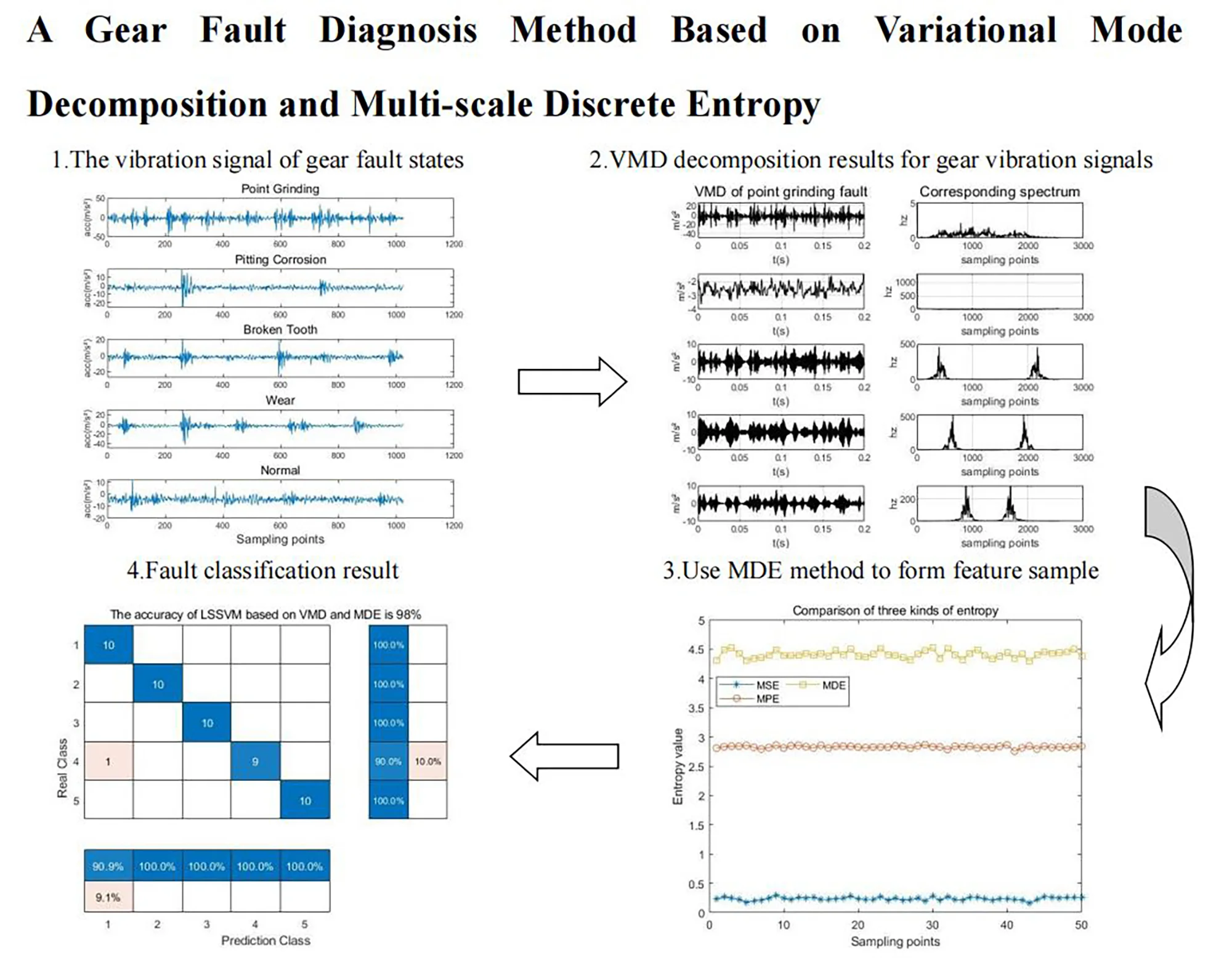
Aiming at monitoring of gearbox faults, a gear fault feature extraction method based on variational mode decomposition (VMD) and multi-scale discrete entropy (MDE) is proposed in this paper. Firstly, the gear fault signal is decomposed into a series of intrinsic modal function (IMF) by VMD with selected parameters; Secondly, the decomposed IMF are extracted by MDE feature extraction method to form a feature sample set; Finally, the least square support vector machine (LSSVM) is used to classify the data set after feature extraction. The experiment results show that the proposed method owns the higher fault diagnosis accuracy than the traditional multi-scale entropy methods.

A gear fault diagnosis method based on variational mode decomposition and multi-scale discrete entropy

Highlights

VMD is proposed to decompose gear fault characteristics.
MDE is proposed to extract gear fault features.
VMD, MDE and LSSVM are applied into gear fault diagnosis system can distinguish different gear fault types with a higher accuracy than traditional methods.

1. Introduction

The occurrence of mechanical faults in the gearbox can seriously affect the normal operation, even causing economic losses [1]. Therefore, it is necessary to monitor and analyze the gears in operation, which is of great significance for the later maintenance of the equipment. In the case of gear wear, broken teeth, pitting corrosion, point grinding and so on, the fault signal shows the characteristics of non-linearity, non-stationary [2]. The commonly used methods in the field of fault diagnosis include time domain analysis, frequency domain analysis, and time-frequency domain analysis. Zhang et al. [3] improved the accuracy of the final evaluation of bearing degradation performance by extracting multiple time domain and frequency domain features of bearing vibration signals and forming high-dimensional and multi-domain feature vectors. For non-linearity and non-stationary fault signal, the traditional time domain analysis such as skewness, kurtosis, variance and other indicators and frequency domain analysis can't well show its fault characteristics. At this time, the time-frequency domain decomposition method should be considered [4]. Empirical mode decomposition (EMD) [5] is suitable for dealing with non-stationary and nonlinear signals, but the intrinsic mode function (IMF) decomposed by EMD is prone to end-point effects and modes. In order to solve the above problems, Wu et al. [6] proposed the ensemble empirical mode decomposition (EEMD) by taking advantage the Gaussian white noise which has a uniform frequency distribution. However, the white noise in the signal after the residual EEMD decomposition will lead to the reconstruction error of the signal [7]. In order to solve the above problems, Dragomiretskiyet al. [8] proposed a new non-recursive and adaptive signal processing method variational mode decomposition in 2014. By constructing and solving constrained variational problems, this method can effectively alleviate the modal aliasing and boundary effects in conventional decomposition methods [9]. Moreover, VMD can effectively handle the background noise, which is suitable for the analysis of non-stationary and non-linear vibration signals [10]. Li et al. [11] used the combination of VMD and minimum entropy deconvolution method for bearing faults that occurred in the background of strong noise. Li et al. [12] selected the IMF obtained by VMD that has a good correlation with the original signal as the feature component, and its validity was experimentally demonstrated.

When there is a partial failure of the gear, periodic shocks will be generated. The information entropy can effectively reflect the information contained in events and is widely used in mechanical fault diagnosis [13]. The commonly used entropy extraction methods are sample entropy, permutation entropy, discrete entropy and so on [14]. However, due to the lack of relevant quantitative indicators, a single entropy to diagnose mechanical faults is not ideal. Therefore, it is necessary to perform multi-scale entropy analysis on the fault signal of the gear. Costa et al. proposed multi-scale sample entropy (MSE) [15]. MSE calculates the mean of adjacent data at different scales of the original signal, obtains a new coarse-grained sequence, and then solves the entropy of the corresponding sequence. Compared with the traditional entropy algorithm, MSE feature extraction has a wider dimension and higher reliability. Jin et al. [16] proposed a bearing fault diagnosis method based on MSE and an improved extreme learning machine. However, sample entropy has certain limitations in determining sample categories. It uses a hard threshold step function, and it is difficult to distinguish categories based on hard thresholds in life. Chen et al. [17] proposed a feature extraction method for ship radiated noise complexity in complex marine environments based on multi-scale permutation entropy (MPE). However, in most cases, multi-scale permutation entropy is not sensitive to signal changes and cannot effectively extract effective information from the signal. Multi-scale discrete entropy (MDE) has the advantages of simple and fast calculation compared to MSE and MPE. MDE is also more sensitive to the data signals such as synchronization frequency, signal amplitude value and signal bandwidth. Zhang [18] used MDE in gear fault diagnosis and experimentally demonstrated the obvious superiority of this method compared with other feature extraction methods.

In recent years, researchers used many methods to recognize the failure types of mechanical parts. Zhao et al. [19] successfully identified the fault type of the bearing by extracting the wavelet packet energy and inputting it into the BP neural network. Yang et al. [20] use a combination of dual-tree complex wavelet transform combined with convolution neural network method to achieve high-precision identification of planetary gear fault types. Support vector machine (SVM) is also a pattern recognition method that can solve problems such as small samples and non-linearity, and it has better learning ability and generalization ability compared with neural networks, so it is widely used in the fault diagnosis of rolling bearings [21, 22]. Least square support vector machine (LSSVM) is an extension of SVM, which solves the problem of too large solution scale in the operation of SVM algorithm, and improves the accuracy and accuracy of nonlinear signal processing. Compared with artificial neural network and other methods, it can overcome the shortcomings of long training time, randomness of training results and over-learning [23,24]. Wang et al. [25] used the combination of discrete wavelet transform and LSSVM for bearing fault diagnosis, and experiments proved that LSSVM classification had good results.

For these advantages, this paper designs a new gear fault diagnosis method based on VMD, MDE and LSSVM. The detail steps of the proposed method are presented as follows: (1) The decomposition layer $k$ of VMD is selected by the maximum criterion of center frequency for the first time, and the gear vibration signal is decomposed by VMD, and IMF components are obtained. (2) MDE method is used to extract the features of each IMF component to form a feature sample set. (3) The acquired feature sample set is divided into training set and test set and input into LSSVM to identify the fault state of the gear.

2. Basic theory

2.1. Principle of VMD

VMD is a new adaptive time-frequency decomposition method. It integrates the concepts of Wiener filtering, Hilbert transform, outlier demodulation, frequency mixing and signal analysis [26]. Through a series of iterations, the original signal can be decomposed into multiple IMF with different center frequencies and bandwidths. The constraint is that the sum of the decomposed modal components is equal to the input signal and the sum of the bandwidths of the decomposed modal components should be minimized, so the constrained model is shown in Eq. (1):

1

\{\begin{array}{l} \underset{{μ_{k}}, {ω_{k}}}{m i n} \{\sum_{k} {‖\partial_{t} [(δ (t) + \frac{j}{π t}) μ_{k} (t)] e^{- j ω_{k} t}‖}_{2}^{2}\}, \\ s . t . \sum_{k} μ_{k} = f, \end{array}

where, $\partial_{t}$ is the partial derivative of $t$ , $δ (t)$ is the impulse function, $μ_{k}$ is the $k$ th modal function, $ω_{k}$ is the center frequency of each mode, and $f$ is the original signal.

On this basis, the quadratic penalty factor $α$ and the lagrange multiplication operator $λ (t)$ are introduced to transform the above variational model into an unconstrained variational model. The transformed Lagrange expression is shown in Eq. (2):

2

L (\{μ_{k}\}, \{ω_{k}\}, λ) = α \sum_{k} {‖\partial_{t} [(δ (t) + \frac{j}{π t}) μ_{k} (t)] e^{- j ω_{k} t}‖}_{2}^{2}

+ {‖f (t) - \sum_{k} μ_{k} (t)‖}_{2}^{2} + ⟨λ (t), f (t) - \sum_{k} μ_{k} (t)⟩,

where, the $α$ parameters are used to ensure the accuracy of the reconstructed signal, which $λ (t)$ can make the constraints more stringent.

The Lagrange expression can be solved using the alternating power multiplier algorithm, and the saddle point of the Lagrange expression can be solved by alternately updating the $μ_{k}^{n + 1}$ , $ω_{k}^{n + 1}$ and $λ^{n + 1}$ . Among them, it can be expressed by Eq. (3):

3

μ_{k}^{n + 1} = \underset{μ_{k} \in X}{a r g m i n} \{α {‖\partial_{t} [(δ (t) + \frac{j}{π t}) μ_{k} (t)] e^{- j ω_{k} t}‖}_{2}^{2} + {‖f (t) - \sum_{i} μ_{i} (t) + \frac{λ (t)}{2}‖}_{2}^{2}\} .

The specific process of the VMD algorithm is as follows:

Step 1: Initialize $μ_{k}^{1}$ , $ω_{k}^{1}$ , $λ_{k}^{1}$ and $n$ .

Step 2: Update $μ_{k}$ :

4

{\overset{\land}{μ}}_{k}^{n + 1} (ω) = \frac{\hat{f} (ω) - \sum_{i \neq k} {\hat{μ}}_{i} (ω) + \frac{\hat{λ} (ω)}{2}}{1 + 2 α (ω - ω_{k})^{2}} .

Step 3: Update:

5

ω_{k} ω_{k}^{n + 1} = \frac{\int_{0}^{\infty} ω {|{\hat{μ}}_{k} (ω)|}^{2} d ω}{\int_{0}^{\infty} {|{\hat{μ}}_{k} (ω)|}^{2} d ω} .

Step 4: Update $λ$ :

6

{\hat{λ}}^{n + 1} (ω) \leftarrow {\hat{λ}}^{n} (ω) + τ [\hat{f} (ω) - \sum_{k} {\hat{μ}}_{k}^{n + 1} (ω)] .

Step 5: If:

7

\sum_{k} \frac{{‖{\hat{μ}}_{k}^{n + 1} - {\hat{μ}}_{k}^{n}‖}_{2}^{2}}{{‖{\hat{μ}}_{k}^{n}‖}_{2}^{2}} < ε,

where ( $ε > 0$ , this paper $ε =$ 1×10^-7), then stop the iteration, otherwise return to the second step.

2.2. Multi-scale discrete entropy

Azami et al. proposed a discrete entropy (DE) method [27]. Discrete entropy does not need to rank vector magnitude values in different embedded dimensions like sample entropy. Furthermore, it need not to calculate the distance between two vectors in different embedded dimensions. Therefore, compared with the sample entropy, discrete entropy, DE has more advantages such as faster operation. Moreover, DE effectively solves the influence of the medium amplitude of the embedded vector, and is more sensitive to the changes of synchronization frequency, amplitude value and signal bandwidth.

Since the fault information of the gears in operation is distributed in multiple scales, the fault feature information on other scales will be omitted if only the discrete entropy of a single scale is used for analysis. This paper uses the multi-scale discrete entropy (MDE) method to extract the fault information of gears. The main calculation process is presented as follows:

The multi-scale factor is introduced $τ$ for the time series $U = \{u_{1}, u_{2}, . . . u_{N}\}$ , and the series is divided into multiple non-overlapping sequence segments to obtain a new time series $x_{j}^{τ}$ :

8

x_{j}^{(τ)} = \frac{1}{τ} \sum_{b = (j - 1) τ + 1}^{j τ} u_{b} .

Map sequences $x_{j}^{τ}$ to integer classes with labels ranging from 1 to $c$ . Coarse-grained sequences are mapped to the interval 0 to 1 by introducing a normal cumulative distribution function:

9

y_{j} = \frac{1}{σ \sqrt{2 π}} \int_{}^{x_{j}} e^{\frac{- {(x - r m s)}^{2}}{2 σ^{2}}} d t,

where $r m s$ and $σ$ are the root mean square and standard deviation of the original signal.

Using a linear algorithm to assign $y_{j}$ linearity between 1 to $c$ and introducing the embedding dimension $m$ and delay parameters $d$ , the reconstruction sequence $Z_{i}^{m, c}$ is:

10

Z_{i}^{m, c} = \{Z_{i}^{c}, Z_{i + d}^{c}, . . . Z_{i + (m - 1) d}^{c}\} .

Calculate $c^{m}$ the relative probability of each potential dispersion $π_{v_{0} v_{1} . . . v_{m - 1}}$ mode:

11

p (π_{v_{0} . . . v_{m - 1}}) = \frac{N u m b e r \{i |i \leq N - (m - 1) d, z_{i}^{m, c} h a s t y p e π_{v_{0} . . . v_{m - 1}}\}}{N - (m - 1) d},

Based on the definition of information entropy, the discrete entropy value under a single scale $τ$ is calculated:

12

e (x, m, c, d) = - \sum_{π = 1}^{c^{m}} p (π_{v_{0} . . . v_{m - 1}}) \cdot l n (p (π_{v_{0} . . . v_{m - 1}})) .

Finally, the multi-scale discrete entropy is defined as the set of discrete entropy values at multiple different scales, then the multi-scale discrete entropy is expressed as:

13

M D E = E (x, s, m, c, d) = {[e_{1}, e_{2}, . . . e_{s}]}^{T} .

2.3. Overview of LSSVM

The support vector machine (SVM) needs to reduce the error through the quadratic programming process, and LSSVM transforms the problem into a system of linear equations using the least squares method. It can be seen that LSSVM is based on SVM. It significantly reduces the computation of LSSVM, which can achieve higher classification efficiency. The specific process is as follows.

Let the training data set be $x_{j}$ , $y_{j}$ , where $x_{j}$ is the input of the training data of the dimension $n$ ; $y_{j}$ is the output value of the model. The formula of LSSVM can be expressed as [28]:

14

y (x) = ω^{T} θ + b,

where $θ$ represents the feature map, which converts the complex nonlinear relationship between the output $y$ and the input $x$ in to a linear relationship between $y$ and $θ$ , which $b$ is the bias vector and $ω$ is the weight vector:

15

m i n_{ω, b, e} J (ω, e) = \frac{1}{2} {‖ω‖}^{2} + \frac{1}{2} γ \sum_{i = 1}^{n} {e_{i}}^{2} s . t . y_{i} [ω^{T} ϕ (x_{i}) + b] = 1 - e_{i},

where $γ$ is the regularization parameter, $e_{i}$ is the error term, and $φ (x)$ is the nonlinear mapping function from the original space to the multi-dimensional feature space. The definition of the Lagrange function is:

16

L = \frac{1}{2} {‖ω‖}^{2} + \frac{1}{2} γ \sum_{i = 1}^{N} e_{i}^{2} - \sum_{i = 1}^{N} α_{i} \{y_{i} [ω^{T} ϕ (x_{i}) + b] - 1 + e_{i}\} .

For $ω$ , $b$ , $α_{i}$ and $ε_{i}$ in the above formula find the partial derivative and make it 0, and bring it into the above formula to get the matrix equation:

17

[\begin{array}{l} 0 & - y^{T} \\ y & Ω + γ^{- 1} I \end{array}] [\begin{array}{l} b \\ α \end{array}] = [\begin{matrix} 0 \\ I_{n} \end{matrix}] .

$Ω_{i j} = y_{i} y_{j} ϕ {(x_{i})}^{T} ϕ (x_{j}) = y_{i} y_{j} K (x_{i}, x_{j})$ , $y$ and $I_{n}$ are n-order matrices. Solving the above equations can get a set of $α$ and $b$ , then the LSSVM classification expression can be obtained as:

18

f (x) = s g n [\sum_{i = 1}^{N} α_{i} y_{i} K (x, x_{i}) + b] .

LSSVM solves the original dual problem through the above process. The linear constraints in the optimization goal simplify the solution process and obtains the value of the optimization variables $α$ and $b$ , which is simpler than SVM.

3. The bundling machine gear fault diagnosis experiment

To demonstrate the effectiveness of the method proposed in this paper, experiments are carried out on a motor-drive-gear fault test platform in Fig. 1. The speed of DC motor can reach 1450 rpm. By using a coupling, a shaft is attached to the motor. With the help of the shaft, the motion is transmitted to the gear. The various defect gears are produced in this experiment platform. The accelerometer is connected as the signal detection unit. Fault vibration signals can be stored digitally in a computer through an amplifier and analogue-to-digital converter. The fault vibration signals are then obtained and extracted to different features. The vibration signals are acquired with a sampling rate of 5120 Hz. Five different states of gears are collected: point grinding, pitting corrosion, broken tooth, wear and normal. The sampling length of each fault state is 53248, and their fault signals are shown in Fig. 2.

Fig. 1Motor-drive-gear fault test platform

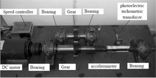
Fig. 2Five kinds of gear fault signals

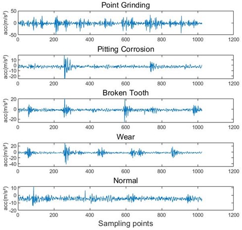
It can be seen that the vibration signal has complex shock characteristics, and it is difficult to identify the fault characteristics. Therefore, VMD is used to decompose the original signal into different IMF components. The vibration signal is divided into 50 groups, and the length of each group is 1024. Taking the normal gear signal as an example, different pre-decomposition modes $k$ are selected for VMD, in which the penalty factor a takes the default value 2000. The main difference of different modes lies in the difference of the central frequency. According to the VMD algorithm, the central frequency of each IMF component obtained from the VMD of the vibration signal will be distributed from low frequency to high frequency. If you want to obtain the optimal preset scale $k$ , the center frequency of the last order IMF component should be the maximum for the first time. Table 1 shows the central frequencies of each IMF component under different modes.

Table 1Center frequency after VMD when taking differentkvalues

Preset scale	Center frequency
Preset scale	IMF1	IMF2	IMF3	IMF4	IMF5	IMF6	IMF7	IMF8
$K =$ 2	25
$K =$ 3	25	545	720
$K =$ 4	25	250	545	940
$K =$ 5	25	250	545	720	940
$K =$ 6	25	250	350	545	720	940
$K =$ 7	25	250	350	545	720	940	1165
$K =$ 8	25	250	350	545	570	720	940	1165

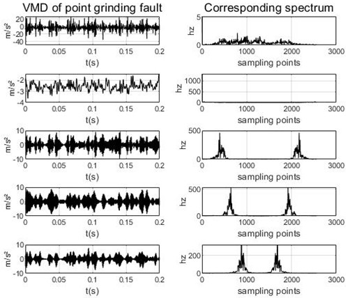
As can be seen from Table 1, the minimum value of the central frequency is taken from the initial preset scale $k = 2$ , and the maximum value of the central frequency tends to be stable when $k = 4$ and $k = 7$ . In order to prevent the mode number $k$ of VMD from being too large and over-decomposing, the $k$ value selected in this paper is 4. The data of a group of gear point grinding faults are decomposed by EMD, EEMD and VMD respectively, in which the sampling frequency of this group of data samples is 5120 Hz, the number of sampling points is 53248, and the signal length of each segment is 1024. The results are shown in Fig. 3, Fig. 4 and Fig. 5.

Fig. 3EMD and its frequency spectrum under gear point grinding

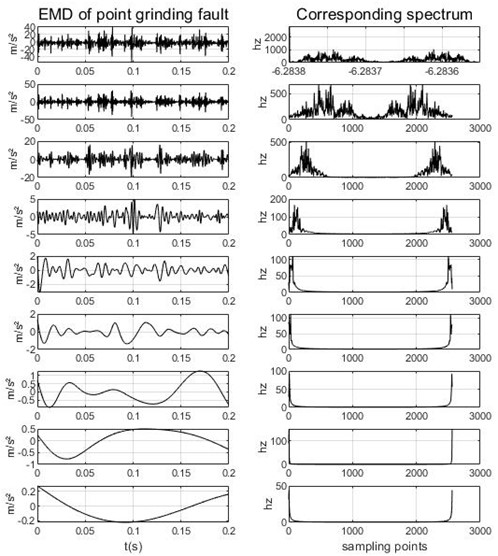
The fact that there are two peaks in each component of the three decomposition graphs is due to the use of bilateral spectra, so there are two peaks symmetrical to each other, which has no effect on the experimental decomposition results. By comparing the intrinsic modal components and their corresponding spectra obtained by the three decomposition methods, we can see that there are many invalid components in EMD and EEMD methods after decomposition, so they cannot extract their corresponding spectrum, and the first component in the EMD map and the first three components in the EEMD map have different degrees of modal aliasing. For VMD, we can see that the IMF components obtained by the decomposition are concentrated near their respective central frequencies, and the frequency domain characteristics are independent of each other, which effectively avoids the problem of modal aliasing, and there are no invalid components. From this, we can know that VMD is better than the other two decomposition methods, which can improve the accuracy of using entropy as fault feature.

Fig. 4EEMD and its frequency spectrum under gear point grinding

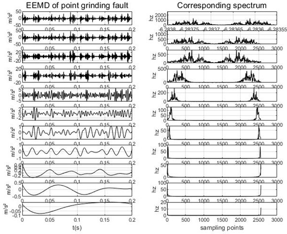
Fig. 5VMD and its frequency spectrum under gear point grinding

For the samples decomposed by the VMD method, their multi-scale sample entropy (MSE), multi-scale permutation entropy (MPE) and multi-scale discrete entropy (MDE) are extracted respectively. Due to the length of each sample segment being 1024, the maximum number of segments for all samples is 50. The length of feature samples extracted by each entropy extraction method is set to 48, forming a 50×48 feature sample dataset. Fig. 6 shows a comparison of the average values of three entropy extraction methods. To demonstrate the correlation between five types of samples extracted by different entropy extraction methods, Pearson correlation coefficient analysis was performed on the samples extracted by different entropy extraction methods, and the results are shown in Fig. 7.

Fig. 6Comparison of three kinds of entropy

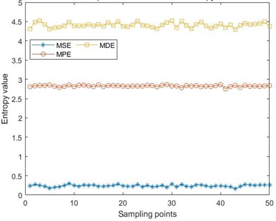
It can be seen from the figure that after taking the average value of the extracted 50×48 feature samples, the samples extracted under the MSE method are stable, but their entropy is between [0, 0.5], which cannot well reflect the characteristics of the original fault signal. The entropy value extracted by MDE method has high stationarity, and the entropy value is also larger than that of the other two extraction methods, indicating that this method can better extract the features of the signal and improve the accuracy of the final fault classification.

Fig. 7Pearson correlation coefficients of three entropy extraction methods

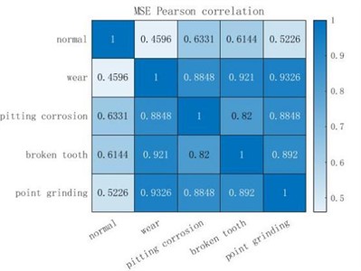
a) MSE Pearson correlation

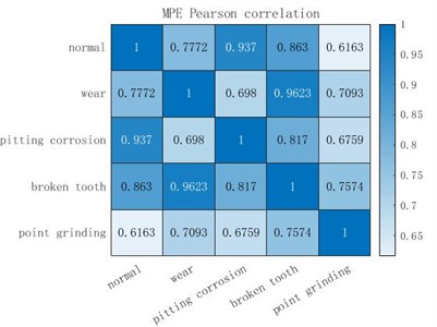
b) MPE Pearson correlation

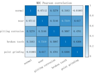
c) MDE Pearson correlation

Pearson correlation coefficient measures the correlation between the two fault types. After taking the absolute value, the larger the correlation coefficient is, the more relevant the two types are. It can be seen from Fig. 7 that the entropy extracted by MSE and MPE has a high correlation coefficient in the two fault states of broken tooth and wear, and the entropy extracted by MSE shows a high correlation between pitting corrosion and wear, point grinding and wear, point grinding and pitting corrosion, point grinding and broken teeth, which is not conducive to the final fault diagnosis and classification. Similarly, MPE also shows a high correlation between broken teeth and normal, pitting corrosion and normal fault data. However, for the data extracted by MDE, all fault samples show a lower correlation than the other two methods, and even the correlation between normal and point grinding, normal and wear data is very low, which is very conducive to the final fault diagnosis classification. To sum up, the entropy extracted by MDE has a better non-correlation between each fault type than the other two methods, which can make the final fault diagnosis more accurate.

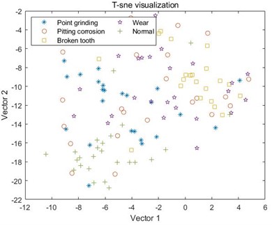
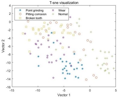
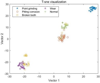
All the extracted data feature samples are visually analyzed by T-sne, and the results are shown in Fig. 8.

By observing A, B, and C in the graph, it can be seen that the data samples have been decomposed using three different decomposition methods, and the samples extracted using the MSE entropy extraction method exhibit different correlations. There is a serious mixing phenomenon between the sample points in A and B, and it is impossible to observe any obvious boundaries between different types of samples through visualization.

Fig. 8Visual analysis results of T-sne

a) MSE combined with EMD

b) MSE combined with EEMD

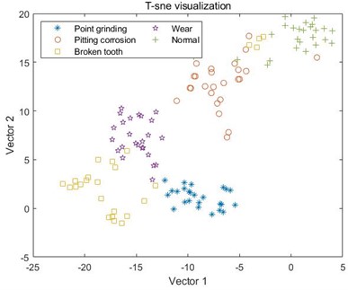
c) MSE combined with VMD

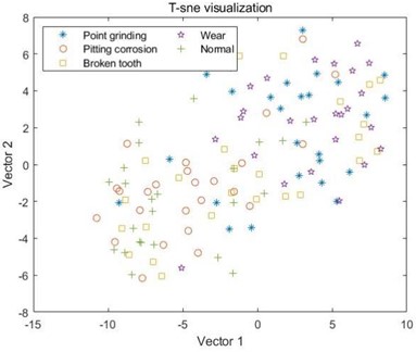
d) MPE combined with EMD

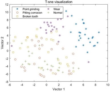
e) MPE combined with EEMD

f) MPE combined with VMD

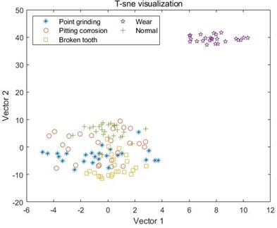
g) MDE combined with EMD

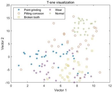
h) MDE combined with EEMD

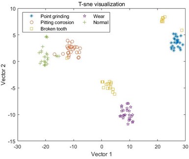
i) MDE combined with VMD

For the samples decomposed by VMD, as shown in C, it can be seen that the five samples have started to differentiate, but it is not particularly obvious, and there is still varying degrees of mixing between the samples. Like MSE, the samples extracted by MPE also have the same problem, where different types of samples in D and E cannot be distinguished at all, and the sample points are mixed together; However, the samples decomposed by VMD have achieved a certain degree of differentiation, and the samples under point grinding fault have been distinguished from the other four fault samples. However, there is still a mixing phenomenon between the other four samples, as shown in F. In G and H, the differentiation between samples is still not very clear, and only wear fault samples can be distinguished in G. This indicates that EMD and EEMD methods cannot process the data well, resulting in poor differentiation between extracted feature samples. Finally, from I, it can be seen that after the VMD method decomposition, only a small portion of the feature data extracted by MDE under broken tooth fault is separated into two parts, and the remaining data samples are mapped to their respective regions, with a good degree of differentiation. The results indicate that the data extracted by combining MDE and VMD methods can effectively distinguish different types of fault samples, ultimately achieving high-precision fault classification.

After obtaining the feature sample set, LSSVM classifier is used to perform fault classification on the entropy samples extracted by the MDE method. The first 40 groups of 50 sample data are used as the training set, and the remaining 10 groups of data are used as the test set. For the regularization parameters and kernel parameters of LSSVM, particle swarm optimization algorithm is used to iterate them. The range of regularization parameters and kernel parameters is set to [0.1, 200], the minimum and maximum speed is [–10, 10], and the particles used for optimization are 10. Each iteration is carried out 10 times, and the maximum accuracy is taken as the objective function. The optimal parameter combination is selected to be substituted into the LSSVM classifier for fault classification of the training and testing sets. Moreover, to verify the superiority of the proposed MDE based on VMD method, MSE and MPE are also used to extract the rolling bearing fault feature vectors at the same time and input them into LSSVM for pattern recognition. In order to avoid overfitting, LSSVM uses cross validation during training to separate the training and testing samples, improving its generalization ability. The specific approach is to divide the samples into 5 sub sets, with one individual sub sample retained as the validation model data, and the other 4 samples used for training. Cross validation is repeated 5 times, with each sub sample validated once, and an average of 5 times ultimately leads to a single estimate. This method repeatedly uses randomly generated sub samples for training and validation, with each result validated once, effectively avoiding the occurrence of over learning and under learning states. The random experiment was repeated 30 times and the final results were averaged. The comparison experiment results are presented in Fig. 9 and Table 2.

For the decomposition method VMD, the average accuracy of MDE is 98 %, while the average accuracy of MPE is 90 %, and the average accuracy of MSE is 92%. The main reason is that MDE is more sensitive to the data signals such as synchronization frequency, signal amplitude value and signal bandwidth. Furthermore, one can compare the accuracy of three decomposition method. For VMD, the average accuracy of MDE, MPE and MSE is 98 %, 90 % and 92 % respectively. For EEMD, the average accuracy of MDE, MPE and MSE is 86 %, 78 % and 78 %. For EMD, the average accuracy of MDE, MPE and MSE is 84 %, 62 % and 66 %. VMD obtain the highest accuracy. The main reason is that VMD integrates the Wiener filter, which can effectively alleviate the modal aliasing and boundary effects of EMD and EEMD. In a word, for the same decomposition method, it can be seen that the data samples extracted by MDE can obtain better accuracy than the other two methods. For the same entropy extraction method, the signal decomposed by VMD can be get better classification accuracy.

In order to further demonstrate the superiority of LSSVM classifier, nine samples were input into SVM classifier again for fault diagnosis. The random experiment was repeated 30 times and the average value was taken. From Table 2, we can see that the use of SVM classifiers has resulted in a small reduction in runtime, both of which remain around 0.9 seconds. For the signals decomposed by EMD method, the classification accuracy of the extracted MDE entropy and the accuracy of MSE and MPE methods are not significantly different, with 59 %, 58 %, and 60 % respectively; For the signal decomposed by the EEMD method, the MDE entropy accuracy is higher than the other two methods, reaching 79 %; For the signals decomposed by the VMD method, the MDE method has greatly improved the final accuracy, far surpassing the other two entropy extraction methods, reaching 96 %, once again proving the effectiveness of the VMD and MDE methods mentioned earlier. In terms of accuracy of different classifiers, the final accuracy of using SVM classifier is lower than that of using LSSVM classifier. For the VMD-MDE method proposed in this article, the accuracy of SVM is also 2 % lower than that of LSSVM. In summary, although LSSVM is slightly longer in runtime than SVM classifier, its classification accuracy is higher than SVM classifier, which also demonstrates the superiority of LSSVM classifier.

Table 2Diagnostic accuracy rates under different methods

Decomposition method	Extraction method	LSSVM Accuracy	Operation time	SVM Accuracy	Operation time
EMD	MSE MPE MDE	66 % 62 % 84 %	1.62931 s 1.54487 s 1.51179 s	58 % 60 % 59 %	0.8291 s 0.8533 s 0.8091 s
EEMD	MSE MPE MDE	78 % 78 % 86 %	1.56038 s 1.54516 s 1.73575 s	70 % 75 % 79 %	0.8601 s 0.8619 s 0.9210 s
VMD	MSE MPE MDE	92 % 90 % 98 %	1.71418 s 1.67633 s 1.51163 s	90 % 86 % 96 %	0.9179 s 0.8585 s 0.8494 s

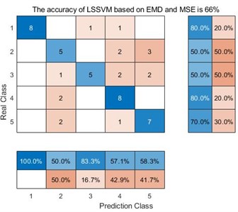
In the confusion matrix classification diagram, label 1 is the normal state signal, label 2 is the wear state signal, label 3 is the pitting corrosion state signal, label 4 is the broken tooth state signal, and label 5 is the point grinding state signal. From Fig. 9, it can be seen that in all 9 confusion matrices, the predicted class and the real class are treated as positive and negative examples in the classifier classification respectively. Therefore, sensitivity is the proportion of accurately classified samples in all predicted classes; And specificity refers to the proportion of correctly classified samples among all real classes. Taking the average of the proportion of correctly classified samples between the predicted class and the real class yields Table 3.

Fig. 9Classification results of 9 different methods

a) LSSVM based on EMD and MSE

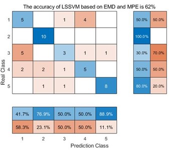
b) LSSVM based on EMD and MPE

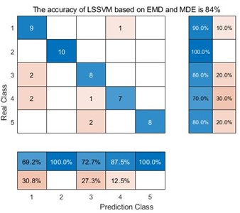
c) LSSVM based on EMD and MDE

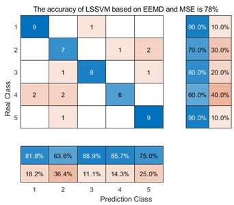
d) LSSVM based on EEMD and MSE

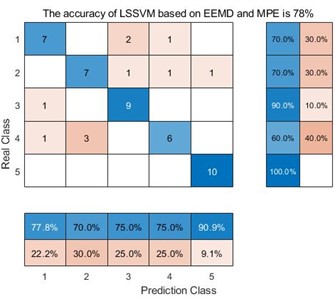
e) LSSVM based on EEMD and MPE

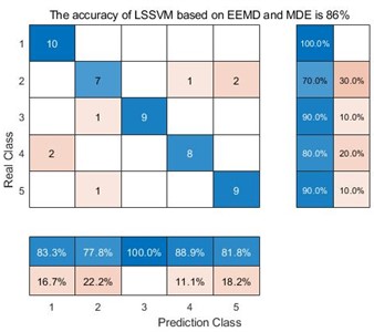
f) LSSVM based on EEMD and MDE

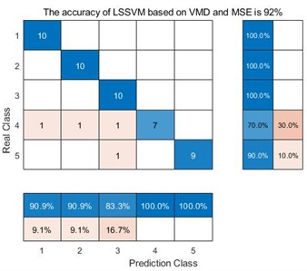
g) LSSVM based on VMD and MSE

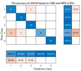
h) LSSVM based on VMD and MPE

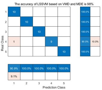
i) LSSVM based on VMD and MDE

From Table 3, we can see that taking the EMD decomposition method as an example, the sensitivity and specificity of the predicted class and the real class are different under different entropy extraction methods. Among them, the MDE method has the highest sensitivity and specificity, indicating that the number of samples misclassified during the diagnostic process is smaller than the other two entropy extraction methods. However, throughout the EEMD and VMD methods, the MDE method has the highest sensitivity and specificity, reaching 86.36 %, 86 % and 98.18 %, 98 % respectively, indicating that the MDE method can effectively avoid misclassifying samples compared to the other two entropy extraction methods. Taking the same entropy extraction method MSE as an example, the sensitivity and specificity of samples decomposed by VMD are much higher than those processed by the other two decomposition methods, reaching 93.02 % and 92 % respectively. This is also true for MPE and MDE methods, where the sensitivity and specificity of samples processed by VMD and extracted by MDE method reach 98.18 % and 98 %, this also proves that the method proposed in this article does have advantages in correctly classifying certain types of samples.

Table 3Sensitivity and specificity of different methods in classifiers

Decomposition method	Extraction method	Sensitivity	Specificity
EMD	MSE MPE MDE	69.74 % 61.5 % 85.88 %	66 % 62 % 84 %
EEMD	MSE MPE MDE	79 % 77.74 % 86.36 %	78 % 78 % 86 %
VMD	MSE MPE MDE	93.02 % 91.36 % 98.18 %	92 % 90 % 98 %

4. Conclusions

In this paper, a gear fault feature extraction method based on VMD and MDE is proposed, and least square support vector machine LSSVM classifier is used to realize fault pattern recognition. First of all, five kinds of data samples of normal, broken teeth, point grinding, wear and pitting corrosion of gears are collected by the gear fault test-bed, and the best decomposition layers are selected by the principle that the center frequency of the decomposed IMF gets the maximum for the first time. The superiority of the VMD method is illustrated by comparing VMD with EMD and EEMD methods. Secondly, MDE method is extracted from the decomposed data, and the samples extracted by multi-scale discrete entropy, multi-scale sample entropy and multi-scale permutation entropy are compared. Pearson correlation coefficient shows the effectiveness of MDE method. Finally, in order to further illustrate the advantages of the proposed method, the samples extracted by EMD-MSE, EEMD-MPE and other methods are visually analyzed by T-sne, and all the data are input into the LSSVM classifier for fault diagnosis and classification. From the comparison results, we can see that the fault diagnosis accuracy obtained by VMD-MDE is 98 %, which is significantly higher than the other eight classification methods. And in the classification of fault samples, the sensitivity and specificity of this method reached 91.18 % and 98 %, indicating that this method can better classify samples correctly. To sum up, the method proposed in this paper has significant advantages.

In the VMD method, the selection of decomposition layers and penalty factor affects the decomposition results, so whether to use the optimization algorithm to find the optimal combination of parameters to make the decomposition results optimal is a problem to be considered.

References

L. Jiang, D. Xiang, P. Mu, and Y. Shen, “Research on robust optimal design of gearbox,” Mechanical Design and Manufacture, pp. 14–16, May 2018, https://doi.org/10.19356/j.cnki.1001-3997.20180626.009

Publisher
L. Yang, Y. Wang, and S. He, “Gear fault diagnosis based on VMD and generalized Warblet transform,” Journal of Mechanical Transmission, Vol. 42, No. 7, pp. 157–161, Jul. 2018, https://doi.org/10.16578/j.issn.1004.2539.2018.07.031

Publisher
L. Zhang, Y. Liu, R. Wu, L. Wang, Z. Chen, and Q. Yan, “Evaluation of bearing performance degradation based on global optimization of an MSET reconstruction model,” Journal of Vibration and Shock, Vol. 42, No. 16, pp. 251–261, Aug. 2023, https://doi.org/10.13465/j.cnki.jvs.2023.16.031

Publisher
S. Chen, “Study on rolling bearing fault diagnosis using improved multiscale sample entropy and parameters optimization SVM,” Master thesis, Jiangsu University, 2020.

Search CrossRef
B. Liu, S. Riemenschneider, and Y. Xu, “Gearbox fault diagnosis using empirical mode decomposition and hilbert spectrum,” Mechanical Systems and Signal Processing, Vol. 20, No. 3, pp. 718–734, Apr. 2006, https://doi.org/10.1016/j.ymssp.2005.02.003

Publisher
Z. Wu and N. E. Huang, “A study of the characteristics of white noise using the empirical mode decomposition method,” Proceedings of the Royal Society of London. Series A: Mathematical, Physical and Engineering Sciences, Vol. 460, No. 2046, pp. 1597–1611, Jun. 2004, https://doi.org/10.1098/rspa.2003.1221

Publisher
B. Yang, J. Zhang, J. Wang, and C. Zhang, “Early fault feature extraction of rolling bearings applying CEEMD-MCKD,” Mechanical Science and Technology for Aerospace Engineering, Vol. 37, No. 12, pp. 1936–1943, May 2018, https://doi.org/10.13433/j.cnki.1003-8728.20180086

Publisher
K. Dragomiretskiy and D. Zosso, “Variational mode decomposition,” IEEE Transactions on Signal Processing, Vol. 62, No. 3, pp. 531–544, Feb. 2014, https://doi.org/10.1109/tsp.2013.2288675

Publisher
X. Zhao, S. Zhang, Z. Li, F. Li, and Y. Hu, “Application of new denoising method based on VMD in fault feature extraction,” Journal of Vibration, Measurement and Diagnosis, Vol. 38, No. 1, pp. 11–19, Feb. 2018, https://doi.org/10.16450/j.cnki.issn.1004-6801.2018.01.002

Publisher
J. Lian, Z. Liu, H. Wang, and X. Dong, “Adaptive variational mode decomposition method for signal processing based on mode characteristic,” Mechanical Systems and Signal Processing, Vol. 107, pp. 53–77, Jul. 2018, https://doi.org/10.1016/j.ymssp.2018.01.019

Publisher
C. Li, J. Lin, and Y. Hu, “Application of optimized parameters VMD and MED in fault diagnosis of rolling bearing in train gearbox,” Electric Drive for Locomotives, No. 3, pp. 142–147, May 2020, https://doi.org/10.13890/j.issn.1000-128x.2020.03.030

Publisher
Y. Li and Y. Liu, “Fault feature extraction of planetary gearbox based on VMD correlation coefficient kurtosis,” Journal of Ordnance Equipment Engineering, Vol. 42, No. 6, pp. 262–267, Jun. 2021, https://doi.org/10.11809/bqzbgcxb2021.06.045

Publisher
S. Wu, F. Feng, C. Wu, and B. Li, “Research on fault diagnosis method of tank planetary gearbox based on VMD-DE,” Journal of Vibration and Shock, Vol. 39, No. 10, pp. 170–179, May 2020, https://doi.org/10.13465/j.cnki.jvs.2020.10.023

Publisher
J. Zhou, “Research on intelligent fault diagnosis method of rolling bearing based on CYCBD and HRE,” Master’s Thesis, Central North University, 2020.

Search CrossRef
M. Costa, A. L. Goldberger, and C.-K. Peng, “Multiscale entropy analysis of complex physiologic time series,” Physical Review Letters, Vol. 89, No. 6, p. 068102, Jul. 2002, https://doi.org/10.1103/physrevlett.89.068102

Publisher
Z. Jin, D. He, J. Miao, and W. Xu, “Fault diagnosis of bogie bearing based on improved limit learning machine based on multi-scale sample entropy,” Control and Information Technology, pp. 66–70, Oct. 2021, https://doi.org/10.13889/j.issn.2096-5427.2021.05.011

Publisher
Z. Chen and Y. Li, “A study on complexity feature extraction of ship radiated signals based on a multi-scale permutation entropy method,” Journal of Vibration and Shock, Vol. 38, No. 12, pp. 225–230, Jun. 2019, https://doi.org/10.13465/j.cnki.jvs.2019.12.032

Publisher
Y. Zhang, “Research on gear fault diagnosis method based on multi-scale fusion discrete entropy,” Ph.D. Thesis, Zhejiang University, 2018.

Search CrossRef
Y. Zhao, Y. Xu, L. Gao, and L. Cui, “The acoustic emission fault pattern recognition technology of rolling bearing based on harmonic wavelet packet and BP neural network,” Journal of Vibration and Shock, Vol. 29, No. 10, pp. 162–165, Oct. 2010, https://doi.org/10.13465/j.cnki.jvs.2010.10.050

Publisher
H. Yang, D. Liu, and L. Peng, “Fault diagnosis method for planetary gear based on muti-scale joint entropy feature of DTCWT and CNN,” Machinery Design and Manufacture, Vol. 12, pp. 127–130, Dec. 2022, https://doi.org/10.19356/j.cnki.1001-3997.2022.12.031

Publisher
M. Han, J. Zhang, and Y. Zhao, “Fault diagnosis of rolling bearing based on ALIF-MMPE and DAG-SVM,” Mechanical Science and Technology for Aerospace Engineering, Vol. 39, No. 9, pp. 1358–1365, Oct. 2020, https://doi.org/10.13433/j.cnki.1003-8728.20190272

Publisher
J. Xiong, L. Pan, S. Zhu, and Z. Meng, “Fault diagnosis of rolling bearing based on DBN and PSO-SVM,” Mechanical Science and Technology for Aerospace Engineering, Vol. 38, No. 11, pp. 1726–1731, Mar. 2019, https://doi.org/10.13433/j.cnki.1003-8728.20190040

Publisher
P. Wang, J. Xin, X. Gao, and N. Zhang, “A fault diagnosis method for chillers based on independent element analysis-least squares support vector machine,” Journal of Beijing University of Technology, Vol. 43, No. 11, pp. 1641–1647, Nov. 2017, https://doi.org/10.11936/bjutxb2016070012

Publisher
Y. Tang and Y. Xiong, “Transformer fault diagnosis based on feature extraction of relative transformation principal component analysis,” Journal of System Simulation, Vol. 30, No. 3, pp. 1127–1133, Mar. 2018, https://doi.org/10.16182/j.issn1004731x.joss.201803045

Publisher
K. Wang, X. Zhao, and Y. Wei, “Fault diagnosis of rolling bearing based on DWT-MFE and LSSVM,” Journal of Xi’an Engineering University, Vol. 35, No. 5, pp. 80–85, Sep. 2021, https://doi.org/10.13338/j.issn.1674-649x.2021.05.012

Publisher
J. Li, X. Zhang, and J. Cai, “Suppression of strong interference for AMT using VMD and MP,” Chinese Journal of Geophysics, Vol. 62, No. 10, pp. 3866–3884, Oct. 2019, https://doi.org/10.6038/cjg2019m0407

Publisher
M. Rostaghi and H. Azami, “Dispersion entropy: a measure for time-series analysis,” IEEE Signal Processing Letters, Vol. 23, No. 5, pp. 610–614, May 2016, https://doi.org/10.1109/lsp.2016.2542881

Publisher
M. Sedaghat and K. Rouhibakhsh, “On Prediction of asphaltene precipitation in different operational conditions utilization of LSSVM algorithm,” Petroleum Science and Technology, Vol. 36, No. 16, pp. 1292–1297, Aug. 2018, https://doi.org/10.1080/10916466.2018.1471491

Publisher

About this article

Received

18 July 2023

Accepted

09 October 2023

Published

21 January 2024

SUBJECTS

Fault diagnosis based on vibration signal analysis

DOI

https://doi.org/10.21595/jve.2023.23515

Keywords

variational mode decomposition

multi-scale discrete entropy

feature extraction

least square support vector machine

Acknowledgements

The authors have not disclosed any funding.

Data Availability

The datasets generated during and/or analyzed during the current study are available from the corresponding author on reasonable request.

Author Contributions

Yongqi Chen: conceptualization. Tang Zhang: data curation, writing – original draft preparation. Qinge Dai: formal analysis. Qian Shen: writing – review and editing. Yang Chen: methodology.

Conflict of interest

The authors declare that they have no conflict of interest.

This is an open access article distributed under the Creative Commons Attribution License, which permits unrestricted use, distribution, and reproduction in any medium, provided the original work is properly cited.

Previous article in issue Previous Next article in issue Next

Research article

2023 09 08

Research on fault diagnosis method of bearing based on parameter optimization VMD and improved DBN

Yingqian Sun, Zhenzhen Jin

Research article

2023 08 01

Motor rolling bearing fault diagnosis based on MVMD energy entropy and GWO-SVM

Jian Tang, Qiaoni Zhao

Research article

2020 09 30

Fault severity assessment of rolling bearings method based on improved VMD and LSTM

Zhihua Liang, Jiangtao Cao, Xiaofei Ji, Peng Wei

Research article

2020 08 15

Bearing fault diagnosis based on improved VMD and DCNN

Ran Wang, Lei Xu, Fengkai Liu

T. Zhang, Y. Chen, Y. Chen, Q. Shen, and Q. Dai, “A gear fault diagnosis method based on variational mode decomposition and multi-scale discrete entropy,” Journal of Vibroengineering, Vol. 26, No. 2, pp. 297–314, Jan. 2024, https://doi.org/10.21595/jve.2023.23515

Copy Extrica

Copied to clipboard!

TY  - JOUR
DO  - 10.21595/jve.2023.23515
UR  - https://doi.org/10.21595/jve.2023.23515
TI  - A gear fault diagnosis method based on variational mode decomposition and multi-scale discrete entropy
T2  - Journal of Vibroengineering
AU  - Zhang, Tao
AU  - Chen, Yongqi
AU  - Chen, Yang
AU  - Shen, Qian
AU  - Dai, Qinge
PY  - 2024
DA  - 2024/01/21
PB  - Extrica
SP  - 297-314
VL  - 26
IS  - 2
SN  - 1392-8716
SN  - 2538-8460
ER  - 

Copy Ris

Copied to clipboard!

 @article{Zhang_2024, title={A gear fault diagnosis method based on variational mode decomposition and multi-scale discrete entropy}, volume={26}, ISSN={2538-8460}, url={https://doi.org/10.21595/jve.2023.23515}, DOI={10.21595/jve.2023.23515}, number={2}, journal={Journal of Vibroengineering}, publisher={JVE International Ltd.}, author={Zhang, Tao and Chen, Yongqi and Chen, Yang and Shen, Qian and Dai, Qinge}, year={2024}, month=jan, pages={297–314} }

Copy Bibtex

Copied to clipboard!

[1]T. Zhang, Y. Chen, Y. Chen, Q. Shen, and Q. Dai, “A gear fault diagnosis method based on variational mode decomposition and multi-scale discrete entropy,” Journal of Vibroengineering, vol. 26, no. 2, pp. 297–314, Jan. 2024, doi: 10.21595/jve.2023.23515.

Copy IEEE

Copied to clipboard!

Zhang, Tao, Yongqi Chen, Yang Chen, Qian Shen, and Qinge Dai. “A Gear Fault Diagnosis Method Based on Variational Mode Decomposition and Multi-Scale Discrete Entropy.” Journal of Vibroengineering 26, no. 2 (January 21, 2024): 297–314. https://doi.org/10.21595/jve.2023.23515.

Copy Chicago

Copied to clipboard!

A gear fault diagnosis method based on variational mode decomposition and multi-scale discrete entropy

Abstract

Highlights

1. Introduction

2. Basic theory

2.1. Principle of VMD

2.2. Multi-scale discrete entropy

2.3. Overview of LSSVM

3. The bundling machine gear fault diagnosis experiment

4. Conclusions

References

About this article

Related Articles