A lightweight fault diagnosis model for planetary gearbox using domain adaptation and model compression

Song, Mengmeng; Xiong, Zicheng; Zhang, Zexiong; Ren, Jihua; Li, Mengwei; Xiao, Shungen; Tang, Yaohong

doi:10.21595/jve.2023.23412

Journal of Vibroengineering

Browse Journal

Submit article

Published: 23 January 2024

Check for updates

A lightweight fault diagnosis model for planetary gearbox using domain adaptation and model compression

Mengmeng Song¹

Zicheng Xiong²

Zexiong Zhang³

Jihua Ren⁴

Mengwei Li⁵

Shungen Xiao⁶

Yaohong Tang⁷

^{1, 6, 7}College of Information, Mechanical and Electrical Engineering, Ningde Normal University, Ningde 352000, China

²College of Mechanical Engineering and Automation, Fuzhou University, Fuzhou 350000, China

^{3, 5}College of Mechanical and Electrical Engineering, Fujian Agriculture and Forestry University, Fuzhou 350000, China

⁴Dongguan Xinghuo Gear Co., Ltd, Dongguan 523000, China

Corresponding Author:

Shungen Xiao

Cite the article Download PDF

Downloads 74

Abstract

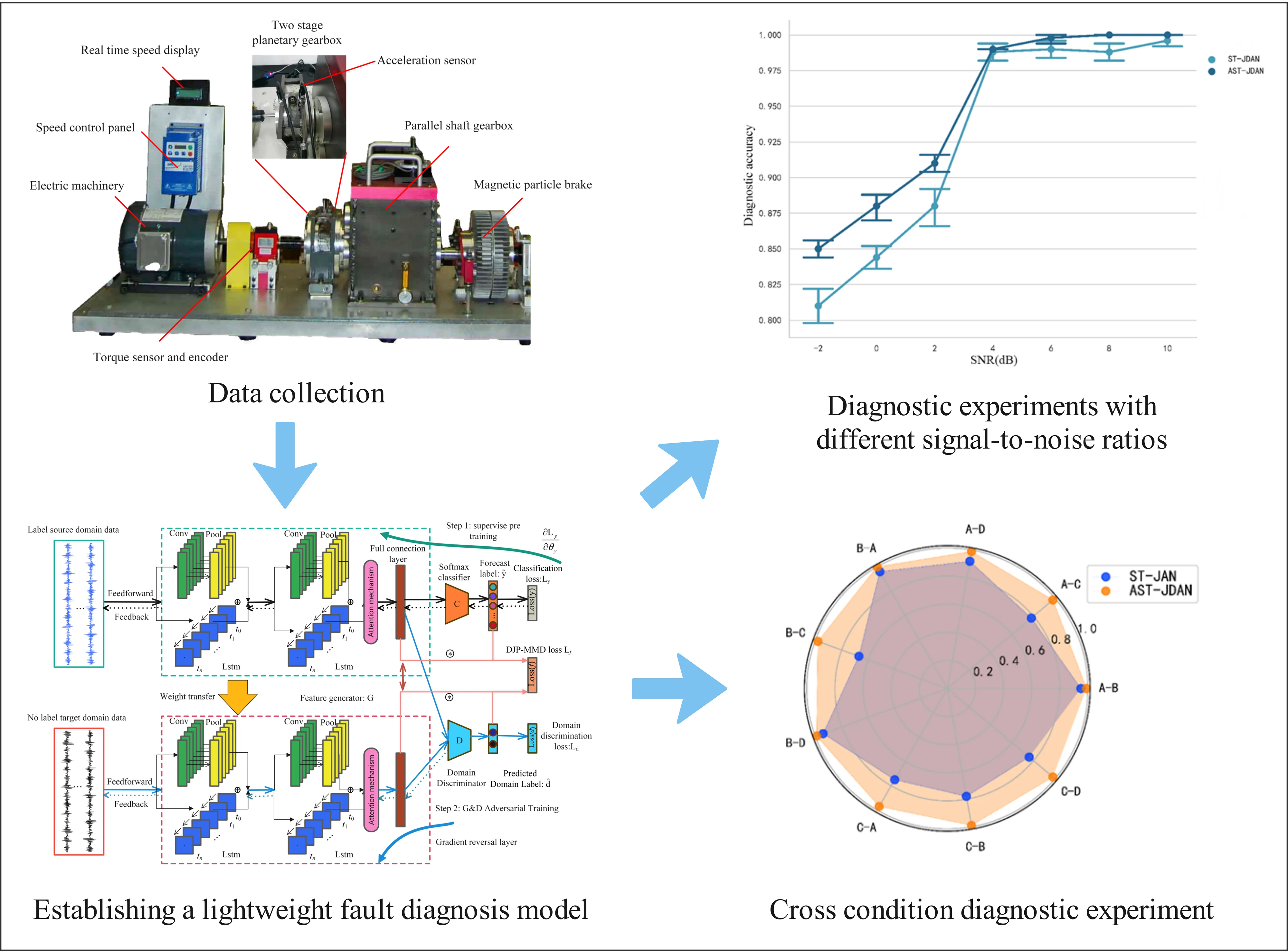
This article proposes a novel lightweight attention spatiotemporal joint distribution adaptation network fault diagnosis model to address the key challenges of domain transfer and high model complexity in traditional methods. The novelty lies in 1. Using model compression techniques to reduce the complexity of the network model and improve its computational efficiency; 2. Introducing new domain adaptation and adversarial methods to solve the domain transfer problem. The effectiveness of the proposed model is verified through a transfer experiment of planetary gearbox vibration data. The experimental results show that the proposed model reduces the parameters and computational complexity to 18 % and 15 % of the original model, respectively, and has a diagnostic accuracy of over 98 % in cross-condition transfer tasks, and still maintains an accuracy of over 88 % even under high noise levels. This indicates that the proposed model is an efficient and accurate fault diagnosis model.

A lightweight fault diagnosis model for planetary gearbox using domain adaptation and model compression

Highlights

Efficient Model Compression: The research introduces novel model compression techniques, reducing network complexity to 18% of the original, enhancing computational efficiency without compromising diagnostic accuracy.
Effective Domain Adaptation: By incorporating new domain adaptation and adversarial methods, the model successfully addresses domain transfer challenges, demonstrating a diagnostic accuracy of over 98% in cross-condition transfer tasks.
Robust Performance: The proposed fault diagnosis model maintains high accuracy (88%) even under challenging conditions with high noise levels, showcasing its robustness and effectiveness in real-world scenarios.

1. Introduction

Bearing, gear and other rotating mechanical parts are the parts with the highest failure rate in mechanical equipment. Timely fault diagnosis of rotating mechanical parts can ensure the safe and stable operation of mechanical equipment and avoid economic losses caused by failures.

The traditional mechanical fault diagnosis method mainly consists of two steps: artificial feature extraction and artificial pattern recognition. That is, first, manually extract the feature map that is easier to distinguish the fault type from the acoustic, optical, vibration acceleration, temperature and other signals, and then directly judge the fault type through the feature map. However, the method relying on artificial feature extraction is only applicable to situations where the complexity of the mechanical system dynamics model is low. In the case of high complexity, the features that can significantly represent the health state of the machine cannot be obtained, so it is not conducive to pattern recognition. In addition, in the case of high system complexity, the results of pattern recognition are easy to be affected by the subjective cognitive bias of experts, resulting in reduced accuracy of pattern recognition. The emergence of the machine learning (ML) method solves the problem of relying on artificial pattern recognition. After establishing the discrimination model, this method trains the parameters of the model through a large number of labeled data, so that the model can output the fault discrimination results, thus avoiding the risk of accuracy decline caused by subjective judgment. Fault diagnosis models based on traditional ML include support vector machine, decision tree, K nearest neighbor algorithm, etc. Li et al. [1] used a multi-core support vector machine to diagnose the fault of a gas turbine and verified the performance of the model through comparative experiments. For the structure of the model itself and the problem of computational efficiency, some scholars solve it by simplifying the model parameters and improving the algorithm for optimizing the model. For example, Vong et al. [2] extract features through wavelet packet transform. With the extracted features, the engine faults are then classified by a multi-class least squares support vector machine. Li et al. [3] used particle swarm optimization to improve the training process of SVM.

With the development of ML technology in recent years, intelligent fault diagnosis has also come into being. Among them, intelligent fault diagnosis based on deep learning (DL) solves the problem that the feature extraction of traditional machine fault diagnosis depends on the prior knowledge of experts. The DL model can automatically extract more complete fault features for classification. To lower the model's complexity, many scholars first use traditional feature transformation to extract shallow features from the original data, and then use DL technology to extract deep-level features and conduct pattern recognition [4]. Fault diagnosis methods based on DL often use convolutional neural networks [5] (CNN), recurrent neural networks [6] (RNN), generative adversarial networks [7] (GAN), deep belief networks [8] (DBN), stacked autoencoders [9] (SAE) and other models. Islam et al. [4] collected the signal of the bearing through the acoustic transmitter, converted the information into wavelet spectrum by wavelet packet transform, then selected the band signal with significant characteristics through the defect rate index, and finally input the band signal into the adaptive CNN to diagnose the fault. Demetgul et al. [10] used Diffusion Maps, Local Linear Embedding, and AutoEncoders for feature extraction, and used Gustafson-Kessel and k-medoids algorithms to classify encoded signals, achieving good diagnostic accuracy in fault diagnosis of material handling systems. Zhang et al. [11] supplement-ed the original data set through Gan to make the sample categories balanced, and then used CNN model for feature extraction and pattern recognition. Through comparative experiments, it was proved that the fault diagnosis effect of this approach is better than that of the approach without data expansion. Zhao et al. [12] proposed a deep branch attention network, which can flexibly integrate vibration and velocity information to obtain higher diagnostic accuracy.

The premise of the application of the above fault diagnosis method is that the training samples and the test samples are independent and identically distributed in the probability distribution. However, in the actual situation, the probability distribution of the machine state data is often different due to different working conditions. The distribution difference between training data and test data will cause a domain confrontation phenomenon [13], which will greatly reduce the model diagnosis accuracy. Therefore, it is necessary to introduce domain adaptation into fault diagnosis methods to solve the problem of domain offset. In many industrial contexts, it is challenging to collect labeled data for practical applications, while it is simpler to collect non-labeled data. Based on this, this paper will realize the mapping of the original data to the machine health state under variable conditions through unsupervised deep domain adaptive transfer learning (TL) method, that is, build an end-to-end model, and train the model through labeled source domain data and unlabeled target domain data. TL-based intelligent fault methods have received a lot of attention recently. Te et al. [14] used convolutional neural networks as feature extractors and classifiers, and added domain classifiers to the model. Through confrontation training, the feature extractors can extract common features of the two domains, and finally conduct fault diagnosis through the classifier. Xu et al. [15] obtained the simulation fault data of the workshop through the data twin technology, and then realized the fault diagnosis of the actual workshop through the simulation fault data and the improved sparse stacking automatic encoder.

The general approximation theorem points out that a multilayer feedforward network containing enough hidden layer neurons can approximate any continuous function with any accuracy. However, the development direction of DL model is always towards the trend of more layers and larger width scales. Due to the limitation of hardware on computing power, the number of hidden layer neurons and network layers will be limited, while simply increasing the network depth of the model will increase the risk of gradient cliff or gradient explosion. At the same time, the computational efficiency of the huge model is low, which is not conducive to real-time fault diagnosis. In order to enhance the capability of feature extraction and pattern discrimination under limited model parameters, it is necessary to optimize the model parameters and computational complexity. The technology of model compression and accelerated depth neural network has been continuously developed in recent years, and is widely used to reduce the parameter amount and calculation amount of the model. This technology can be divided into parameter pruning and quantization, low-rank decomposition, transfer/compact convolution filter and knowledge distillation [16]. For the traditional DL-based fault diagnosis technology, there are problems of accuracy drop caused by domain offset and redundancy of model parameters and computation.

This paper aims at the problem of domain confrontation and the redundancy of model parameters and computation in the DL fault diagnosis method. This paper proposes a spatio-temporal neural network (STN) based on convolutional neural network (CNN) and long short memory network (LSTM). On the basis of STN, attention mechanism (AM) is introduced to enhance the significance of extracted features. Then domain adaptation and domain confrontation mechanism are introduced to strengthen the robustness of fault diagnosis under different working conditions. Finally, a lightweight attention spatio-temporal network fusion joint distribution domain adaptation (AST-JDAN) fault diagnosis model is obtained through model compression technology.

2. Theoretical background

2.1. Soft attention mechanism

The purpose of AM is to enable each feature vector to obtain the similarity between features, so that similar features can obtain more significant feature interaction, and finally enable the model to extract more significant fault features to promote fault diagnosis.

Fig. 1Wayne diagram of AM classification [17]

The AM can be broken down into channel attention, space attention, time attention, space-time attention, space channel attention, and branch attention, as shown in Fig. 1. This paper mainly deals with spatial AM. Spatial AM is divided into soft AM and hard AM according to the weight of selected fault eigenvalue. The soft AM takes each feature into account, and the weight of each feature is between 0 and 1, while the hard AM only selects the features that have a large relationship. The weight of the features that have a large relationship is 1, and the weight of the features that have a small relationship is 0. Because the hard AM excludes the features of small relationship, it may lead to information omission and affect the fault diagnosis accuracy of the model, so this paper selects the soft AM.

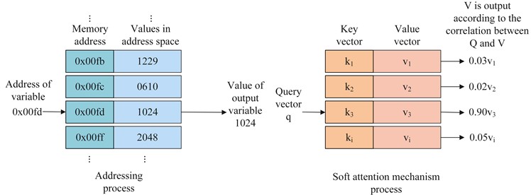
As shown in Fig. 2, the hard AM is like an addressing process, which finds the value stored in the address space through a fixed address, while the soft AM is similar to the soft addressing process. The difference from the hard AM is that each time the query vector matches a key value pair, $v$ will be output, and the proportion of the output depends on the degree of correlation between the query vector and the key vector. In the hard AM, it is believed that each time the key value pair is matched, it is either 100 % related or irrelevant.

The output features through the soft AM are mainly divided into the following steps: (1) Prepare the query vector $q$ , the key vector $k$ , and the value vector $v$ . In this fault diagnosis model, $q$ is the feature of the last time step of LSTM layer output in STN, $k$ and $v$ are the output of each time step of LSTM and the output of each channel of convolution layer. (2) Calculate the score $s$ (also called attention distribution) of each characteristic $v$ , and weight $v$ output. The calculation formula of $s$ is shown in Eq. (1):

1

s_{i} = p (z = i| K, q) = S o f t m a x (s c o r e (k_{i}, q)), i = 1,2, . . ., N .

Among them, $s c o r e$ is a $s c o r e$ function to calculate the degree of correlation between the key vector and the query vector. The score function usually uses the dot product model, as shown in Eq. (2), that is, the dot product between vectors is calculated to represent the correlation between vectors. Obviously, when two vectors are orthogonal (independent), the scoring value is 0. The scaling point product model is shown in Eq. (3), which reduces $d^{1 / 2}$ based on the point product model, where $d$ is the dimension of input $k_{i}$ . Eq. (4) is a bilinear model, which introduces a trainable weight matrix $W$ on the basis of the point product model. The author Kim [18], who proposed the model, believes that the conventional point product model establishes a separate attention distribution for each category, ignoring the correlation between multiple categories of inputs. By introducing $W$ , the knowledge of attention distribution established by each category will be learned by $W$ , making contributions to the establishment of attention distribution of the next category. Wu [19]proposed an additive model, as shown in Eq. (5). Compared with the bilinear model, it increases the attention value $U_{q}$ of A global context awareness and is activated through the $t a n h$ function. Where, $W$ and $U$ are trainable weight matrices:

2

s c o r e (x_{i}, q) = x_{i}^{T} q,

3

s c o r e (x_{i}, q) = \frac{x_{i}^{T} q}{\sqrt{d}},

4

s c o r e (x_{i}, q) = x_{i}^{T} W q,

5

s c o r e (x_{i}, q) = v^{T} t a n h (W x_{i} + U q) .

After obtaining the attention distribution $s$ , let $k = v$ , and obtain the output value of the AM lay er through weighted summation, as shown in Eq. (6):

6

a t t (X, q) = \sum_{i = 1}^{N} s_{i} v_{i} = \sum_{i = 1}^{N} s_{i} k_{i} .

2.2. Domain countermeasure mechanism

Ganin et al. [20] introduced the domain confrontation learning mechanism in the deep neural network in 2016, and proposed the domain adversarial neural network (DANN). DANN consists of three networks, including feature extractor ( $G_{f}$ ), classifier ( $G_{y}$ ) and domain discriminator ( $G_{d}$ ). The function of feature extractor is to extract the features of source domain and target domain; The function of the classifier is to classify features; The function of the domain discriminator is to distinguish whether the features produced by the feature extractor come from source domain data or target domain data as much as possible.

Fig. 2Comparison of addressing process and soft AM process

The training goal of DANN is to enable the classifier to accurately classify the source domain features and make the domain discriminator unable to distinguish whether the features produced by the feature extractor come from the source domain data or the target domain data. In this way, the source domain and target domain can be mapped to the same feature space, the distribution between the two domains can be aligned, and then the target domain data can be classified through a classifier. The objective function expression of confrontation training is shown in Eq. (7):

7

\begin{matrix} \underset{y}{m i n} \underset{d}{m a x} L (y, d) = \sum_{i = 1}^{N} L_{y} (G_{y} (G_{f} (x_{i}; θ_{f}); θ_{y}), y_{i}) + \sum_{i = 1}^{N} L_{d} (G_{d} (R_{λ} (G_{f} (x_{i}; θ_{f})); θ_{d}), d_{i}), \end{matrix}

where, $N$ is the number of samples, $x_{i}$ is the input sample, $y_{i}$ is the sample label, $d_{i}$ is the domain label, $θ_{f}$ , $θ_{y}$ and $θ_{d}$ is the weight matrix of $G_{f}$ , $G_{y}$ and $G_{d}$ respectively, $L_{y}$ is the cross entropy loss function of class discrimination, $L_{d}$ is the cross entropy loss function of domain discrimination, $R_{λ}$ is a gradient inversion layer function, which keeps the independent variable output during feedforward propagation unchanged, while the gradient of the independent variable during backpropagation becomes the original - $λ$ times.

2.3. Model compression technology

The enormous model's poor computational efficiency makes it difficult to diagnose faults in real time, necessitating the optimization of model parameters and computing. The DL model compression theory has been developed recently.

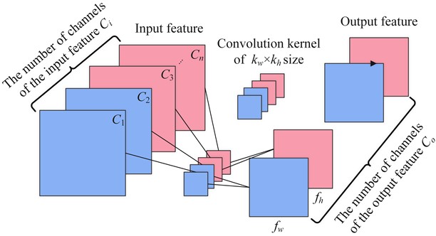
MobileNet [21] proposed by Google is an efficient model compression algorithm. Its core innovation is to replace the original convolution layer with depth separable convolution, which can achieve the same pattern recognition effect as the original model while reducing the number of model parameters and calculations. Depth separable convolution decomposes ordinary convolution operations into channel by channel convolution (DW) and point by point convolution (PW) [22]. The calculation process of ordinary convolution and depth separable convolution is shown in Fig. 3.

The upper part of Fig. 3 is a general convolution process. Each filter consists of several convolution cores. The quantity of channels in the output feature is the same as the quantity of filters. The parameter quantities (params) and calculation quantities (FLOPs) of the general convolution are shown in Eq. (8) and Eq. (9):

8

p a r a m s = C_{i} \cdot k_{w} \cdot k_{h} \cdot C_{o},

9

F L O P s = C_{o} \cdot f_{w} \cdot f_{h} \cdot C_{i} \cdot k_{w} \cdot k_{h},

where $C_{o}$ is the number of filters, $C_{i}$ is the number of convolution kernels for each filter, $k_{w}$ is the width of the convolution kernel, $k_{h}$ is the height of the convolution kernel, $f_{w}$ is the width of the output feature map, and $f_{h}$ is the height of the output feature map.

Fig. 3Comparison between ordinary convolution and deep separable convolution

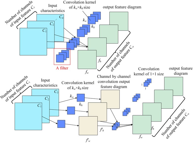
The depth separable convolution integrates the ordinary convolution into two stages, first channel by channel convolution (DW), and then point by point convolution (PW). In DW, $C_{i} =$ 1, $k_{w} =$ 1, $k_{h} =$ 1, and other parameters of ordinary convolution are the same. Combining Eq. (8), Eq. (9) and adding the parameter quantities and calculation quantities of DW and PW respectively, we can get the parameter quantities and calculation quantity formulas of depth separable convolution:

10

p a r a m s = C_{i} \cdot k_{w} \cdot k_{h} \cdot 1 + C_{i} \cdot 1 \cdot 1 \cdot C_{o} = C_{i} \cdot (k_{w} \cdot k_{h} + C_{o}),

11

\begin{matrix} F L O P s = 1 \cdot f_{w} \cdot f_{h} \cdot C_{i} \cdot k_{w} \cdot k_{h} + C_{o} \cdot f {}_{w} \cdot f_{h} \cdot C_{i} \cdot 1 \cdot 1 = f_{w} \cdot f_{h} \cdot C_{i} \cdot (k_{w} \cdot k_{h} + C_{o}) . \end{matrix}

GhostNet [23] proposed by Huawei Noah Lab is also one of the efficient compression model algorithms. It replaces the feature map generated by the original part of the convolution through an operation that saves the number of parameters and computation, thereby saving hardware resources. The feature map is called the ghost feature map. The process of generating the phantom feature map is shown in Fig. 4.

If the number of channels generated by the low-cost operation is $C_{p}$ , the phantom feature map matrix generated by each channel can be represented by Eq. (12):

12

(f_{o p})_{j} = φ_{j} (f_{i}), i = 1,2, . . ., C_{p}, j = 1,2, 3, . . ., C_{o} - C_{p},

where, $f_{i}$ is the feature map generated by ordinary convolution of the $i$ th sheet. If ordinary convolution is used to generate the feature map of $C_{p}$ sheet, $j$ low-cost operations are performed $φ_{j}$ Generate $C_{o}$ - $C_{p}$ phantom feature map $f_{o p}$ . In order to save computing resources, it is required that $C_{o} - C_{p} \geq C_{p}$ .

In this paper, packet convolution is selected as a low-cost operation, and the schematic diagram of packet convolution is shown in Fig. 5. Grouped convolution divides the channels of the input feature into g groups, and the number of convolution cores of the filter is the same as the number of channels of the input feature $C_{i}$ . Therefore, each filter should also divide the convolution cores into $g$ groups, and each group should perform convolution operations separately. Finally, all the feature maps output by the filter are spliced according to the channel dimensions. The formula for the number of parameters and calculation amount is shown in Eq. (13) and Eq. (14):

13

\begin{matrix} p a r a m s = (\frac{C_{i}}{g} \cdot k_{w} \cdot k_{h}) \cdot \frac{C_{o}}{g} \cdot g = \frac{C_{i} \cdot k_{w} \cdot k_{h} \cdot C_{o}}{g}, \end{matrix}

14

\begin{matrix} F L O P s = (\frac{C_{o}}{g} \cdot f_{w} \cdot f_{h}) \cdot (\frac{C_{i}}{g} \cdot k_{w} \cdot k_{h}) \cdot g = \frac{C_{o} \cdot f_{w} \cdot f_{h} \cdot C_{i} \cdot k_{w} \cdot k_{h}}{g} . \end{matrix}

It can be seen from Eq. (13) and Eq. (14) that the parameter amount and calculation amount of the packet convolution are 1/ $g$ of the ordinary convolution. It can be seen that the packet convolution is a cheaper operation than the ordinary convolution.

Fig. 4Convolution diagram of GhostNet

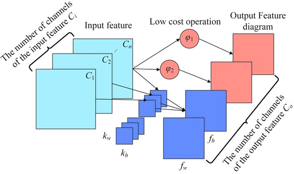
Fig. 5Schematic diagram of grouping convolution

2.4. Fusion domain adaptive fault diagnosis model based on lightweight spatio-temporal attention network

First, the soft AM is introduced into the end of the feature generator of the spatio-temporal neural network based on feature transfer learning (ST-JAN) [24], so that the network model can extract more significant fault features. Secondly, the domain confrontation mechanism is introduced to further migrate, so that the diagnosis model has better cross domain fault diagnosis capability. Finally, the model compression technology in MobileNet and GhostNet is introduced to reduce the parameter amount and calculation amount of the convolution layer in the diagnostic model and improve the calculation efficiency. Fig. 6 shows the architecture of AST-JDAN. The parameter settings of AST-JDAN are shown in Table 1.

Fig. 6Fusion domain adaptive fault diagnosis model based on spatio-temporal attention network

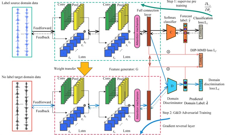
Table 1Model parameters of ASTN-JDAN.

Network layer type		Kernel size	Number of hidden units	Step size	Output tensor shape
ASTN feature generator	Input	*	*	*	(N,1,1024)
	Conv1d(1)	64	*	1	(N,16,963)
	BatchNorm1d(1)	*	*	*	(N,16,963)
	MaxPool1d(1)	3	*	2	(N,16,482)
	LSTM(1)	64	482	*	(N,16,482)
	Conv1d(2)	3	*	1	(N,32,482)
	BatchNorm1d (2)	*	*	*	(N,32,482)
	AdaptiveMaxPool1d	*	*	*	(N,32,30)
	LSTM(2)	15	30	*	(N,32,30)
	Attention mechanism layer	*	256	*	(N,256)
Fault category discriminator	Linear(1)	*	256	*	(N,256)
	Linear(2)	*	128	*	(N,256)
	Fault classifier	*	10	*	(N,10)
Domain discriminator	Gradient reversal layer	*	*	*	(N,256)
	Linear(3)	*	256	*	(N,256)
	Linear(4)	*	256	*	(N,128)
	Linear(5)	*	2	*	(N,2)

According to the relevant formula in Section 2.3, the parameter quantity and calculation quantity of the original convolution layer, as well as the parameter quantity and calculation quantity of the convolution layer after model compression can be calculated. Table 2 presents the outcomes. It can be seen from Table 2 that the parameters of the improved convolution layer are compressed from the original 2560 to 464, about 18 % of the original, while the calculated FLOPs are compressed from the original 1726464 to 262128, about 15 % of the original.

Table 2Comparison of parameters of convolutional layers after model compression

Convolutional layer	Ordinary convolution 1	Ordinary convolution 2	Depthwise separable convolution 1	Grouped convolution 2
Number of input channels $C_{i}$	1	16	1	16
Convolution kernel size $k_{w} * k_{h}$	1*64	3	1*64	3
Number of output channels C_o	16	32	16	32
Output feature Size $f_{w} * f_{h}$	1*963	1*482	1*963	1*482
Parameter quantity params	1024	1536	80	384
Amount of computation FLOPs	986112	740352	77040	185088
Total amount of parameters	2560		464
Total calculation amount	1726464		262128

3. Fault diagnosis test of secondary planetary gearbox

3.1. Introduction to DDS experimental platform

The experimental data comes from the vibration signals of the secondary planetary gearbox collected on the Drivetrain Diagnostics Simulator (DDS) test bench, as shown in Fig. 7. The test-bed can simulate the wear, crack, broken tooth and missing tooth faults of straight and helical gears, as well as the faults of inner ring, outer ring and rolling element of rolling bearings. Different working conditions can be simulated by setting different speeds and loading different torsional loads. DDS test bench is mainly composed of power module, spindle module and brake. In the power module, the variable speed drive motor provides power. The speed control panel controls the motor speed. The torque sensor and encoder are used to collect the torque and detect the pulse signal generated by the speed. The real-time display displays the actual speed. Because of the slip and other factors in gear transmission, the set speed is often slightly lower than the actual speed. The main shaft module mainly includes the main shaft, parallel gearbox and secondary planetary gearbox. In addition, an acceleration sensor is installed on the gearbox to collect fault vibration signals. The programmable magnetic powder brake at the end of the test bench is used to control the load of the spindle and simulate the rotation under different loads.

In this experiment, the fault gear of the secondary planetary gearbox is set on the sun gear, and there are four fault types in total, namely, missing tooth, broken tooth, surface wear and tooth root crack, as shown in Fig. 8. In addition, the gear is normal, and there are five health conditions for the gear.

3.2. Test data collection

The sampling frequency set in the experiment is 12.8 kHz. The motor has two rotation frequencies of 20 Hz and 30 Hz, and the load current size is 0.4 A and 0.8 A. Therefore, the experiment has four working conditions: 20 Hz 0.4 A, 20 Hz 0.8 A, 30 Hz 0.4 A and 30 Hz 0.8 A. The four working conditions are named as A, B, C and D. Each working condition has five health conditions of gears: normal, missing, broken, surface wear and tooth root crack. Through the statistics of each original data file, it can be found that the number of samples of each type under each working condition is consistent, and the data volume is sufficient, reaching 1048548 data points, without data imbalance. Therefore, sufficient samples can be directly collected by non-overlapping sampling, that is, the sampling step is equal to the sample length $n =$ 1024. The expression of the total sample size $M$ is shown in Eq. (15), where the constant 5 represents the data of five machine health states, and $l =$ 1048548 is the length of each type of data. The total sample size under each working condition is obtained by Eq. (15), as shown in Table 3:

15

M = 5 \times ⌊\frac{l}{n}⌋ .

Table 3Data length and sampling quantity of DDS test bench planetary gearbox under each working condition

No.	Working condition	Health condition	Data size	Sample size	Total sample size
A	20 Hz 0.4 A	Normal	1048548	1023	5115
		Missing teeth	1048548	1023
		Broken teeth	1048548	1023
		Surface wear	1048548	1023
		Root crack	1048548	1023
B	20 Hz 0.8 A	Normal	1048548	1023	5115
		Missing teeth	1048548	1023
		Broken teeth	1048548	1023
		Surface wear	1048548	1023
		Root crack	1048548	1023
C	30 Hz 0.4 A	Normal	1048548	1023	5115
		Missing teeth	1048548	1023
		Broken teeth	1048548	1023
		Surface wear	1048548	1023
		Root crack	1048548	1023
D	30 Hz 0.8 A	Normal	1048548	1023	5115
		Missing teeth	1048548	1023
		Broken teeth	1048548	1023
		Surface wear	1048548	1023
		Root crack	1048548	1023

Fig. 7Drivetrain diagnostics simulator test bench

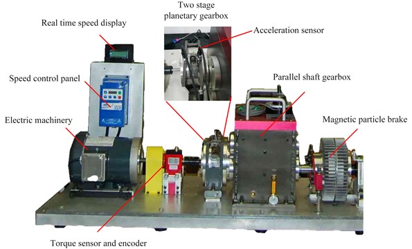
Fig. 9 shows two samples of CWRU fault bearing data set and DDS planetary gearbox data set. The blue part of Fig. 9(a) and Fig. 9(b) is the original vibration signal, and the red part is the envelope of the original vibration signal. Then, the envelope spectrum of the signal is obtained through the envelope line of fast Fourier transform, as shown in Fig. 9(c) and Fig. 9(d). It is not difficult to find that the sideband spectrum of the planetary gearbox is more complex from the spectrum diagram, which indicates that the fault diagnosis of the planetary gearbox signal of the DDS test bench is more difficult. This is a greater challenge for the transfer task of the model.

Fig. 8Machining simulation of four kinds of gear faults

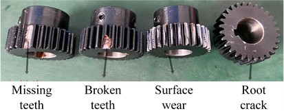
Fig. 9Comparison of envelope spectra of bearing data and planetary gearbox data

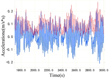
a) Original vibration signal of rolling bearing

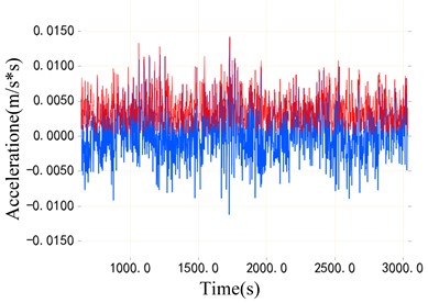
b) Original vibration signal of planetary gearbox

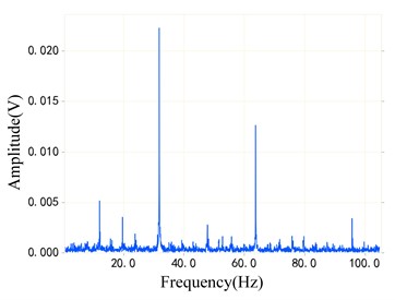
c) Rolling bearing envelope spectrum

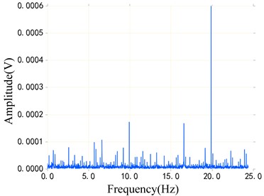
d) Planetary gearbox envelope spectrum

3.3. The influence of attention mechanism

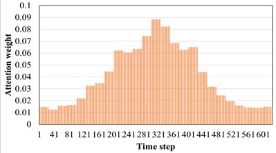
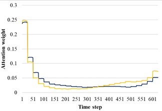
The AM introduced earlier can adaptively screen out the favorable features for machine fault diagnosis tasks. Therefore, in the soft AM, each part can be given different weights as the realization form of soft screening. The model used in this section is AST-JDAN fault diagnosis model. The working condition of source domain data is 20 Hz 0.4 A, and that of target domain data is 20 Hz 0.8 A. The AST-JDAN model is trained with source domain data, and then the attention weight distribution of different health state data is extracted from it, as shown in Fig. 10. The distribution of attention weight can reflect the degree of attention paid to different time steps. It can be seen from Fig. 10 that data in different health states have significantly different attention distribution rules. For tooth breakage fault, the attention distribution is mainly concentrated on the later time step, and slightly concentrated in the middle, which is similar to the attention distribution of surface wear fault, but the latter distribution is more concentrated on the later time step, and the weight value in the middle is smaller. The attention distribution of missing teeth fault and gear normal is close to the forward time step, but the attention distribution of gear normal is more concentrated on the left side, and the weight value in the middle is smaller; The attention of the crack fault is concentrated in the middle of the time step, and gradually decreases at both ends.

Fig. 10Attention distribution diagram of different sun wheel health states

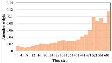
a) Broken teeth

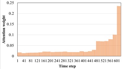
b) Surface wear

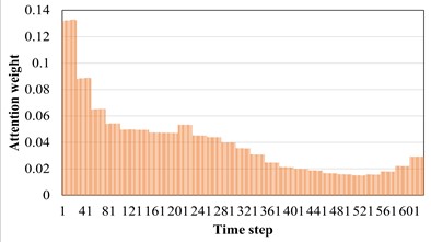
c) Missing teeth

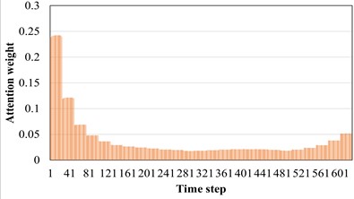
d) Normal

e) Root crack

In order to reveal the influence of attention distribution in the transfer process, the source domain and target domain are input into the trained AST-JDAN model, and the extracted attention distribution is shown in Fig. 11. The yellow line represents the attention weight distribution diagram of the source domain data, and the blue line represents the attention weight distribution diagram of the target domain data. It can be seen from Fig. 11 that data with the same health status in different domains have generally similar attention weight distribution, which enables the AM in the target domain to enhance the features conducive to pattern recognition.

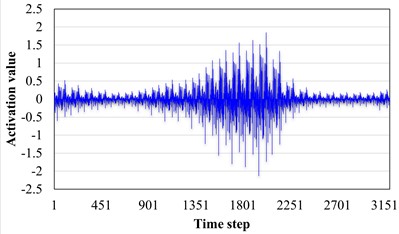
In order to explore the influence of AM layer on pattern recognition, the target field tooth break fault data and crack fault data are input to the trained AST-JDAN, and their output features are spliced and visualized through channels. The results are shown in Fig. 12. It can be seen from Fig. 12 that the output characteristics of two different fault category data before the AM layer are similar, showing similar periodic pulses. Through careful observation, it can be seen that the activation value of the feature output of the broken tooth fault shows a trend of gradually decreasing on both sides of the middle high, similar to a spindle. However, the crack fault shows a tendency for the two sides of the middle concave bulge first and then decrease. This small difference is difficult for the classifier to classify. After the AM layer, the characteristics of the middle part of the tooth fracture data are enhanced, while the characteristics of the two sides are relatively weakened, making the overall shape of the features more easily distinguishable. At the same time, the characteristics of the two peaks of the crack fault are also more significantly changed, which verifies the ability of the AM to enhance the data characteristics.

Fig. 11Attention distribution of different sun wheel health states in source domain and target domain

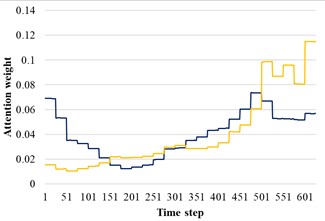
a) Broken teeth

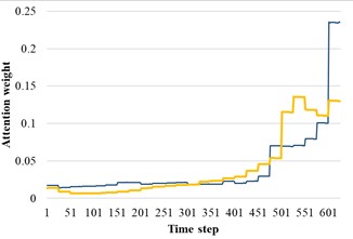
b) Surface wear

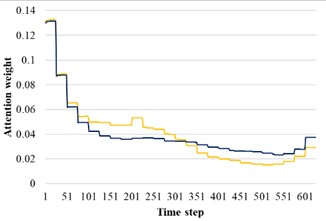
c) Missing teeth

d) Normal

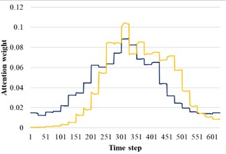
e) Root crack

3.4. Model diagnosis results and analysis

The influence of AM is verified by comparing transfer fault diagnosis experiments between different loads. The radar chart shown in Fig. 13 is a comparison of the transfer accuracy of AST-JDAN and ST-JAN under different working conditions. It can be seen from the Fig. 13 that under the transfer tasks of B-A, A-B and B-D, ST-JAN and AST-JDAN have achieved high fault diagnosis accuracy, higher than 94 %. However, the fault diagnosis accuracy of ST-JAN in the transfer tasks of A-C, A-D, B-C, C-A, C-B, C-D is significantly lower than that of AST-JDAN. The reason is that the AM can enable the model to enhance the significance of the features that are beneficial to the transfer task, making it easier for the classifier to diagnose faults. Secondly, AST-JDAN integrates domain countermeasure method in ST-JAN domain adaptation method, which enables feature generator to better extract domain invariant features.

Fig. 12Change diagram of fault characteristics of broken teeth and cracks in the target domain

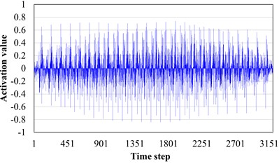
a) Fault characteristics of broken teeth

b) Fault characteristics of broken teeth passing through the attention layer

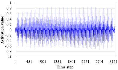
c) Fault characteristics of crack

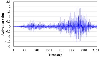
d) Fault characteristics of crack passing through the attention layer

Fig. 13Transfer diagnosis accuracy of ST-JAN and AST-JDAN under different loads

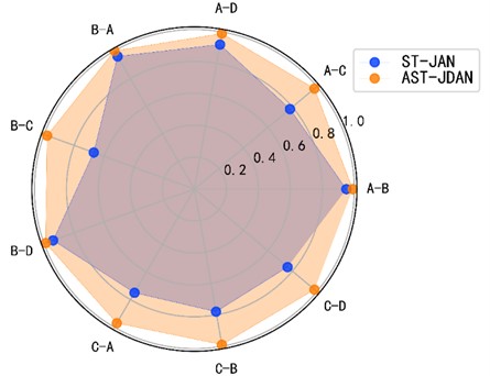
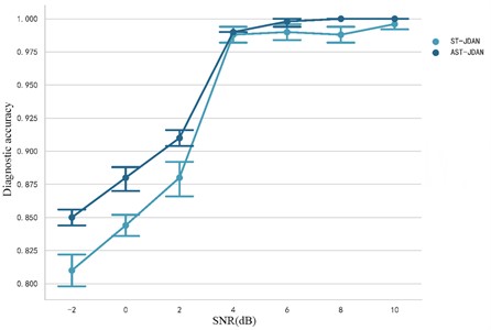
Fig. 14 shows the comparison of fault diagnosis accuracy between ST-JDAN without AM and AST-JDAN with AM under different noise intensities in transfer tasks A-B. It can be seen from the experimental data that the average fault diagnosis accuracy of AST-JDAN is about 3 %-4 % higher than that of ST-JDAN in the case of high noise intensity, but the average fault diagnosis accuracy of AST-JDAN is not significantly improved in the case of low noise intensity. The experimental results show that the AM can enable the model to extract more significant fault features, and improve the problem that features are not obvious due to the submergence of features under strong noise.

Fig. 14Precision comparison between ST-JAN and AST-JDAN under different signal-to-noise ratios

4. Conclusions

In this paper, AST-JDAN is established. This model solves the problem of domain offset through fusion domain adaptation and domain confrontation methods. Model compression technology reduces the complexity of the model and improves the computational efficiency. The validity of the proposed model is verified by the vibration signal data set of the planetary gearbox. The results suggest that the model can obtain higher fault diagnosis accuracy in cross domain fault diagnosis, and the model has higher diagnosis accuracy than other models under strong noise interference.

This article is dedicated to the fault diagnosis of rotating machinery using deep transfer learning under variable operating conditions, but its diagnostic effectiveness depends on a large amount of annotated fault data. If fault data is scarce, the diagnostic accuracy will be greatly affected. In recent years, digital twin technology has developed rapidly. Through digital twin technology, fault data of mechanical equipment to be diagnosed can be obtained, providing a solution to the problem of scarce fault data. In the future, we will further research fault diagnosis methods that combine digital twin technology with transfer learning.

References

Z. Li, S.-S. Zhong, and L. Lin, “Novel gas turbine fault diagnosis method based on performance deviation model,” Journal of Propulsion and Power, Vol. 33, No. 3, pp. 730–739, May 2017, https://doi.org/10.2514/1.b36267

Publisher
C. M. Vong and P. K. Wong, “Engine ignition signal diagnosis with wavelet packet transform and multi-class least squares support vector machines,” Expert Systems with Applications, Vol. 38, No. 7, pp. 8563–8570, Jul. 2011, https://doi.org/10.1016/j.eswa.2011.01.058

Publisher
Y. Li, B. Miao, W. Zhang, P. Chen, J. Liu, and X. Jiang, “Refined composite multiscale fuzzy entropy: Localized defect detection of rolling element bearing,” Journal of Mechanical Science and Technology, Vol. 33, No. 1, pp. 109–120, Jan. 2019, https://doi.org/10.1007/s12206-018-1211-8

Publisher
M. M. M. Islam and J.-M. Kim, “Automated bearing fault diagnosis scheme using 2D representation of wavelet packet transform and deep convolutional neural network,” Computers in Industry, Vol. 106, pp. 142–153, Apr. 2019, https://doi.org/10.1016/j.compind.2019.01.008

Publisher
L. Chen, K. An, D. Huang, X. Wang, M. Xia, and S. Lu, “Noise-boosted convolutional neural network for edge-based motor fault diagnosis with limited samples,” IEEE Transactions on Industrial Informatics, Vol. 19, No. 9, pp. 9491–9502, Sep. 2023, https://doi.org/10.1109/tii.2022.3228902

Publisher
Y. Liu, R. Young, and B. Jafarpour, “Long-short-term memory encoder-decoder with regularized hidden dynamics for fault detection in industrial processes,” Journal of Process Control, Vol. 124, pp. 166–178, Apr. 2023, https://doi.org/10.1016/j.jprocont.2023.01.015

Publisher
H. Shao, W. Li, B. Cai, J. Wan, Y. Xiao, and S. Yan, “Dual-threshold attention-guided GAN and limited infrared thermal images for rotating machinery fault diagnosis under speed fluctuation,” IEEE Transactions on Industrial Informatics, Vol. 19, No. 9, pp. 9933–9942, Sep. 2023, https://doi.org/10.1109/tii.2022.3232766

Publisher
G. Yuan, Z. Liang, Z. Jiawei, W. Bojia, and Y. Zhongchao, “Research on reliability of centrifugal compressor unit based on dynamic Bayesian network of fault tree mapping,” Journal of Mechanical Science and Technology, Vol. 37, No. 5, pp. 2667–2677, May 2023, https://doi.org/10.1007/s12206-023-0440-7

Publisher
X. Yan, W. Liang, G. Zhang, B. She, and F. Tian, “Fault diagnosis method for complex feeding and ramming mechanisms based on SAE-ACGANs with unbalanced limited training data,” Journal of Vibration and Shock, Vol. 42, No. 2, pp. 89–99, Jan. 2023.

Search CrossRef
M. Demetgul, K. Yildiz, S. Taskin, I. N. Tansel, and O. Yazicioglu, “Fault diagnosis on material handling system using feature selection and data mining techniques,” Measurement, Vol. 55, pp. 15–24, Sep. 2014, https://doi.org/10.1016/j.measurement.2014.04.037

Publisher
W. Zhang, X. Li, X.-D. Jia, H. Ma, Z. Luo, and X. Li, “Machinery fault diagnosis with imbalanced data using deep generative adversarial networks,” Measurement, Vol. 152, p. 107377, Feb. 2020, https://doi.org/10.1016/j.measurement.2019.107377

Publisher
D. Zhao, S. Liu, H. Du, L. Wang, and Z. Miao, “Deep branch attention network and extreme multi-scale entropy based single vibration signal-driven variable speed fault diagnosis scheme for rolling bearing,” Advanced Engineering Informatics, Vol. 55, p. 101844, Jan. 2023, https://doi.org/10.1016/j.aei.2022.101844

Publisher
K. Weiss, T. M. Khoshgoftaar, and D. Wang, “A survey of transfer learning,” Journal of Big Data, Vol. 3, No. 1, pp. 1–40, Dec. 2016, https://doi.org/10.1186/s40537-016-0043-6

Publisher
T. Han, C. Liu, W. Yang, and D. Jiang, “A novel adversarial learning framework in deep convolutional neural network for intelligent diagnosis of mechanical faults,” Knowledge-Based Systems, Vol. 165, pp. 474–487, Feb. 2019, https://doi.org/10.1016/j.knosys.2018.12.019

Publisher
Y. Xu, Y. Sun, X. Liu, and Y. Zheng, “A digital-twin-assisted fault diagnosis using deep transfer learning,” IEEE Access, Vol. 7, pp. 19990–19999, 2019, https://doi.org/10.1109/access.2018.2890566

Publisher
Y. Cheng, D. Wang, P. Zhou, and T. Zhang, “Model compression and acceleration for deep neural networks: The principles, progress, and challenges,” IEEE Signal Processing Magazine, Vol. 35, No. 1, pp. 126–136, Jan. 2018, https://doi.org/10.1109/msp.2017.2765695

Publisher
M.-H. Guo et al., “Attention mechanisms in computer vision: A survey,” Computational Visual Media, Vol. 8, No. 3, pp. 331–368, Sep. 2022, https://doi.org/10.1007/s41095-022-0271-y

Publisher
J.-H. Kim, J. Jun, and B.-T. Zhang, “Bilinear attention networks,” arXiv:1805.07932v2, 2018, https://doi.org/10.48550/arxiv.1805.07932

Publisher
C. Wu, F. Wu, T. Qi, Y. Huang, and X. Xie, “Fastformer: Additive attention can be all you need,” arXiv:2108.09084, 2021, https://doi.org/10.48550/arxiv.2108.09084

Publisher
Y. Ganin et al., “Domain-adversarial training of neural networks,” arXiv.1505.07818, 2015, https://doi.org/10.48550/arxiv.1505.07818

Publisher
A. G. Howard et al., “Mobilenets: Efficient convolutional neural networks for mobile vision applications,” arXiv:1704.04861, 2017, https://doi.org/10.48550/arxiv.1704.04861

Publisher
L. Luo, T. Zhu, G. Zhang, Q. Ding, and Z. Huang, “Building extraction from high-resolution remote sensing images based on deeplabv3+ model,” Electronic Information Countermeasure Technology, Vol. 36, No. 4, pp. 65–69, 2021.

Search CrossRef
K. Han, Y. Wang, Q. Tian, J. Guo, C. Xu, and C. Xu, “Ghostnet: More features from cheap operations,” in Proceedings of the IEEE/CVF conference on computer vision and pattern recognition, pp. 1580–1589, 2019, https://doi.org/10.48550/arxiv.1911.11907

Publisher
M. Song, Z. Zhang, S. Xiao, Z. Xiong, and M. Li, “Bearing fault diagnosis method using a spatio-temporal neural network based on feature transfer learning,” Measurement Science and Technology, Vol. 34, No. 1, p. 015119, Jan. 2023, https://doi.org/10.1088/1361-6501/ac9078

Publisher

About this article

Received

22 May 2023

Accepted

03 October 2023

Published

23 January 2024

SUBJECTS

Fault diagnosis based on vibration signal analysis

DOI

https://doi.org/10.21595/jve.2023.23412

Keywords

transfer learning

fault diagnosis

attention mechanism

model compression technology

Acknowledgements

This paper was supported by the following research projects: the Key Technology Innovation Project of Fujian Province (Grant no. 2022G02030), the Natural Science Foundation of Fujian Province (Grants no. 2022J011223), and Youth and the collaborative innovation center project of Ningde Normal University (Grant No. 2023ZX01).

Data Availability

The datasets generated during and/or analyzed during the current study are available from the corresponding author on reasonable request.

Author Contributions

Conceptualization, Mengmeng Song and Shungen Xiao; software, Zexiong Zhang; validation, Mengwei Li, Jihua Ren and Yaohong Tang; writing-original draft preparation, Zexiong Zhang; writing-review and editing, Zicheng Xiong.

Conflict of interest

The authors declare that they have no conflict of interest.

This is an open access article distributed under the Creative Commons Attribution License, which permits unrestricted use, distribution, and reproduction in any medium, provided the original work is properly cited.

Previous article in issue Previous Next article in issue Next

Review article

2023 11 04

A comprehensive review of mechanical fault diagnosis methods based on convolutional neural network

Junjian Hou, Xikang Lu, Yudong Zhong, Wenbin He, Dengfeng Zhao, Fang Zhou

Research article

2023 08 18

Fault diagnosis of rolling bearing based on cross-domain divergence alignment and intra-domain distribution alienation

Shubiao Zhao, Guangbin Wang, Xuejun Li, Jinhua Chen, Lingli Jiang

Research article

2023 08 01

A fault diagnosis method based on dilated convolution and attention for rolling bearing under multiple working conditions and noisy environments

Hui Zhang, Shengdong Liu, Ziwei Lv, Zhenlong Sang, Fangning Li

Research article

2022 06 30

A convolutional neural network method based on Adam optimizer with power-exponential learning rate for bearing fault diagnosis

Youming Wang, Zhao Xiao, Gongqing Cao

M. Song et al., “A lightweight fault diagnosis model for planetary gearbox using domain adaptation and model compression,” Journal of Vibroengineering, Vol. 26, No. 2, pp. 279–296, Jan. 2024, https://doi.org/10.21595/jve.2023.23412

Copy Extrica

Copied to clipboard!

TY  - JOUR
DO  - 10.21595/jve.2023.23412
UR  - https://doi.org/10.21595/jve.2023.23412
TI  - A lightweight fault diagnosis model for planetary gearbox using domain adaptation and model compression
T2  - Journal of Vibroengineering
AU  - Song, Mengmeng
AU  - Xiong, Zicheng
AU  - Zhang, Zexiong
AU  - Ren, Jihua
AU  - Li, Mengwei
AU  - Xiao, Shungen
AU  - Tang, Yaohong
PY  - 2024
DA  - 2024/01/23
PB  - Extrica
SP  - 279-296
VL  - 26
IS  - 2
SN  - 1392-8716
SN  - 2538-8460
ER  - 

Copy Ris

Copied to clipboard!

 @article{Song_2024, title={A lightweight fault diagnosis model for planetary gearbox using domain adaptation and model compression}, volume={26}, ISSN={2538-8460}, url={https://doi.org/10.21595/jve.2023.23412}, DOI={10.21595/jve.2023.23412}, number={2}, journal={Journal of Vibroengineering}, publisher={JVE International Ltd.}, author={Song, Mengmeng and Xiong, Zicheng and Zhang, Zexiong and Ren, Jihua and Li, Mengwei and Xiao, Shungen and Tang, Yaohong}, year={2024}, month=jan, pages={279–296} }

Copy Bibtex

Copied to clipboard!

[1]M. Song et al., “A lightweight fault diagnosis model for planetary gearbox using domain adaptation and model compression,” Journal of Vibroengineering, vol. 26, no. 2, pp. 279–296, Jan. 2024, doi: 10.21595/jve.2023.23412.

Copy IEEE

Copied to clipboard!

Song, Mengmeng, Zicheng Xiong, Zexiong Zhang, Jihua Ren, Mengwei Li, Shungen Xiao, and Yaohong Tang. “A Lightweight Fault Diagnosis Model for Planetary Gearbox Using Domain Adaptation and Model Compression.” Journal of Vibroengineering 26, no. 2 (January 23, 2024): 279–96. https://doi.org/10.21595/jve.2023.23412.

Copy Chicago

Copied to clipboard!

A lightweight fault diagnosis model for planetary gearbox using domain adaptation and model compression

Abstract

Highlights

1. Introduction

2. Theoretical background

2.1. Soft attention mechanism

2.2. Domain countermeasure mechanism

2.3. Model compression technology

2.4. Fusion domain adaptive fault diagnosis model based on lightweight spatio-temporal attention network

3. Fault diagnosis test of secondary planetary gearbox

3.1. Introduction to DDS experimental platform

3.2. Test data collection

3.3. The influence of attention mechanism

3.4. Model diagnosis results and analysis

4. Conclusions

References

About this article

Related Articles