Abstract
Population growth and rapid urban development have led to urbanization, caused environmental problems such as: heat islands and air pollution. The installation of park green space system is widely regarded as effective in alleviating the thermal environment and improving the surrounding air quality. Therefore, this study focuses on parks in highly developed cities, The measurements of terrain and topography were conducted using unmanned aerial vehicles (UAVs) to establish a terrain model. This model was combined with environmental factors such as wind speed, direction, solar radiation, temperature, and soil infiltration were measured to assess the correlation between different landscape elements and the environment in various parks. In addition, an air particulate monitor (Arduino Uno) was developed to measure the contribution of green space systems to urban air pollution. Furthermore, by integrating measurements of multiple factors and employing the Pearson's correlation method and three-dimensional scatter plots, this study explored the relationships between many variables of park. Test results show that 1. The materials of the landscape elements should have moderate thermal conductivity; 2. The moisture content of the soil of grassland should be monitored; 3. To improve the air quality, the correlation between wind speed and wind direction should be considered in the placement of landscape elements.
1. Introduction
A 2014 report from the United Nations noted that six-sevenths of the global population will live in urban areas by 2045. The population is gradually becoming concentrated in cities because the patterns of human life have changed. Urban sprawl has increased demand for construction, which has led to the disappearance of many wetlands, green areas, and biological habitats. As cities continue to expand, farmland, grassland and forests are replaced by impermeable materials, such as roadways and buildings. The loss of natural environments leaves the natural system unsupported and causes environmental pressures. The high heat storage characteristics of the impermeable infrastructure of a city cause the urban heat island effect, which gradually degrades the quality of the living environment. The heat island effect is a common phenomenon, and the urban heat island effect [1-3] is the temperature difference between urban canyons and surrounding rural areas [4-5]. The intensification of urbanization and changes in the surface and atmosphere lead to the generation of a thermal environment, which is the main factor in the urban heat island effect [6-7]. Past research confirms that the benefits of urban green spaces can mitigate the urban heat island effect [8-11]. The key parameters, which mainly affect microclimates in urban parks, are divided into two categories: urban elements and landscape elements. These two elements affect the atmospheric temperature of an urban area [12, 13].
There are many different landscape element configurations in urban parks, and their impact on the overall thermal environmental varies under different material conditions. In terms of the most frequently mentioned landscape pools and plants, water body can easily cool down the surrounding temperature through evapotranspiration [14]. A larger area of tree canopy and shade can also have a significant effect on cooling the thermal environment [15]. Kong, et.al. also mentioned that the landscape parameters affecting the thermal environment of urban parks include vegetation, artificial shading devices, water bodies and ground materials. The wind speed is more significantly affected by the local wind direction than the ground materials. Radiant heat is affected by shading above and the type of surface material [16]. The green space of parks has significant benefits for alleviating the thermal environment and reducing the impact of air pollution in urban wooded areas [17]. Vehicle use, green space planning, pollutant diffusion conditions and heat island effect in cities all affect PM2.5 concentrations in the air [18]. The simulation analysis of 17 cities shows that when the pollution source is higher, the increase of green space will have a more obvious effect on pollutant degradation [19]. Park green space and trees have their benefits for the removal of PM10, O3, SO2, NOx, NO and NO2 in air [20]. This also shows that the mitigation of air pollution and thermal environment through the park green space system has its basis and credibility and is also the direction of sustainable urban development.
This study explores the effects of urban microclimate, surface temperature and atmospheric particulate matter in an urban park to investigate the correlations among various landscape elements and climate change in urban parks. The urban heat island effect is a major phenomenon affecting urban microclimates; within this effect, the land surface temperature (LST) is affected by impervious surfaces (IS) and vegetation coverage (VC) [21-23]. Atmospheric particulate matter is affected by the heat island effect. Therefore, the concentrations of atmospheric particulate matter are higher in urban areas than in surrounding rural areas, a phenomenon known as the Urban Aerosol Pollution Island (UAPI). UAPIs have significant impacts on seasonal changes and atmospheric temperature [24-27].
Parks in metropolitan areas absorb atmospheric carbon and mitigate the urban heat island effect. The current design and construction of park green spaces in Taiwan is based on the Taiwan Park Green Space System Setting Code of the Construction Department of the Ministry of the Interior of Taiwan [28-30]. However, once the construction project is completed, the actual benefits are insufficiently monitored or evaluated. Therefore, it is impossible to truly understand whether these green spaces meet the requirements and achieve the goals of the original plan. In addition, while many studies have examined the impact of measuring individual factors on park green space systems, there is limited research combining measurements of multiple different factors and utilizing correlation analysis and three-dimensional scatter plots to explore the relationships between various variables of parks. Therefore, a thorough analysis of the correlations among the measured values was also conducted to clarify the benefits of park planning in this study, besides employing various methods to measure park elements. In this study, relevant data from long-term monitoring of outdoor comfort analyzers and an Arduino air detector [31] were collected in a newly developed urban park in the developing metropolitan area of Taichung City to investigate the substantial benefits of metropolitan parks. Then an implementation plan was proposed to improve the situation based on the characteristics of urban development, natural climate, and air pollution in this region. In addition, the measured data were examined with statistical methods [32-34] to verify the benefits and conduct cross-impact analyses for each factor of the environmental impact of metropolitan parks. These results may provide a basis of reference for the subsequent improvement and establishment of metropolitan parks.
2. The experimental field and experimental instruments
2.1. Description of the experimental site
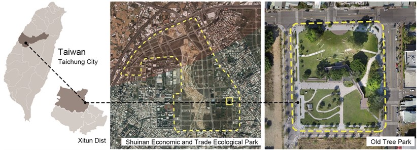
Recently, the population of Taichung City has been growing rapidly due to the gradual implementation of many major municipal construction projects and high economic activity. Most of the immigrant population is concentrated in the metropolitan area, and the population of the Beitun District has increased the most rapidly. This area was originally the Shuinan Airport, which was established in 1911 and relocated in 2004. The area was built into a new feature of Taichung City, the Taichung Shuinan Economic and Trade Ecological Park. The park, which is the focus of this study, called Old Tree Park, was established in a metropolitan area of about 1.27 hectares in 2011. Old Tree Park retained the original historical landscape and was designed with humanistic conservation, ecological sustainability, and environmental symbiosis as the main axes of design. It has a variety of environmental spaces and great historical value. Old Tree Park is bordered on all four sides by roadways. The base area is 170 meters, and it is situated 300 meters from the main arterial road, as shown in Fig. 1.
Fig. 1The schematic of the test park
The scope of this study extended outward 100 meters from the edge of the base, as shown in Fig. 2. The land uses of this park and its surrounding areas are parkland, a residential area, an innovation and research and development special area, a cultural and educational area, and institutional land. Topographic changes, building heights and surrounding land use within the scope of the study affect the environmental parameters of this urban park. These parameters were used as the basis for the placement of instruments in the experimental field.
Fig. 2The scope of this study. (Bing Map)

2.2. Experimental erection and equipment description
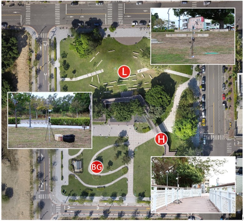
In this study, the measurement points were selected according to the geomorphological changes in the park. At the high position (H), horizontal grassland (BG) and low position (L) of this park, the environmental characteristics were measured. The measured data included atmospheric temperature, humidity, surface temperature, fine suspended particles, solar radiation value, wind speed, and wind direction. The Xitun measuring station of the Taichung Meteorological Bureau was used as a control group for the environmental background to monitor micro-climate changes with different geomorphology, as shown in Fig. 3.
Fig. 3The distribution schematic of the measurement points
3. Methodology
3.1. Environmental modelling
The terrain and topographic measurements in this study were conducted using a quadcopter unmanned aerial vehicle (UAV) for aerial surveys of the experimental site. The 3DR Solo drone equipped with a GOPRO Hero 4 camera was employed for capturing images in various angles, including nadir (90°), oblique (60°), and low-oblique (30°), to enhance the accuracy of the model. The collected images were processed using Pix4Dmapper software for model generation. The flight pitch angle and other detailed data are crucial for subsequent processing, analysis, and computation of the images, as they directly impact the accuracy of the 3D modeling [35].
Fig. 4UAV environmental modeling analysis diagram
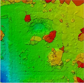
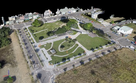
Based on the environmental model established through UAV terrain measurements, shown in Fig. 4, we can initially understand the park’s topography. The southern side of the park features steep slopes and dense tall trees, making it the highest area. The northern side is characterized by a lower elevation and serves as the park’s performance space. The western side consists of flat terrain with grass and planned walking paths. The measured on-site wind speed and direction, shown in Fig. 5, reveal that during the spring season, the prevailing winds are from the north and northwest. In the summer, southeast and southwest winds dominate, while the winter season is influenced by north winds. Based on these measurements, we can preliminarily infer that during the summer, the southeast winds may be obstructed by the resistance from the southern slopes and tall vegetation, resulting in reduced airflow. The lower elevation on the northern side may slow down the wind speed from the north and potentially increase the chance of suspended particulate matter deposition, enhancing the dust-trapping effect of the green space. The western side with its gentle slopes allows for smoother airflow.
Fig. 5The wind rose chart of the low position in spring, summer, and winter
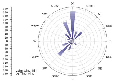
a) Spring
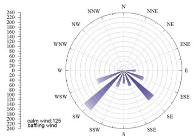
b) Summer
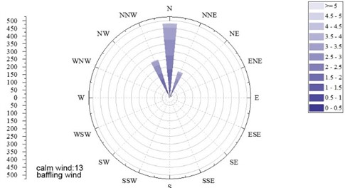
c) Winter
3.2. EM50 environmental measuring station
The measurement of environmental values in this study was conducted through an integrated monitoring station approach. The EM50 environmental measuring station, which included a data logger (EM50), temperature sensor (VP-4), solar radiation sensor (PYR Solar Radiation), surface temperature sensor (RT-1), and wind speed and direction sensor (Davis Cup) for hourly monitoring, is shown in Fig. 6(a). The measurement of soil infiltration status was carried out by setting up a two-meter-deep hole, drilled into the grassland to detect soil moisture content using a soil seepage meter, shown in Fig. 6(b).
Fig. 6Test instruments of this study
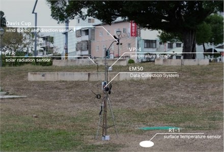
a) EM50 environmental station
b) Soil seepage meter
3.3. The measurement of airborne particulate matter
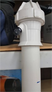
In this study, the Pantō PMS3003 Air Dust Sensor was used to detect atmospheric particulate matter. The PMS3003 is a digital universal particle concentration sensor that can be used to acquire the number of particles suspended in the air and output the result to a digital interface as a concentration. This device can record data on PM1.0, PM2.5 and PM10 suspended particles. The device includes an Arduino Uno (development version), PMS3003 (air dust sensor), XD-204 Data Logging shield (data logger, including SD card read and write module and RTC clock module), as shown in Fig. 7.
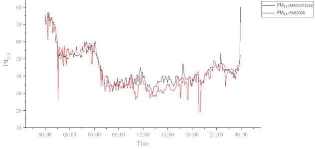
The PMS3003 suspension particle sensor is a low-cost experimental sensor. To test and verify the accuracy of this device, the test results were compared numerically with the highly accurate AEROCET 531S portable dust meter. The corrected PM2.5 value R2 of PMS3003 reached 0.842, a higher performance result, as shown in Fig. 8.
Fig. 7The developed Aerosol sensor
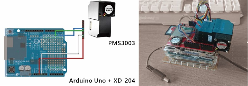
Fig. 8The comparison of the time history of the developed device and the AEROCET 531S portable dust meter
3.4. The correlation analysis for environmental factors
In this study, the time-history data of each measured environmental factor for each season were analyzed to assess the impact on the environmental correlations of heat environmental factors. Then Pearson correlation coefficient analysis was applied to find the correlations between each environmental factor. The Pearson correlation coefficient was used for analyzing the relationships between each environmental factor, which were expressed as as follows:
This method is used to investigate the linear correlation between two continuous variables . If the correlation coefficient between two variables is larger in absolute value, it means that the degree of mutual co-variation is greater. In general, if there is a positive correlation between two variables, then when increases, so does . Conversely, if there is a negative correlation between the two variables, then when increases, decreases. A value of 0 indicates that these two variables have no correlation. When is closer to +1 or –1, a higher linear correlation, Pearson’s correlation coefficient is calculated as follows:
where represents the th value of ; represents the th value of ; is the mean of variables; is the mean of variables.
The value can be regarded as the correlation effect and therefore can describe the strength of the association between two factors. Evans (J. D. Evans, 1996) defined the following five intensity grades: ± 0 to ± 0.19: very low; ± 0.20 to ± 0.39: low; ± 0.40 to ± 0.59: medium; ± 0.60 to ± 0.79: high; ± 0.8 to ± 1.0: very high. The correlation coefficients are explained in Table 1 as follows:
Table 1The degrees of correlation of the values of Pearson’s correlations
Pearson’s | ± 0 to ± 0.19 | ± 0.20 to ± 0.39 | ± 0.40 to ± 0.59 | ± 0.60 to ± 0.79 | ± 0.8 to ± 1.0 |
Degree of correlation | Very low | Low | Medium | High | Very high |
3.5. Three-dimensional scatter plot
To investigate the correlations among the surface temperatures of the structures, the atmospheric temperature and solar radiation values, and among the PM2.5 and PM10 concentrations of the suspended particles and the atmospheric temperature and wind speed, a three-dimensional scatter plot was used to explore the correlations among the variables. The relationships among the continuous independent variable and the other two continuous corresponding variables thus represented the relationships among the three continuous independent variables for investigation of the correlations among important factors.
4. Test results and discussions
The test of this research was a one-year long-term experiment. Because the climate characteristics of spring and autumn are similar, this study examined data from three representative days of weather for each season.
4.1. The surface temperature of landscape elements and airborne particles
4.1.1. The surface temperature of landscape elements
The surface temperatures of the landscape elements in the park in the spring, summer and winter are shown in Figs. 9-11.
Fig. 9The surface temperatures of landscape elements in the park in spring
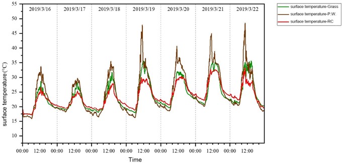
Fig. 10The surface temperatures of landscape elements in the park in summer
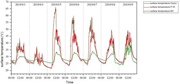
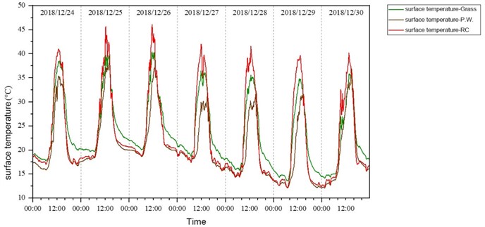
Fig. 9 shows that the most drastic changes in surface temperature in spring were those of wood-plastic composites, followed by dried grass, while that of concrete was the lowest. The maximum temperature of wood-plastic composites was 48.5 °C, that of grass was 35.2 °C, and that of concrete was 33.1 °C. In summer, the surface temperature of the wood-plastic composites still varied the most, followed by that of concrete, while that of grassland changed smoothly. The maximum temperature of the wood-plastic composites was 61.1 °C, that of concrete was 49.8 °C, and that of grass was 33 °C, as shown in Fig. 10. The surface temperature of the grassland was most greatly affected by the soil moisture content. In the early stage of continuous monitoring, the soil water content was between 0.15 % and 0.18 %, and the surface temperature of the grassland changed smoothly. However, when the soil moisture content was less than 0.12 %, the surface temperature of the grassland reached 45 °C. In winter, the surface temperature of concrete was the highest, followed by that of grassland, and the lowest was that of wood–plastic composites. The maximum surface temperature of the concrete structure was 46 °C, that of the grass was 40.3 °C, and that of the wood-plastic composites was 34.3 °C, as shown in Fig. 11.
Fig. 11The surface temperatures of landscape elements in the park in winter
4.1.2. Airborne particles
Time histories of the variation in PM2.5 and PM10 concentrations in the park in spring, summer and winter are shown in Figs. 12-15.
Fig. 12Time history of variations in PM2.5 and PM10 concentrations in spring
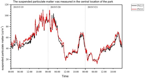
The suspended particulate matter was measured in the central location of the park, as shown in Fig. 12. According to the time histories of variations in suspended particulate matter, the maximum concentrations of suspended PM2.5 and PM10 appeared at about 8:00 PM. The maximum concentration of PM2.5 was 111 μg/m3, and the maximum concentration of PM10 was 125 μg/m3. The time histories of variations in PM2.5 and PM10 in summer are shown in Fig. 13 and 14. Air quality in summer was affected by atmospheric temperature, relative humidity and wind speed. Therefore, the changes in PM2.5 and PM10 concentrations at the high (H), horizontal grass (BG) and low (L) positions of the park were selected for discussion.
Fig. 13Time history of variations in PM2.5 concentrations in summer
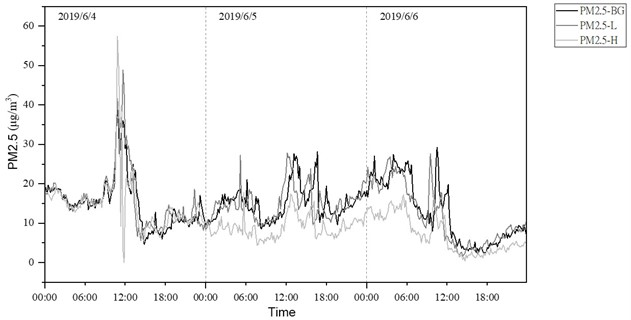
Fig. 14Time history of variations in PM10 concentrations in summer
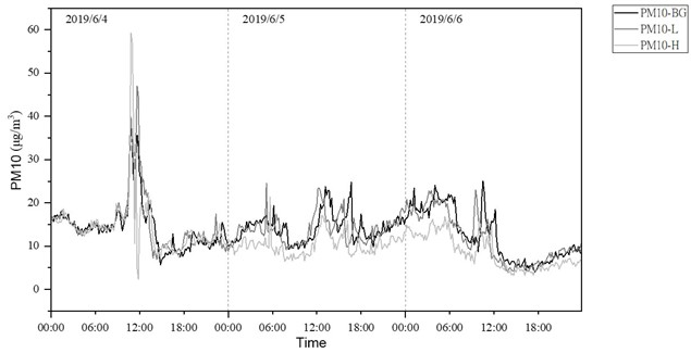
Fig. 15Time history of variations in PM2.5 and PM10 concentrations in winter
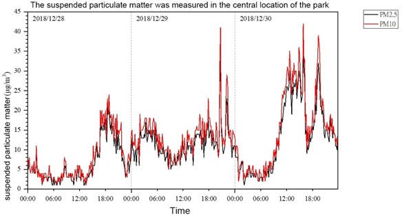
Fig. 14 and 15 show that the maximum concentrations of PM2.5 were 57.4 μg/m3 at the high position and 41.6 μg/m3 at the low position. At the grass position, it was 39.2 μg/m3. At the same time, the maximum PM10 concentrations were 77.2 μg/m3 at the high position, 50.8 μg/m3 at the low position, and 48.8 μg/m3 at the grass position. At other times, the variations in the trend of PM2.5 concentrations at the low position were consistent with those of the grass position. However, the PM2.5 concentrations at the high position were lower than those at the other two stations. In addition, Fig. 14 and 15 show that the low and grass positions exceeded the air quality standard mostly in the early morning, and the relative humidity was higher than that of the high position. In winter, as shown in Fig. 15, the maximum PM2.5 and PM10 concentrations, i.e., 35 and 42 μg/m3, appeared at 4:00 PM. The trend in the variation of air quality showed that in winter, the air quality in this park was lowest each day from 5:00 PM to 10:00 PM.
4.2. Correlation analysis of various factors of landscape elements in the park
The major factors affecting the surface temperature of the landscape elements in the park were atmospheric temperature, relative humidity, solar radiation value and wind speed. Therefore, Pearson’s correlation analysis was applied to analyze the correlations between factors. The results for spring, summer and winter are listed in Tables 2, 3 and 4, respectively. The correlations between the factors are described as follows.
Table 2Correlation analysis results of each factor – Spring
Correlation analysis | Atmospheric temperature | Relative humidity | Solar radiation | Wind speed | Grass Temp. | Concrete Temp. | Wood-plastic composite Temp. | |
Atmospheric temperature | Pearson’s | 1 | –.939** | .731** | .788** | .928** | .964** | .866** |
Sig.(Two Tailed) | 0.000 | 0.000 | 0.000 | 0.000 | 0.000 | 0.000 | ||
Relative humidity | Pearson’s | –.939** | 1 | –.818** | –.692** | –.949** | –.931** | –.894** |
Sig.(Two Tailed) | 0.000 | 0.000 | 0.000 | 0.000 | 0.000 | 0.000 | ||
Solar radiation | Pearson’s | .731** | –.818** | 1 | .625** | .917** | .817** | .881** |
Sig.(Two Tailed) | 0.000 | 0.000 | 0.000 | 0.000 | 0.000 | 0.000 | ||
Wind speed | Pearson’s | .788** | –.692** | .625** | 1 | .746** | .819** | .713** |
Sig.(Two Tailed) | 0.000 | 0.000 | 0.000 | 0.000 | 0.000 | 0.000 | ||
Grass | Pearson’s | .928** | –.949** | .917** | .746** | 1 | .956** | .950** |
Sig.(Two Tailed) | 0.000 | 0.000 | 0.000 | 0.000 | 0.000 | 0.000 | ||
Concrete | Pearson’s | .964** | –.931** | .817** | .819** | .956** | 1 | .939** |
Sig.(Two Tailed) | 0.000 | 0.000 | 0.000 | 0.000 | 0.000 | 0.000 | ||
Wood-plastic composite | Pearson’s | .866** | –.894** | .881** | .713** | .950** | .939** | 1 |
Sig.(Two Tailed) | 0.000 | 0.000 | 0.000 | 0.000 | 0.000 | 0.000 | ||
**0.01 level (Two Tailed), significant correlation | ||||||||
Table 3Correlation analysis results of each factor – Summer
Correlation analysis | Atmospheric temperature | Relative humidity | Solar radiation | Wind speed | Grass Temp. | Concrete Temp. | Wood-plastic composite Temp. | |
Atmospheric temperature | Pearson’s | 1 | –.916** | .788** | .738** | .855** | .884** | .878** |
Sig.(Two Tailed) | 0.000 | 0.000 | 0.000 | 0.000 | 0.000 | 0.000 | ||
Relative humidity | Pearson’s | –.916** | 1 | –.609** | –.577** | –.723** | –.725** | –.774** |
Sig.(Two Tailed) | 0.000 | 0.000 | 0.000 | 0.000 | 0.000 | 0.000 | ||
Solar radiation | Pearson’s | .788** | –.609** | 1 | .721** | .600** | .742** | .905** |
Sig.(Two Tailed) | 0.000 | 0.000 | 0.000 | 0.000 | 0.000 | 0.000 | ||
Wind speed | Pearson’s | .738** | –.577** | .721** | 1 | .736** | .806** | .658** |
Sig.(Two Tailed) | 0.000 | 0.000 | 0.000 | 0.000 | 0.000 | 0.000 | ||
Grass temp. | Pearson’s | .855** | –.723** | .600** | .736** | 1 | .946** | .649** |
Sig.(Two Tailed) | 0.000 | 0.000 | 0.000 | 0.000 | 0.000 | 0.000 | ||
Concrete Temp. | Pearson’s | .884** | –.725** | .742** | .806** | .946** | 1 | .762** |
Sig.(Two Tailed) | 0.000 | 0.000 | 0.000 | 0.000 | 0.000 | 0.000 | ||
Wood-plastic composite Temp | Pearson’s | .878** | –.774** | .905** | .658** | .649** | .762** | 1 |
Sig.(Two Tailed) | 0.000 | 0.000 | 0.000 | 0.000 | 0.000 | 0.000 | ||
**.0.01 level (Two Tailed), significant correlation | ||||||||
Table 4Correlation analysis results of each factor – Winter
Correlation analysis | Atmospheric temperature | Relative humidity | Solar radiation | Wind speed | Grass Temp. | Concrete Temp. | Wood-plastic composite Temp. | |
Atmospheric temperature | Pearson’s | 1 | –.869** | .758** | .013 | .945** | .888** | .954** |
Sig.(Two Tailed) | .000 | .000 | .795 | .000 | .000 | .000 | ||
Relative humidity | Pearson’s | –.869** | 1 | –.846** | –.145** | –.930** | –.899** | –.908** |
Sig.(Two Tailed) | .000 | .000 | .003 | .000 | .000 | .000 | ||
Solar radiation | Pearson’s | .758** | –.846** | 1 | .215** | .898** | .964** | .792** |
Sig.(Two Tailed) | .000 | .000 | .000 | .000 | .000 | .000 | ||
Wind speed | Pearson’s | .013 | –.145** | .215** | 1 | .133** | .132** | .014 |
Sig.(Two Tailed) | .795 | .003 | .000 | .006 | .006 | .767 | ||
Grass Temp. | Pearson’s | .945** | –.930** | .898** | .133** | 1 | .973** | .954** |
Sig.(Two Tailed) | .000 | .000 | .000 | .006 | .000 | .000 | ||
Concrete Temp. | Pearson’s | .888** | –.899** | .964** | .132** | .973** | 1 | .909** |
Sig.(Two Tailed) | .000 | .000 | .000 | .006 | .000 | .000 | ||
Wood-plastic composite Temp. | Pearson’s | .954** | –.908** | .792** | .014 | .954** | .909** | 1 |
Sig.(Two Tailed) | .000 | .000 | .000 | .767 | .000 | .000 | ||
**. 0.01 level (Two Tailed), significant correlation | ||||||||
4.3. Influence of atmospheric temperature and wind speed on the surface temperature of the landscape elements in the park
The correlation analysis results in Table 2 show that the strongest effects of atmospheric temperature on the surface temperature of the landscape elements were those of concrete, grass and wood–plastic composite, Pearson’s .964**, .928** and .866**, respectively. The correlation analysis results for summer, listed in Table 3, show that the strongest effects of atmospheric temperature on the surface temperature of the landscape elements were those of concrete, wood–plastic composite and grass, Pearson’s .884**, 878** and .855**, respectively. The analysis results in winter, listed in Table 4, show that the greatest effects of atmospheric temperature on the surface temperature of the landscape elements were those of wood-plastic composite, grass and concrete, Pearson’s .954**, .945** and .888** respectively. The correlations between atmospheric temperature and the surface temperatures of the landscape elements in the park were extremely high in each season. Regardless of the season, the surface temperature of each landscape element rose under the influence of atmospheric temperature. In spring and summer, atmospheric temperature had the most significant influence on the temperature of concrete, and in winter, on the temperature of wood-plastic composite.
The correlations of wind speed in spring and summer with the surface temperature of concrete were .819** and .806**, respectively. In spring, the correlations between wind speed and the surface temperatures of grass and wood-plastic composite structures were high, respectively .746** and .713**. In summer, the correlations between wind speed and the surface temperatures of grassland and wood-plastic composite were also high, .736** and .658**, respectively. In winter, the correlations of wind speed with the surface temperatures of landscape elements in the park were very low, .133** for grassland, .0.132** for concrete and .014** for wood-plastic composite.
4.3.1. Effect of relative humidity on the surface temperature of the landscape elements
The effects of relative humidity on the surface temperatures of the landscape elements in spring were highly negatively correlated. The correlations with grass, concrete and wood-plastic composite was respectively –.949**, –.931** and –.894**. In summer, the correlations were also very high and negative. For wood–plastic composite, concrete and grass, they were –.774**, –.725** and –.723** respectively. In winter, the correlation values of the grass, wood–plastic composite and concrete were extremely negative: –.930**, –.908** and –.899**, respectively. The analysis results showed that the surface temperature of grassland was most significantly negatively correlated with the influence of relative humidity in spring and winter. In summer, the negative correlation between relative humidity and wood-plastic composite was the most significant.
4.3.2. Effect of solar radiation on surface temperatures of the landscape elements
The correlation analysis results of the solar radiation effect on the surface temperature of the landscape elements in spring showed that the Pearson’s value of grass was .917**, the highest impact, followed by wood-plastic composite ( .881**) and concrete ( .817**), all of which were extremely high positive correlations. In summer, the correlation between solar radiation and wood–plastic composite (Pearson’s .905**) was extremely high and positive, while those for concrete and grassland were high, .742** and .600**, respectively. In winter, the correlations between solar radiation and concrete (Pearson's .964**) and grassland ((Pearson’s .898**) were extremely high. The correlation with wood-plastic composite was also high, .792**. The effects of solar radiation on the surface temperatures of grassland and wood-plastic composite in spring and summer were the most significant, respectively. In winter, the surface temperature of concrete was the one which was most strongly affected by solar radiation.
4.3.3. Analysis results of three-dimensional scatterplot
The sampled scattering in the upper part of the scatter plot was mainly affected by the high temperature and high thermal radiation values. The bottom refers to the area of low temperature and low radiation value, and the surface temperature of the structure is relatively low. The analysis results of three-dimensional scatter plots with the surface temperatures of three various landscape elements in three different seasons are shown in Figs. 16-18.
Fig. 16Three-dimensional scatterplot showing the land surface temperature correlation analysis for atmospheric temperature and solar radiation in spring
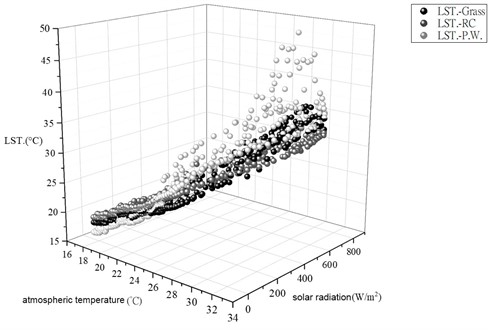
Fig. 17Three-dimensional scatterplot showing the land surface temperature correlation analysis for atmospheric temperature and solar radiation in summer
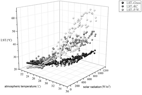
Fig. 18Three-dimensional scatterplot showing the land surface temperature correlation analysis for atmospheric temperature and solar radiation in winter
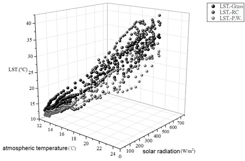
The three-dimensional scatter plot of three different surface temperatures of LST in Fig. 16 shows that, for the surface temperatures of three different landscape elements in spring, the atmospheric temperature and thermal radiation values had a positive trend. The three-dimensional scatter plot in Fig. 16 is inclined towards the area of high temperature and high thermal radiation values. Especially, the surface temperature of wood–plastic composite was greatly affected by higher solar radiation and high atmospheric temperature. The higher solar radiation and higher atmospheric temperature had a large impact on the surface temperatures of concrete and grassland with the same trend.
Fig. 17 presents a three-dimensional scatter plot for summer, which shows a positive trend in the surface temperatures of wood-plastic composite and concrete with the atmospheric temperature and thermal radiation. The three-dimensional scatter plot is inclined towards the area of high temperature and high thermal radiation. The surface temperature of wood-plastic composite was greatly affected by solar radiation and atmospheric temperature. The atmospheric temperature and thermal radiation values had a significant impact on the surface temperature of concrete. In contrast, the surface temperature of grassland had a relatively gentle change, indicating that the grassland temperature had a good temperature regulation effect in summer.
Fig. 18 is a three-dimensional scatter plot for winter, revealing that, for the surface temperatures of these three landscape elements, the atmospheric temperature and the thermal radiation value had a positive trend. The three-dimensional scatter plot is inclined towards the area of high temperature and high thermal radiation, and atmospheric temperature and thermal radiation values had significant impacts on the surface temperatures of grassland and concrete.
4.4. Correlation analysis of airborne particles with various factors
The results of the correlation analysis between the various factors and the concentrations of suspended particles in the three different seasons of the park are shown in Tables 5, 6, and 7. The factors affecting the concentrations of suspended particles were explored by Pearson correlation analysis based on the measured data for each season. It can be seen from these tables that the main factors affecting the concentrations of suspended particles were wind speed, atmospheric temperature and relative humidity, and the correlations between the various factors in each season are explained as follows.
4.4.1. Effect of wind speed on concentrations of suspended particles
As shown in Table 5, correlations between wind speed and the concentrations of PM2.5 and PM10 suspended particles in spring were –. 431** and –. 427** respectively, indicating medium negative correlations. The residual concentration of suspended particles and wind speed had a negative correlation change.
Table 5The correlation analysis between PM2.5 and PM10 concentrations and various environmental factors in spring
Correlation Analysis | Atmospheric Temp. | Relative humidity | Solar radiation | Wind speed | PM2.5 | PM10 | |
Atmospheric Temp, | Pearson’s | 1 | –.939** | .731** | .788** | –.291** | –.280** |
Sig. (two tailed) | 0.000 | 0.000 | 0.000 | 0.000 | 0.000 | ||
Relative huminity | Pearson’s r | –.939** | 1 | –.818** | –.692** | .213** | .193** |
Sig. (two tailed) | 0.000 | 0.000 | 0.000 | 0.000 | 0.000 | ||
Solar radiation | Pearson’s r | .731** | –.818** | 1 | .625** | –.289** | –.269** |
Sig. (two tailed) | 0.000 | 0.000 | 0.000 | 0.000 | 0.000 | ||
Wind speed | Pearson’s r | .788** | –.692** | .625** | 1 | –.431** | –.427** |
Sig. (two tailed) | 0.000 | 0.000 | 0.000 | 0.000 | 0.000 | ||
PM2.5 | Pearson’s r | –.291** | .213** | –.289** | –.431** | 1 | .990** |
Sig. (two tailed) | 0.000 | 0.000 | 0.000 | 0.000 | 0.000 | ||
PM10 | Pearson’s r | –.280** | .193** | –.269** | –.427** | .990** | 1 |
Sig. (two tailed) | 0.000 | 0.000 | 0.000 | 0.000 | 0.000 | ||
**. level (Two Tailed), significant correlation | |||||||
Table 6The correlation analysis between PM2.5 and PM10 concentrations and various environmental factors in summer
Correlation Analysis | Atmospheric Temp. | Relative humidity | Solar radiation | Wind speed | PM2.5 | PM10 | |
Atmospheric Temp, | Pearson’s | 1 | –.916** | .788** | .738** | –.186** | –.204** |
Sig.(two tailed) | 0.000 | 0.000 | 0.000 | 0.000 | 0.000 | ||
Relative humidity | Pearson’s | –.916** | 1 | –.609** | –.577** | .316** | .337** |
Sig.(two tailed) | 0.000 | 0.000 | 0.000 | 0.000 | 0.000 | ||
Solar radiation | Pearson’s | .788** | –.609** | 1 | .721** | –0.068 | –0.083 |
Sig.(two tailed) | 0.000 | 0.000 | 0.000 | 0.157 | 0.086 | ||
Wind speed | Pearson’s | .738** | –.577** | .721** | 1 | –.111* | –.106* |
Sig.(two tailed) | 0.000 | 0.000 | 0.000 | 0.020 | 0.028 | ||
PM2.5 | Pearson’s | –.186** | .316** | -0.068 | –.111* | 1 | .992** |
Sig.(two tailed) | 0.000 | 0.000 | 0.157 | 0.020 | 0.000 | ||
PM10 | Pearson’s | –.204** | .337** | -0.083 | –.106* | .992** | 1 |
Sig.(two tailed) | 0.000 | 0.000 | 0.086 | 0.028 | 0.000 | ||
**. level (Two Tailed), significant correlation | |||||||
Table 6 shows that the correlation coefficients of wind speed and PM2.5 and PM10 in summer were –.111** and –.106**, respectively, indicating very low negative correlation. In Table 7, the correlations of winter wind speed and concentrations of PM2.5 and PM10 were –. 416** and –. 408**, respectively, indicating moderate negative correlations, and the stagnation of suspended particle concentrations was negatively correlated with wind speed.
From these results, the stagnation of the suspended particle concentrations in spring and winter was moderately negatively correlated with wind speed. In summer, the retention of suspended particle concentrations and wind speed showed a negative correlation change, and the impact was not significant.
Table 7The correlation analysis between PM2.5 and PM10 concentrations and various environmental factors in winter
Correlation Analysis | Atmospheric Temp. | Relative humidity | Solar radiation | Wind Speed | PM2.5 | PM10 | |
Atmospheric Temp | Pearson’s | 1 | –.869** | .758** | .013 | .292** | .270** |
Sig.(two tailed) | .000 | .000 | .795 | .000 | .000 | ||
Relative humidity | Pearson’s | –.869** | 1 | –.846** | –.145** | –.249** | –.234** |
Sig.(two tailed) | .000 | .000 | .003 | .000 | .000 | ||
Solar radiation | Pearson’s | .758** | –.846** | 1 | .215** | .014 | .000 |
Sig.(two tailed) | .000 | .000 | .000 | .771 | .993 | ||
Wind speed | Pearson’s | .013 | –.145** | .215** | 1 | –.416** | –.408** |
Sig.(two tailed) | .795 | .003 | .000 | .000 | .000 | ||
PM2.5 | Pearson’s | .292** | –.249** | .014 | –.416** | 1 | .983** |
Sig.(two tailed) | .000 | .000 | .771 | .000 | .000 | ||
PM10 | Pearson’s | .270** | –.234** | .000 | –.408** | .983** | 1 |
Sig.(two tailed) | .000 | .000 | .993 | .000 | .000 | ||
**. level (Two Tailed), significant correlation | |||||||
4.4.2. Effect of relative humidity on concentrations of suspended particulates
As shown in Table 5, the correlation analysis results for relative humidity and suspended PM2.5 and PM10 concentrations were .213** and .193** respectively, indicating a low correlation for PM2.5 and a very low one for PM10. The correlations of PM2.5 and PM10 concentrations in summer were Pearson's .316** and .337**, respectively, which were low positive correlations. As shown in Table 7, in winter, the correlations for the PM2.5 and PM10 concentrations were low and negative, –.249** and –. 234**.
The results showed that the effect of relative humidity on the concentrations of suspended particles was not significant.
4.4.3. Effects of atmospheric temperature and solar radiation on the concentration of suspended particles
The correlation analysis results in Table 5 showed that atmospheric temperature and solar radiation had low correlations with the concentrations of suspended PM2.5 and PM10 particles, –.291** and Pearson’s –.280** for atmospheric temperature and –.289** and Pearson’s –.269** for solar radiation, indicating low negative correlations with these two factors in spring.
Table 6 shows that the correlations between PM2.5 and PM10 concentrations and atmospheric temperature in summer were –.186** and Pearson’s –.204** respectively, indicating a very low negative correlation for PM2.5 concentration and low negative correlation for PM10 concentration in summer. The correlations of solar radiation with the concentrations of suspended particles were very low for PM2.5 and PM10, –.068** and –.083** respectively.
The results for winter in Table 7 revealed that the correlations of atmospheric temperature with concentrations of suspended PM2.5 and PM10 particles were .292** and .270** respectively, showing a low positive correlation. The correlations of solar radiation with concentrations of suspended PM2.5 and PM10 particles were .014** and Pearson’s .000** respectively, indicating very low positive correlations.
The results of the analysis showed that the effects of atmospheric temperature and solar radiation on the concentrations of suspended particles were not significant in spring, summer, or winter.
4.4.4. Correlation analysis results of three-dimensional scatterplot
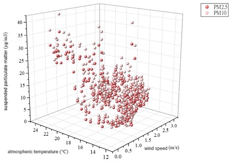
The results of three-dimensional scatter correlation analysis of PM2.5 and PM10 concentrations are shown in Fig. 19, 20 and 21 for spring, summer and winter, respectively. Tables 5 and 7 reveal that the PM2.5 and PM10 concentrations in spring and winter were mainly related to atmospheric temperature and wind speed. Therefore, Fig. 19 and 21 show three-dimensional scatter plots of PM2.5 and PM10 concentrations with atmospheric temperature and wind speed. Table 6 shows that PM2.5 and PM10 concentrations in summer were mainly related to atmospheric temperature and relative humidity. Fig. 20 shows a three-dimensional scatter plot of PM2.5 and PM10 concentrations with atmospheric temperature and relative humidity.
Fig. 19Correlation analysis between PM2.5 and PM10 concentrations and atmospheric temperature and wind speed in spring
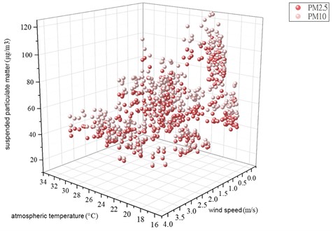
Fig. 20Correlation analysis between PM2.5 and PM10 concentrations and atmospheric temperature and relative humidity in summer
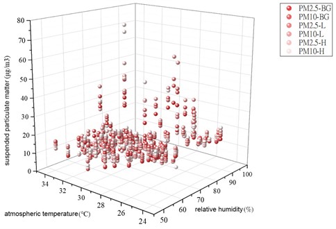
Fig. 19 shows that the sampled scatter points in spring were mainly concentrated at low wind speeds and low temperatures, and PM2.5 and PM10 concentrations were high. In areas with high wind speeds and high temperatures, the PM2.5 and PM10 concentrations were relatively low. The three-dimensional scatter plot tilts towards the area with low wind speed and low temperature, indicating the influence of wind speed and atmospheric temperature on PM2.5 and PM10 concentrations.
Fig. 20 shows that the sampled scattering points in summer were mainly concentrated in atmospheric temperatures of 28-35 °C and relative humidity of 60-90 %. The PM2.5 and PM10 concentrations were low. When the atmospheric temperature was 26-32 °C and the relative humidity was higher than 90 %, the PM2.5 and PM10 concentrations were high. In areas with high wind speeds and high atmospheric temperatures, the concentration of suspended particles was relatively low. The three-dimensional scatter plot tilts towards the area with low wind speed and low atmospheric temperature, demonstrating the influence of wind speed and atmospheric temperature on the PM2.5 and PM10 concentrations. It can be found that high atmospheric temperature and high relative humidity before and after rainfall will cause the PM2.5 and PM10 concentrations to rise and remain.
Fig. 21 reveals that the sampled scatter points in winter were mainly concentrated at the bottom of high wind speed and low atmospheric temperature. The bottom refers to areas with high wind speeds and low atmospheric temperatures, and PM2.5 and PM10 concentrations were relatively low. The three-dimensional scatterplot tilts towards the area with low wind speed and high atmospheric temperature, indicating the influence of wind speed and atmospheric temperature on PM2.5 and PM10 concentrations.
Fig. 21Correlation analysis between PM2.5 and PM10 concentrations and atmospheric temperature and wind speed in winter
4.4.5. Analysis of the relationship between airborne particles and wind speed
The results of the analysis revealed that atmospheric particulate matter concentrations are greatly affected by the monsoon in spring and winter. In summer, they are less affected by the monsoon because of the direction of the wind. Therefore, this study compared the changes in airborne particles in the park with data from the adjacent Xitun Station of the Central Weather Bureau to explore the changes in air quality in the park. The results are shown in Fig. 22 and 23, which compare the variations in PM2.5 and PM10 concentrations and wind speed of the test park with the relevant data of Xitun Station in spring. Figures 24 and 25 show the time histories of variations in PM2.5 and PM10 concentrations in summer. Fig. 26 and 27 compare the results of those data in winter.
Figs. 22 and 23 show that PM2.5 and PM10 concentrations are related to wind speed. When the wind speed in the park was lower than that of the weather measurement station, the PM2.5 concentrations in the park were higher than those at the weather measurement station. Nevertheless, the variations in PM10 concentrations were the opposite. PM2.5 and PM10 concentrations began to increase at 6:00 AM and to decrease at 6:00 PM. The highest PM2.5 concentrations appeared around 8:40 PM, reaching a maximum of 96 ug/m3, and the highest PM10 concentration was at about 125 ug/m3 at 1:00 PM. The reduction of suspended particles was less significant in the park.
Fig. 22PM2.5 and wind speed comparison between Park and Xitun Measurement Station in spring
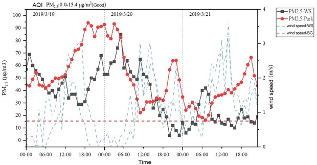
Fig. 23PM10 and wind speed comparison between the park and the Xitun Measurement Station in spring
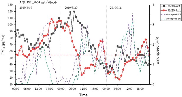
Fig. 24Time history of variations in PM2.5 concentration at the park in summer
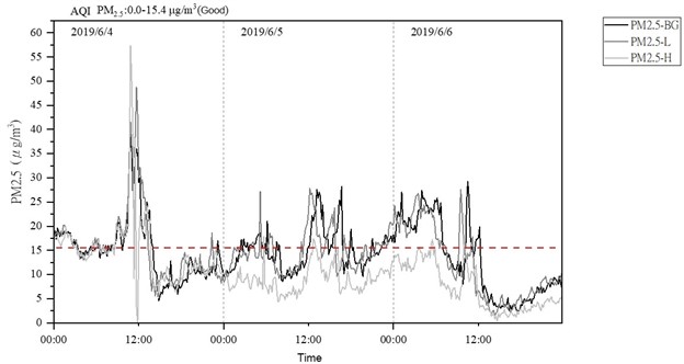
Figs. 24 and 25 reveal that PM2.5 and PM10 concentrations were most greatly affected by wind speed and rainfall at the low measurement point (L) in summer, when they were as high as 60.8 ug/m3 and 78 ug/m3 respectively. The periods of fine air quality suitable for users were around 07:00–10:00 AM and after 5:00 PM.
Fig. 25Time history of variations in PM10 concentration at the park in summer
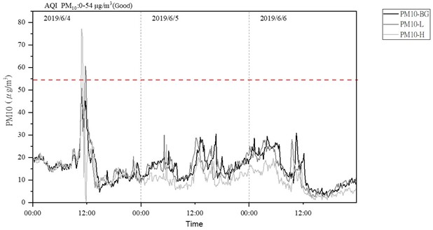
Fig. 26Comparison of PM2.5 concentration and wind speed between the park and the Xitun Measurement Station in winter
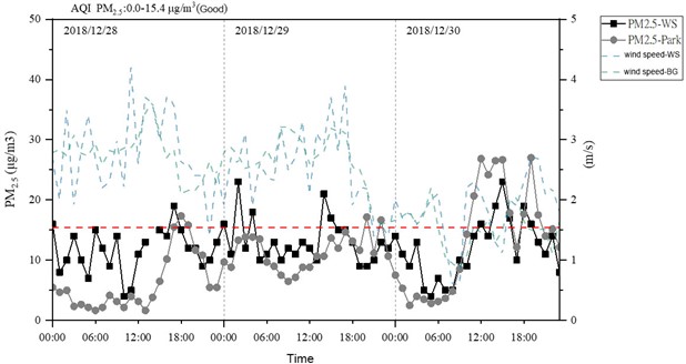
Fig. 27Comparison of PM10 concentration and wind speed between the park and the Xitun Measurement Station in winter
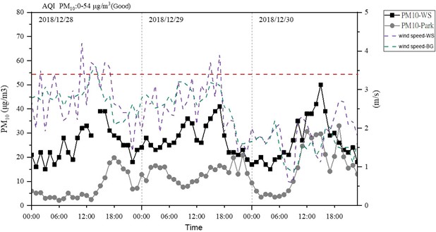
Figs. 26 and 27 show the relation of PM2.5 and PM10 concentrations to the monsoon of winter. When the monsoon wind was strong, PM2.5 and PM10 concentrations in the park were below those at the weather measurement station. The highest PM2.5 concentration appeared at 03:00 PM, reaching a maximum of 27 ug/m3, and the highest PM10 concentration was 33 ug/m3 at 07:00 PM. These measured data were compared with those of the Xitun measurement station, and it was found that the green space significantly reduced the concentrations of suspended particles in the park.
4.5. Correlations between seasonal wind directions and airborne particles
The results in Tables 5, 6 and 7 revealed that PM2.5 and PM10 concentrations have a moderate negative correlation with wind speed in the spring and winter seasons. They have extremely low negative correlations with wind speeds in summer. Figures 22, 23, 26 and 27 clearly show that the PM2.5 and PM10 concentrations decline at high wind speeds. However, the PM2.5 and PM10 concentrations are significantly higher in spring than in the other seasons.
5. Conclusions
In this study, the outdoor environmental factors in the test park were monitored for a long-term test period. The following conclusions are based on the cross-analysis of the relevant experimental data.
1) The measurement results indicate that atmospheric temperatures have the greatest influence on concrete surface temperatures in spring and summer, and then on wood-plastic composite in winter, followed by grasslands. Especially, the surface temperature of grassland with 10 % water content is higher than that of concrete. The main reason for exploring the temperature change of grassland is the influence of the thermal conductivity of the landscape elements, and the moisture content of the grassland soil should be maintained at 15-18 % for a specific cooling function to affect the environment.
2) The effects of wind speed on concrete surface temperatures in spring and summer had very high positive correlations, and in winter, very low positive correlations. Therefore, in the future, when an urban park is constructed, it is necessary to consider the direction of the urban wind field in the configuration of the various landscape elements of the park.
3) Relative humidity in this park had a very high negative correlation with the surface temperatures of the landscape elements. Higher relative humidity in spring and winter was correlated with lower grassland surface temperatures, and in summer, lower wood-plastic composite surface temperatures. It is recommended that a water spray device be installed on the hard pavement of the park to increase the relative humidity in summer and cool the environment.
4) Solar radiation had very high positive correlations with the surface temperatures of the landscape elements. Solar radiation had the greatest influence on the temperature of the grass in spring, but on the temperatures of both concrete and grass in summer. In winter, solar radiation influenced on the surface temperatures of the concrete and grass. It is recommended that shading devices or shade trees be installed to improve the environmental comfort related to changes in the rising and falling angles of the sun.
5) The three-dimensional scatter plots of surface temperatures (LST) showed that atmospheric temperature and solar radiation had significant impacts on the surface temperatures of landscape elements in spring and winter. The grassland had a good temperature regulation effect in summer and spring.
6) The analysis of factors influencing PM2.5 and PM10 concentrations showed that the air quality in spring and winter was affected by wind speeds, which were higher than those in summer, and relative humidity and atmospheric temperature had little effect on air quality.
7) The three-dimensional scatter plot of the PM2.5 and PM10 concentrations in spring and summer, when the climate changed towards high temperature and high relative humidity, led to increases in, and the retention of, suspended particle concentrations. In winter, when the winter wind speed is low and the atmospheric temperature is relatively high, the concentration of suspended particles can easily increase.
Suggestions:
1) Based on the findings of this study, the use of concrete and wood-plastic composite materials should be reduced, and building materials with low heat storage should be employed as much as possible to improve the environmental factors in existing parks. In addition, a certain level of moisture content should be maintained in grasslands so that the grassland can maintain growth, not become desiccated, and act as a heat storage material in winter.
2) The air quality in this park was negatively correlated with wind speed and correlated with atmospheric temperature in winter, but the air quality was related to high temperature and high humidity in summer. The wind rose charts revealed that the direction of the monsoon direction affected the air quality of the park very dramatically. Therefore, the influence of the monsoon must be considered in the design to introduce natural wind fields and thereby improve the air quality.
References
-
“Urban Heat Island.” National Geographic. https://www.nationalgeographic.org/encyclopedia/urban-heat-island/
-
C. O. ’Malley, P. A. E. Piroozfarb, E. R. P. Farr, and J. Gates, “An Investigation into minimizing urban Heat Island (UHI) effects: a UK perspective,” Energy Procedia, Vol. 62, pp. 72–80, 2014, https://doi.org/10.1016/j.egypro.2014.12.368
-
J. Martin-Vide, P. Sarricolea, and M. C. Moreno-Garcã A., “On the definition of urban heat island in tensity: the "rural" reference,” Frontiers in Earth Science, Vol. 3, Jun. 2015, https://doi.org/10.3389/feart.2015.00024
-
X. Yang, Y. Chen, L. L. H. Peng, and Q. Wang, “Quantitative methods for identifying meteorological conditions conducive to the development of urban heat islands,” Building and Environment, Vol. 178, p. 106953, Jul. 2020, https://doi.org/10.1016/j.buildenv.2020.106953
-
Huanchun Huang et al., “Influencing mechanisms of urban heat island on respiratory diseases,” Iranian Journal of Public Health, Vol. 48, No. 9, pp. 1636–1646, Sep. 2019.
-
J. A. Voogt and T. R. Oke, “Thermal remote sensing of urban climates,” Remote Sensing of Environment, Vol. 86, No. 3, pp. 370–384, Aug. 2003, https://doi.org/10.1016/s0034-4257(03)00079-8
-
S. W. Kim and R. D. Brown, “Urban heat island (UHI) intensity and magnitude estimations: A systematic literature review,” Science of The Total Environment, Vol. 779, p. 146389, Jul. 2021, https://doi.org/10.1016/j.scitotenv.2021.146389
-
M. Amani-Beni, B. Zhang, G.-D. Xie, and J. Xu, “Impact of urban park’s tree, grass and waterbody on microclimate in hot summer days: A case study of Olympic Park in Beijing, China,” Urban Forestry and Urban Greening, Vol. 32, pp. 1–6, May 2018, https://doi.org/10.1016/j.ufug.2018.03.016
-
Q. Xie and J. Li, “Detecting the cool island effect of urban parks in Wuhan: a city on rivers,” International Journal of Environmental Research and Public Health, Vol. 18, No. 1, p. 132, Dec. 2020, https://doi.org/10.3390/ijerph18010132
-
H. Algretawee, S. Rayburg, and M. Neave, “Estimating the effect of park proximity to the central of Melbourne city on Urban Heat Island (UHI) relative to land surface temperature (LST),” Ecological Engineering, Vol. 138, pp. 374–390, Nov. 2019, https://doi.org/10.1016/j.ecoleng.2019.07.034
-
Fukagawa K. and Aruninta A., “A study on the efficiency of designing urban park as cooling spot in the center of Bangkok – Targetting Raising Season,” EM International, Vol. 25, No. 2, pp. 537–541, 2019.
-
P. K. Cheung and C. Y. Jim, “Differential cooling effects of landscape parameters in humid-subtropical urban parks,” Landscape and Urban Planning, Vol. 192, p. 103651, Dec. 2019, https://doi.org/10.1016/j.landurbplan.2019.103651
-
F. Aram, E. Higueras García, E. Solgi, and S. Mansournia, “Urban green space cooling effect in cities,” Heliyon, Vol. 5, No. 4, p. e01339, Apr. 2019, https://doi.org/10.1016/j.heliyon.2019.e01339
-
W. Guo et al., “A study of subtropical park thermal comfort and its influential factors during summer,” Journal of Thermal Biology, Vol. 109, p. 103304, Oct. 2022, https://doi.org/10.1016/j.jtherbio.2022.103304
-
J. Zhang, Z. Gou, and Y. Lu, “Outdoor thermal environments and related planning factors for subtropical urban parks,” Indoor and Built Environment, Vol. 30, No. 3, pp. 363–374, Mar. 2021, https://doi.org/10.1177/1420326x19891462
-
H. Kong, N. Choi, and S. Park, “Thermal environment analysis of landscape parameters of an urban park in summer – A case study in Suwon, Republic of Korea,” Urban Forestry and Urban Greening, Vol. 65, p. 127377, Nov. 2021, https://doi.org/10.1016/j.ufug.2021.127377
-
S. Yilmaz, M. A. Irmak, and A. Qaid, “Assessing the effects of different urban landscapes and built environment patterns on thermal comfort and air pollution in Erzurum city, Turkey,” Building and Environment, Vol. 219, p. 109210, Jul. 2022, https://doi.org/10.1016/j.buildenv.2022.109210
-
M. Yuan, Y. Huang, H. Shen, and T. Li, “Effects of urban form on haze pollution in China: Spatial regression analysis based on PM2.5 remote sensing data,” Applied Geography, Vol. 98, pp. 215–223, Sep. 2018, https://doi.org/10.1016/j.apgeog.2018.07.018
-
H.-S. Cho and M. Choi, “Effects of compact urban development on air pollution: empirical evidence from Korea,” Sustainability, Vol. 6, No. 9, pp. 5968–5982, Sep. 2014, https://doi.org/10.3390/su6095968
-
S. Roy, J. Byrne, and C. Pickering, “A systematic quantitative review of urban tree benefits, costs, and assessment methods across cities in different climatic zones,” Urban Forestry and Urban Greening, Vol. 11, No. 4, pp. 351–363, Jan. 2012, https://doi.org/10.1016/j.ufug.2012.06.006
-
L. Guo, R. Liu, C. Men, Q. Wang, Y. Miao, and Y. Zhang, “Quantifying and simulating landscape composition and pattern impacts on land surface temperature: A decadal study of the rapidly urbanizing city of Beijing, China,” Science of The Total Environment, Vol. 654, pp. 430–440, Mar. 2019, https://doi.org/10.1016/j.scitotenv.2018.11.108
-
A.-A. Kafy, A.-A.- Faisal, A. Al Rakib, M. A. Fattah, Z. A. Rahaman, and G. S. Sattar, “Impact of vegetation cover loss on surface temperature and carbon emission in a fastest-growing city, Cumilla, Bangladesh,” Building and Environment, Vol. 208, p. 108573, Jan. 2022, https://doi.org/10.1016/j.buildenv.2021.108573
-
H. A. Olvera Alvarez, O. B. Myers, M. Weigel, and R. X. Armijos, “The value of using seasonality and meteorological variables to model intra-urban PM2.5 variation,” Atmospheric Environment, Vol. 182, pp. 1–8, Jun. 2018, https://doi.org/10.1016/j.atmosenv.2018.03.007
-
C. C. Chang, “Seasonal variation of PM2.5 compositions and discussion of episode – a case study in 2018 Taichung City,” Master Thesis, National Chung-Hsin University, 2019.
-
H. Li, S. Sodoudi, J. Liu, and W. Tao, “Temporal variation of urban aerosol pollution island and its relationship with urban heat island,” Atmospheric Research, Vol. 241, p. 104957, Sep. 2020, https://doi.org/10.1016/j.atmosres.2020.104957
-
A. P. R. Jeanjean, P. S. Monks, and R. J. Leigh, “Modelling the effectiveness of urban trees and grass on PM2.5 reduction via dispersion and deposition at a city scale,” Atmospheric Environment, Vol. 147, pp. 1–10, Dec. 2016, https://doi.org/10.1016/j.atmosenv.2016.09.033
-
L. Kleerekoper, M. van Esch, and T. B. Salcedo, “How to make a city climate-proof, addressing the urban heat island effect,” Resources, Conservation and Recycling, Vol. 64, pp. 30–38, Jul. 2012, https://doi.org/10.1016/j.resconrec.2011.06.004
-
“Guide Manual for Planning and Design of Park Green Space system,” Construction and Planning Agency Ministry of the Interior, 2010.
-
“Construction and Planning Agency, Ministry of the Interior, Taiwan,” Report of operating case for Planning and Design of Park Green Space system, 2010.
-
“Construction and Planning Agency, Ministry of the Interior, Taiwan,” A Collection of operating case for Planning and Design of Park Green Space system, 2010.
-
W.-P. Sung and C.-H. Liu, “Effects of COVID-19-epidemic-related changes in human behaviors on air quality and human health in metropolitan parks,” Atmosphere, Vol. 13, No. 2, p. 276, Feb. 2022, https://doi.org/10.3390/atmos13020276
-
H. Du, J. Ai, Y. Cai, H. Jiang, and P. Liu, “Combined effects of the surface urban heat island with landscape composition and configuration based on remote sensing: a case study of Shanghai, China,” Sustainability, Vol. 11, No. 10, p. 2890, May 2019, https://doi.org/10.3390/su11102890
-
S. Rauf, M. M. Pasra, and Yuliani, “Analysis of correlation between urban heat islands (UHI) with land-use using sentinel 2 time-series image in Makassar city,” in IOP Conference Series: Earth and Environmental Science, Vol. 419, No. 1, p. 012088, Jan. 2020, https://doi.org/10.1088/1755-1315/419/1/012088
-
F. Böttcher and K. Zosseder, “Thermal influences on groundwater in urban environments – A multivariate statistical analysis of the subsurface heat island effect in Munich,” Science of The Total Environment, Vol. 810, p. 152193, Mar. 2022, https://doi.org/10.1016/j.scitotenv.2021.152193
-
Chien-Shiun Huang, W. Sung, Chun-Hao Liu, Che-Lun Lee, and Sung-Jen Wang, “Development of digital image techniques with a low-cost unmanned aerial vehicle to form the three-dimensional mode of dam and affiliated structure,” Journal of Information and Optimization Sciences, Vol. 40, 2019.
Cited by
About this article

This research was funded by Ministry of Science and Technology, Taiwan, grant number No. MOST-110-2410-H-167-002-MY2.
The datasets generated during and/or analyzed during the current study are available from the corresponding author on reasonable request.
Conceptualization, Wen-Pei Sung and Ming-Hsiang Shih; methodology, Wen-Pei Sung, Ming-Hsiang Shih and Ting-Yu Chen; software, Wen-Pei Sung; formal analysis, Wen-Pei Sung, Ming-Hsiang Shih, Ting-Yu Chen and Chun-Hua Liu; data curation, Wen-Pei Sung and Chun-Hua Liu; writing-original draft preparation, Wen-Pei Sung and , Ming-Hsiang Shih, Ting-Yu Chen; writing-review and editing, Wen-Pei Sung , Ming-Hsiang Shih, Ting-Yu Chen and Chun-Hua Liu; visualization, Wen-Pei Sung, Ming-Hsiang Shih, Ting-Yu Chen and Chun-Hua Liu; project administration, Wen-Pei Sung; funding acquisition, Wen-Pei Sung.
The authors declare that they have no conflict of interest.
