Three-dimensional numerical simulation of multi-physical coupled environment during electromagnetic propulsion

Yang, Yuxin; Liu, Peng; Li, Haojie; Zhang, He

doi:10.21595/jve.2021.22215

Journal of Vibroengineering

Browse Journal

Submit article

Published: 25 January 2022

Check for updates

Three-dimensional numerical simulation of multi-physical coupled environment during electromagnetic propulsion

Yuxin Yang¹

Peng Liu²

Haojie Li³

He Zhang⁴

^{1, 2, 3, 4}Ministerial Key Laboratory of ZNDY, Nanjing University of Science and Technology, Nanjing, China

Corresponding Authors:

Yuxin Yang, He Zhang

Cite the article Download PDF

Downloads 680

Abstract

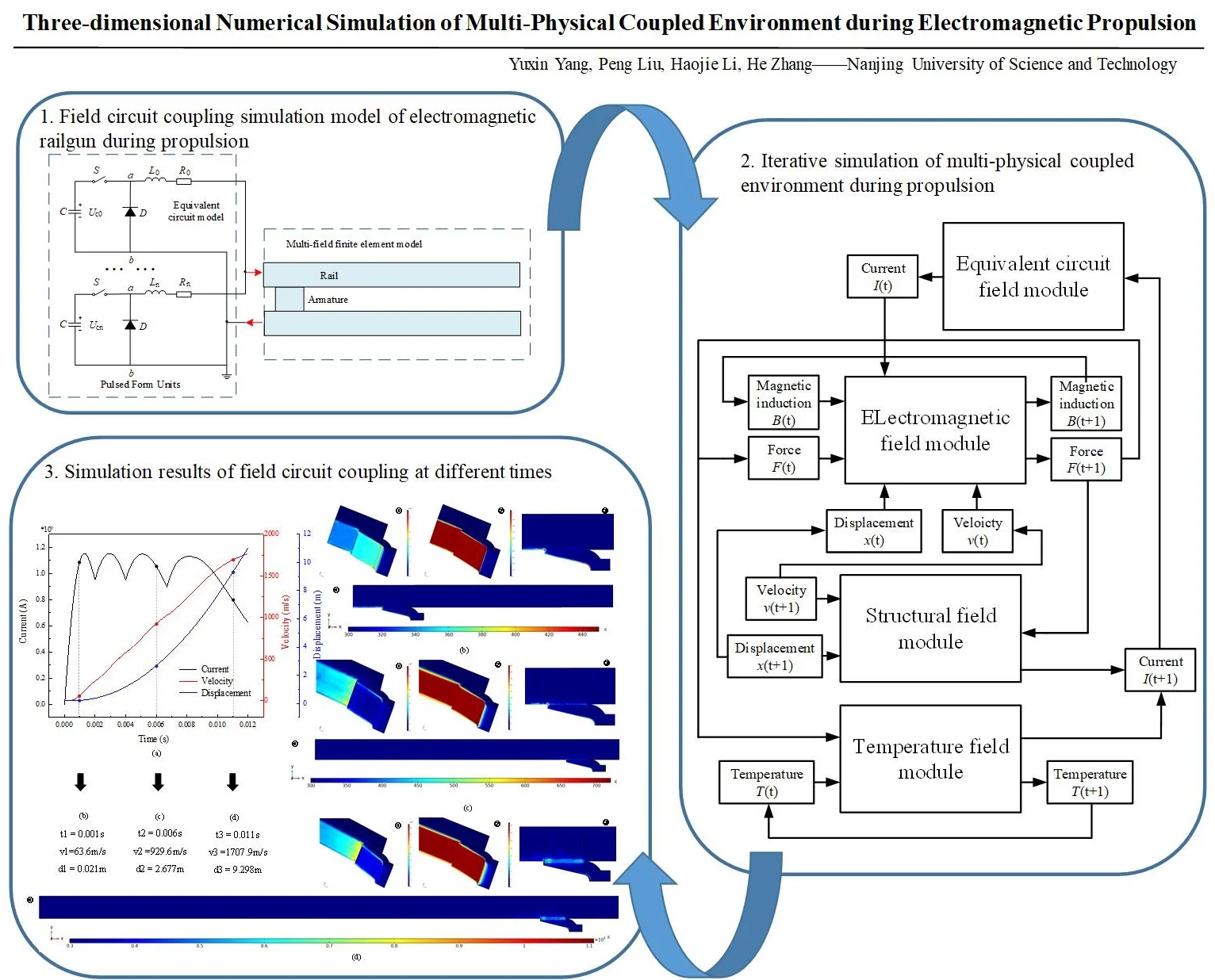
Electromagnetic propulsion technology is a new propulsion technology which uses electromagnetic force to push objects into high or ultra-high speed. However, during propulsion, the armature and launch load are affected by harsh multi-physics environment. The coupled effect was often ignored or over idealized in previous numerical simulations, which leads to large errors between simulation and experiment. In this paper, a three-dimensional multi-physics coupling environment simulation model is established. The distribution of electromagnetic field, structure field and temperature field in armature from static to high speed are effectively calculated. Moreover, the coupled effect between physical fields and the influence of key parameters on the simulation results are revealed. In conclusion, this model can reproduce the physical field distribution of armature and rail during electromagnetic propulsion. The time-varying resistance and inductance and the velocity skin effect (VSE) are the key parameters affecting armature movement. This method reveals a feasible path for the simplification of multi-physical model and the mitigation of extreme environment.

Three-dimensional numerical simulation of multi-physical coupled environment during electromagnetic propulsion

Highlights

The iterative calculation of circuit and multi-physical fields is realized by using the method of time sequence circuit model. The measured value or equivalent value is no longer required for the input current. Compared with the method of equivalent current and three-step current, the higher accuracy is obtained.
The VSE changes the distribution of current density and magnetic induction between the armature and the rail. This phenomenon leads to the concentrated distribution of current density and magnetic induction on the armature tail. Moreover, the dynamic characteristics are also influenced, and become more obvious with the increase of velocity.
The thermal field is mainly contributed by joule heat and friction heat. The VSE forms a hot spot in the contact area of armature tail, and the temperature is as high as 1200 K. Meanwhile, the effect of friction heat cannot be ignored. With the increase of the velocity, the hot line between the rail and the armature becomes more obvious.

1. Introduction

As a new type of launching platform, electromagnetic railgun has the characteristics of high initial velocity, low pollution and large muzzle kinetic energy compared with conventional platform [1-3]. It can thrust the carrier into 2000 m/s or higher speed in a few milliseconds, which can easily break through the speed limit of traditional chemical energy platform [4]. However, during the launch time, the in-bore harsh multi-physical field environment is one of the factors restricting its development [5]. The electromagnetic force is produced by the interaction of in-bore strong magnetic field and current flowing through armature, which promotes the high speed movement of armature and launch load [6]. The transient electromagnetic field and force field produce Joule heat and friction heat respectively. It will affect the conductivity of conductors, which affect the contact status between rails and armature [7]. Therefore, it is of great importance to study the multi-physics coupling effects and analysis method for better designing the launch load system.

The sliding electrical contact between armature and rails during launch has always been the main problem restricting the calculation of three-dimensional transient electromagnetic force of electromagnetic launcher [8]. Hsieh et al. [9] developed a special simulation software EMAP3D for electromagnetic propulsion process research. The magnetic diffusion process of moving conductor was described by Lagrange equation, and the coupling analysis of electromagnetic field, force field and temperature field was realized. Based on the hybrid finite element method and boundary element method, Lin Q. H. et al. [10] established the simulation model of electromagnetic field and temperature field, and realized the multi-physical field coupling analysis with finite element software. Yin et al. [11] proposed a two-dimensional multi-physics field coupling method based on magnetic diffusion method. In [12], it has been proved that the two-dimensional model can basically restore the current density and flux density distribution between the rails and armature during electromagnetic propulsion, and effectively reproduce the influence of velocity skin effect (VSE) on magnetic diffusion. However, it is impossible to quantitatively obtain the distribution of physical parameters during launch, as the height of rails and armature was ignored. The two-dimensional model with infinite rail’s height obviously overestimates the speed. In order to obtain more realistic estimation, the authors [13] assume that the armature acceleration is proportional to the current density at any time, and the final function of the calculation speed is calculated. Therefore, in order to reproduce the multi-physical field environment distribution more accurately, the establishment of three-dimensional simulation model is necessary. Gong and Li et al. [14, 15] gave the internal current distribution of the conductor under the three-dimensional rails and armature model, but large-scale meshing was needed to ensure the accuracy of the solution.

The above models used the three-step current or equivalent current as the input, while ignoring the ripple effect caused by capacitor sequential discharge and the transient changes of resistance and inductance during the armature’s movement. Compared with these two methods above, the equivalent circuit simulation method is another solution method. Based on the static electrical characteristics of the system, various physical processes are represented in the form of electrical parameters to realize the whole process simulation. In [16], the discharge curve was simulated by the energy storage capacitor bank, but the friction between the rail and the armature was not considered, resulting in certain errors. In [17, 18], the current curve measured by Rogowski-coil in experiment was used as the input current. Although this method is reliable, it means that the simulation model under each working condition needs corresponding test, which brings a certain simulation cost. In [19], the equivalent circuit model of electromagnetic railgun was established. Combined with the dynamic equation established by the program, the voltage drop generated by the inductance and resistance was serialized into the main circuit. However, this method ignores the influence of VSE.

In this paper, the three-dimensional simulation model and transient circuit model are combined to study the coupled effect between force field, electromagnetic field and temperature field during electromagnetic propulsion. According to the magnetic diffusion and heat conduction equation, a three-dimensional multi-physical field coupling model is established. Firstly, the circuit model is established to calculate the initial input current. Then, the secondary development of the commercial software realized the simulation of armature’s movement from static to high speed, which can obtain the dynamic simulation results of magnetic, current and heat distribution. Furthermore, the magnetic field diffusion of the armature and launch load is solved based on the Biot-Savart’s law. Finally, the key parameters affecting the simulation results are analyzed.

2. Theoretical model of multi-physical field environment during electromagnetic propulsion

The multi-physical field environment during propulsion is closely related to the movement of the armature. In this section, the equivalent circuit model is established to simulate the pulse current at each time. During launch, the pulse current passes through the rails and armature and generates the magnetic field. The interaction between magnetic field and current produces electromagnetic force. The force field includes the transient stress field and the transient dynamic field. It is assumed that the launch load is stationary relative to the armature, and only the transient dynamic field is considered. For the temperature field, it is mainly caused by the joule heat and the friction heat. This section will analyze the quasistatic physical model, and write programs to achieve Iterative multi-physical field coupling model.

2.1. The input current model

Nowadays, the energy supply system of electromagnetic railgun is mainly consisting of multiple capacitor banks. The equivalent circuit model of electromagnetic launch system is shown in Fig. 1. The capacitor bank is composed of $n$ numbers of capacitor energy storage modules. One or more capacitor banks are connected to the confluence plate at the tail of the electromagnetic launcher. The rails can be equivalent to inductance $L_{r}$ and resistance $R_{r}$ varying with time, the armature can be simplified to resistance $R_{a}$ .

Fig. 1Equivalent circuit model of electromagnetic propulsion process

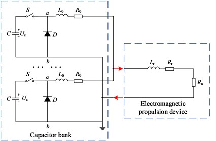
The inductance and resistance in the whole discharging circuit are composed of capacitor group and electromagnetic launcher. The capacitor group is composed of multiple encapsulated sub-circuit modules, and each module is composed of different number of capacitor modules. The appropriate input current is realized by controlling the trigger time of different sub-circuit switches. The inductance and resistance in the electromagnetic launcher will change with the movement of the armature, thus affecting the current at the subsequent time [20].

During the RLC circuit discharge, $i = - C \cdot d U_{c} / d t$ represents the input current, $U_{R} = R i = - R C d U_{c} / d t$ represents the voltage at both sides of the resistance, $U_{L} = L d i / d t = - L C d^{2} U_{c} / d t^{2}$ represents the voltage at both sides of the inductance. According to Kirchhoff 's law, there are:

1

L C \frac{d^{2} U_{c}}{d t^{2}} + R C \frac{d U_{c}}{d t} + U_{c} = 0 .

By solving capacitor voltage and loop current, the time of maximum current is $t = t_{1} = γ / ω$ . So the discharge current of single capacitor bank is as follows:

2

i = \{\begin{array}{l} \frac{U_{0}}{ω L} e^{- δ t} s i n (ω t), & (0 \leq t \leq t_{1}), \\ I_{0} e^{- R (t - t_{1}) / L}, & (t \geq t_{1}), \end{array}

where $U_{0}$ is the initial charging voltage of capacitor, and $ω = \sqrt{1 / L C - (R / 2 L)^{2}}$ , $R = R_{0} + R a + R r$ , $L = L_{0} + L_{r}$ , $δ = R / 2 L$ , $I_{0} = (U_{0} / ω L) \cdot e^{- δ t_{1}} s i n ω t_{1}$ . $R$ is the total resistance in the circuit, mainly including the internal resistance of the line and the real-time resistance of rails and armature during movement. The resistance is related to the moving distance of the armature, and the resistance gradient of the rails is usually taken as 0.1 mΩ/m [21]. $L$ is the total inductance in the circuit, including load inductance and real-time inductance. The inductance is also related with the movement of the armature. Generally, the rails’ inductance gradient are 0.51 μH/m [22]. Therefore, the equation of the discharging multiple capacitor banks is:

3

i_{a} = \{\begin{array}{l} i_{1}, & 0 \leq t \leq t_{o 1}, \\ i_{1} + i_{2}, & t_{o 1} \leq t \leq t_{o 2}, \\ \cdot \cdot \cdot & \cdot \cdot \cdot \\ i_{1} + i_{2} + \cdot \cdot \cdot + i_{n}, & t_{o n - 1} \leq t \leq t_{o n} . \end{array}

2.2. Three-dimensional magnetic diffusion model of electromagnetic propulsion process

As the wavelength of input current is larger than the size of the railgun. The displacement current can be ignored. It is studied as a quasi-static system. According to the differential form of Maxwell equation and the Ohm’s law:

4

\nabla^{2} H = σ μ_{0} \frac{\partial H}{\partial t} - σ μ_{0} \nabla \times (v \times H) .

In three-dimensional calculation, it is assumed that there is no ferromagnetic conductor in the rail and armature, and the conductivity and permeability are independent of time $t$ , then $B$ is used instead of $H$ , and the magnetic diffusion equation of the conductor in the three-dimensional model is:

5

\frac{\partial B}{\partial t} - \frac{1}{σ μ_{0}} (\frac{\partial^{2} B}{\partial x^{2}} + \frac{\partial^{2} B}{\partial y^{2}} + \frac{\partial^{2} B}{\partial z^{2}}) + v_{x} \cdot \frac{\partial B}{\partial x} = 0,

where $v_{x} \cdot \partial B / \partial x$ is the velocity diffusion term. Assuming that the armature is stationary and the rail has $x$ -axis reverse velocity relative to the armature, the magnetic diffusion equation in the armature region can be expressed as:

6

\frac{\partial B}{\partial t} - \frac{1}{σ μ_{0}} (\frac{\partial^{2} B}{\partial x^{2}} + \frac{\partial^{2} B}{\partial y^{2}} + \frac{\partial^{2} B}{\partial z^{2}}) = 0 .

The magnetic diffusion equation of armature and rail is solved by setting boundary conditions and initial value $B$ , and the current density values in $x$ -, $y$ - and $z$ -axis are obtained as follows:

7

j_{x} = \frac{1}{μ_{0}} (\frac{\partial B_{z}}{\partial y} - \frac{\partial B_{y}}{\partial z}), j_{y} = \frac{1}{μ_{0}} (\frac{\partial B_{x}}{\partial z} - \frac{\partial B_{z}}{\partial x}), j_{z} = \frac{1}{μ_{0}} (\frac{\partial B_{y}}{\partial x} - \frac{\partial B_{x}}{\partial y}) .

Ignoring the magnetic induction intensity of the rails and armature in the $x$ -, $y$ -axis, the current density in $x$ -, $y$ - and $z$ -axis are:

8

j_{x} = \frac{1}{μ_{0}} \frac{\partial B_{z}}{\partial y}, j_{y} = - \frac{1}{μ_{0}} \frac{\partial B_{z}}{\partial x}, j_{z} = 0 .

Since the input current is a low-frequency current, the generated magnetic field is similar to a stable magnetic field. Assuming that the package of the projectile is made of non-metallic materials, the magnetic induction at the inspection point of the launch load is calculated by using Biot-Savart’s law:

9

B (r) = \frac{μ_{0}}{4 π} \int \frac{J (r^{'}) \times (r - r^{'})}{{|r - r^{'}|}^{3}} d V (r^{'}),

where $V$ is the current distribution area, $r^{'}$ is the vector diameter of the source point (current element $J d V$ ), $r$ is the vector diameter of the field point. Therefore, the magnetic field distribution in front of the armature can be calculated according to the vector diameter of the source point and the solution point by solving the internal current density of the rails and armature.

The magnetic flux density generated from the source point of the rails’ surface to the central axis is:

10

d B = \frac{μ_{0} J_{v 1}}{4 π R^{3}} [(y_{0} - y) d x d y d z e_{z} - (z_{0} - z) d x d y d z e_{y}],

11

B_{v y 1} = \frac{μ_{0} J_{v 1}}{4 π} \int_{L_{0}}^{L_{1}} \int_{s / 2}^{s / 2 + δ} \int_{- h_{r} / 2}^{h_{r} / 2} \frac{z - z_{0}}{[(x_{0} - x)^{2} + (y_{0} - y)^{2} + (z_{0} - z)^{2}]^{3 / 2}} d x d y d z,

12

B_{v z 1} = \frac{μ_{0} J_{v 1}}{4 π} \int_{L_{0}}^{L_{1}} \int_{s / 2}^{s / 2 + δ} \int_{- h_{r} / 2}^{h_{r} / 2} \frac{y_{0} - y}{[(x_{0} - x)^{2} + (y_{0} - y)^{2} + (z_{0} - z)^{2}]^{3 / 2}} d x d y d z,

where $h_{r}$ is the height of the rail, $δ$ is the skin depth, $L_{0}$ is the initial position of rail, $L_{1}$ is the axial length of armature.

The magnetic flux density generated from the source point of each surface of the armature to the central axis is:

13

B_{a x z 1} = \frac{μ_{0} J_{a x 1}}{4 π} \int_{- l_{t}}^{- l_{t} + l_{c}} \int_{k x - k x_{A} + y_{A}}^{s / 2} \int_{- h_{a} / 2}^{h_{a} / 2} \frac{y_{0} - y}{[(x_{0} - x)^{2} + (y_{0} - y)^{2} + (z_{0} - z)^{2}]^{3 / 2}} d x d y d z,

14

B_{a x y 1} = \frac{μ_{0} J_{a x 1}}{4 π} \int_{- l_{t}^{}}^{- l_{t} + l_{c}} \int_{k x - k x_{A} + y_{A}}^{s / 2} \int_{- h_{a} / 2}^{h_{a} / 2} \frac{z - z_{0}}{[(x_{0} - x)^{2} + (y_{0} - y)^{2} + (z_{0} - z)^{2}]^{3 / 2}} d x d y d z,

where $h_{a}$ is the height of the armature, $δ$ is the skin depth, $L_{0}$ is the initial position of rail, $L_{1}$ is the axial length of armature.

2.3. Three dimensional dynamic model of armature

The force of armature can be expressed according to Newton’s second law:

15

m \frac{d^{2} x_{m}}{d t^{2}} = f_{x} - f_{r},

where $x_{m}$ is the displacement of armature, $f_{x}$ is the axial electromagnetic force on the armature, $f_{r}$ is the friction force on the armature.

According to the electromagnetic propulsion equation, the electromagnetic force on the armature can be expressed as:

16

f_{p} = \frac{1}{2} L^{' I^{2}} = B I s .

The axial electromagnetic force can be expressed as:

17

f_{x} = B I \frac{l {}_{c}}{c o s α} = \frac{1}{2} \cdot \frac{L^{' I^{2}}}{s} \cdot \frac{l {}_{c}}{c o s α} .

The friction is directly proportional to the pressure of the armature on the rails:

18

f_{r} = μ_{f r} (f_{n} + f_{y}) .

In the structural field, the electromagnetic propulsion received by the armature is essentially provided by the Lorentz force, which is mainly divided into the axial propulsion of the armature $f_{x}$ and the component force to the rail $f_{y}$ :

19

f_{x} = - \int_{v_{a}} B j_{y} d v, f_{y} = \int_{v_{a}} B j_{x} d v .

2.4. Three dimensional thermal diffusion model

According to Fourier’s law and thermal equilibrium law, the three dimensional thermal diffusion equation is:

20

ρ c \frac{\partial T}{\partial t} \cdot d Ω - [\nabla \cdot (k \nabla T)] \cdot d Ω = Q_{a} + Q .

The first item of the right type is the heat generated by Joule heat, and the second item is the heat generated by friction heat.

The joule heat of rails and armature is:

21

Q_{a} = \{\begin{array}{l} \frac{j_{x}^{2} + j_{y}^{2}}{σ_{r}}, \\ \frac{j_{x}^{2} + j_{y}^{2}}{σ_{a}} . \end{array}

The friction heat is:

22

Q_{s} = μ_{f r} (P + \frac{f_{l, y}}{S_{b c}}) v .

2.5. Multi-physical field coupling simulation model

The electromagnetic propulsion process is divided into a large number of microseconds in sequence. In a single time period, the circuit simulation module is used to assign capacitor bank parameters and trigger threshold settings. Then the input current is introduced into the quasi-static electromagnetic model to calculate the electromagnetic field. The variation of magnetic flux density and current density is simulated, and the results are introduced into the mechanical model to update the velocity and displacement. Finally, the results of electromagnetic model and mechanical model are introduced into the thermal model to update the temperature distribution. The last time solution of the previous time period is taken as the initial value of the next time period for iteration to realize the simulation of the whole propulsion process. According to the multi-physical field simulation model, the current distribution, magnetic field distribution, temperature distribution and velocity can be obtained.

3. Multi-physical coupling simulation of electromagnetic propulsion process

In this section, the simulation model is established based on the magnetic field module, PDE module, structural mechanics model, solid heat transfer module and circuit module in the commercial software COMSOL Multiphysics. On this basis, the secondary development is carried out, and the multi-module coupling operation is realized by programming.

3.1. Simulation of capacitor discharge circuit

According to the pulse power structure in Fig. 1, the circuit simulation module is used to build the simulation circuit. The capacitance value $C$ is 2 mF, the initial charging voltage $U_{0}$ is 9.5 kV, the wave-modulation inductance $L_{0}$ is 48 μH, the line internal resistance $R_{0}$ is 10 mΩ, the load equivalent inductance $L_{1}$ is 2 μH, and the load equivalent resistance $R_{1}$ is 20 mΩ. The package sub-circuit modules P01 to P04 represent four capacitor banks. The number of pulse power modules and trigger time of each capacitor bank are shown in Table 1. The charging voltage of each PFU module is 9.5 kV.

Fig. 2Multi-physical field coupling simulation model

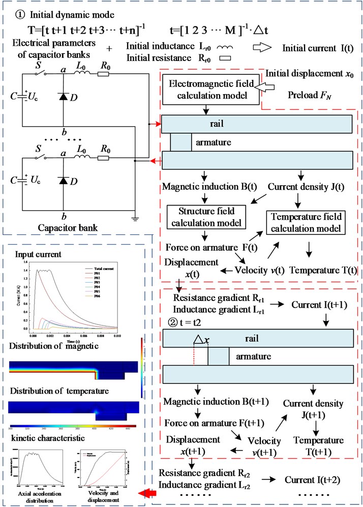
The equivalent resistance of each transmission cable is 7 mΩ, and the equivalent inductance is 0.6 μH. The resistance and inductance values in armature and rail are determined by the calculation of structural mechanics and PDE module in the following part. The total displacement of armature position is obtained by adding the calculated displacement and the initial displacement. The resistance gradient of the rail is 0.1 mΩ/m, and the inductance gradient is 0.51 μH/m for calculation. The voltage drop caused by the increment of inductance and resistance is calculated and introduced into the main circuit to output the current value at the next stage. With the iteration, the current distribution of electromagnetic propulsion is obtained.

Table 1Basic size and style requirements

Capacitor group number	Number of PFU modules	Trigger time (ms)
P01	28	0
P02	5	2.05
P03	4	4.05
P04	3	6.75

3.2. Multi-physics coupling simulation

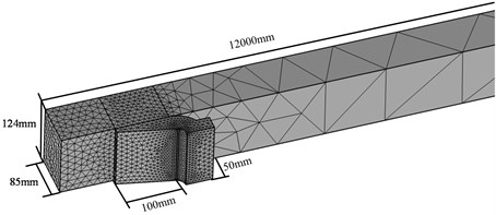
The parameters of rail and armature are constructed according to the model in [23]. The height of rail is 124 mm, the width is 85 mm, and the length is 12000 mm. The commonly used U-shaped armature is selected for armature, and the total width is 100 mm. The 1/2 model in Fig. 3 is 50 mm, and the contact area between armature and rail is 124 mm×100 mm. The rail and armature are divided by tetrahedral mesh. In order to reduce the calculation amount, the adaptive mesh is adopted. The mesh of armature area, the back side of rail and the contact area is densely set. Since the influence of front-end position is small, the mesh is sparse.

Fig. 3A schematic diagram of a vibration separator

The density, conductivity, relative permeability, thermal conductivity and specific heat capacity of rails and armature are set in Table 2.

Table 2Simulation parameter

Parameter	Value
Density of rail	8900 kg/m³
Electric conductivity of rail	4.5×10⁷ S/m
Relative permeability of rail	1
Thermal conductivity of rail	386 J/kg/K
Specific heat capacity of rail	397 W/m/K
Density of armature	2800 kg/m³
Electric conductivity of armature	3.5×10⁷ S/m
Relative permeability of armature	1
Thermal conductivity of armature	880 J/kg/K
Specific heat capacity of armature	237 W/m/K
Coefficient of sliding friction	0.02
The mass of armature and load	11 kg

Definite solution condition:

(1) Initial magnetic induction of rail and armature is $B_{0} = 0$ . The initial temperature is $T_{0} =$ 300 K.

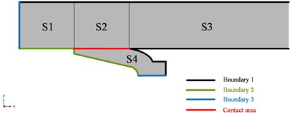
(2) In order to intuitively represent the division of boundary conditions, the boundary conditions are shown in the $X O Y$ plane. Since the rail and armature are symmetrical about the center of $x$ -axis, the 1/2 model is used for analysis. When the armature slides at a high speed relative to the rail, the VSE will be caused, so that the magnetic field and current are concentrated on the inner edge of the guide rail and the rear edge of the armature. The boundary 1 are set as $B = 0$ . The boundary 2 is set as $B = μ j$ , where the current line density is $j = I / h$ , $I$ is the input current, $h$ is the rail height. The left rail’s boundary 3 is set as $\partial B / \partial x = 0$ , the armature’s boundary 3 is set as $\partial B / \partial y = 0$ .

Fig. 4Boundary setting

4. Analysis of numerical simulation results

The pulse current obtained by calculation is shown in Fig. 5(a). It can be found that the total current synthesized by the sequential discharge of four pulse capacitors, and the trigger setting time of each pulse valley is close to that of the capacitor bank. In the simulation, the peak current reaches 1.15 MA, and the duration is 12 ms. Pulse current mainly formed three steps, the first step is the rising period, the time is 0-0.1 ms, the current is mainly provided by the first capacitor bank, the rising trend is close to sine function. The second step is the platform period, the time is 0.1-0.9 ms, and the current is provided by all capacitor banks. The current curve in this step forms multiple pulse peaks due to the different trigger time. The last step is the drop period, which is synthesized by the discharge phases of multiple capacitor banks.

Fig. 5The armature position and temperature distribution at different time points electromagnetic propulsion process

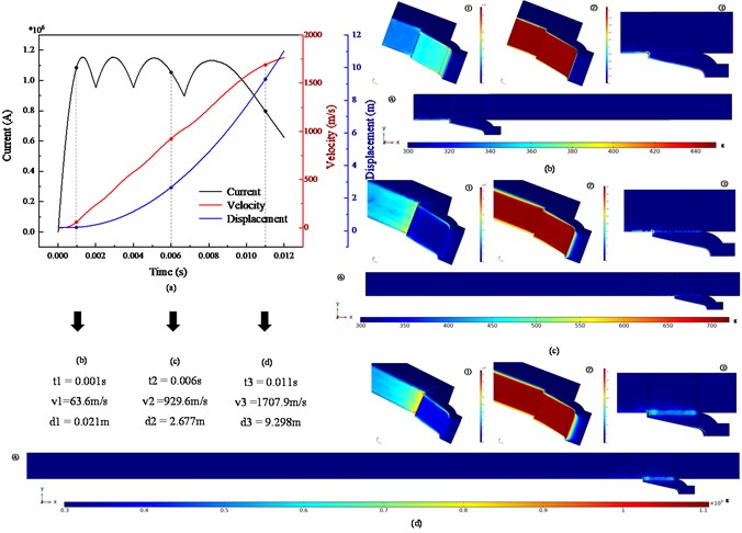
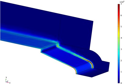
The $t_{1} =$ 0.001, $t_{2} =$ 0.006 s, $t_{3} =$ 0.011 s are selected to comparison. The current density distribution at each time is shown in Figs. 5(a1)-(c1). It can be seen that the current density is mainly distributed on the surface of the rail and the armature, the contact area between the rail and the armature. Due to the skin effect, the current density at the armature edge is large. With the increase of velocity, the peak current density is mainly distributed in the inner contour of the armature and the contact area between the armature and the rail, and the peak current density reaches about 1.2×10¹⁰A/m², as shown in Fig. 5(c1) and Fig. 5(d1). Moreover, the peak current density is multiple relative to that in other regions, which is consistent with the simulation results in [24]. The reason for this phenomenon is the combined action of skin effect and velocity skin effect.

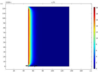
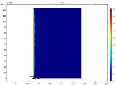
Figs. 5(b2) -(d2) represent the distribution of magnetic induction at each time. It can be found that the magnetic induction is mainly distributed in the inner surface of the rail and armature, and the peak value reaches 20 T. From the $y$ - $z$ plane section, there is a shallow diffusion depth near the armature. The VSE resulting in current concentration in the tail of the armature. As shown in Fig. 5(d), the armature velocity reaches 1680 m/s at 11 ms, and the magnetic induction in the inner surface of the armature gradually spreads forward with time.

Fig. 5(b4)-(d4) show the temperature response of the armature and rail at three moments, and the calculation accuracy is sufficient to simulate the millimeter-level or even more precise movement in the initial propulsion process. At the initial time, the temperature is mainly distributed on the inner surface of the armature and the rail. The temperature mainly due to joule heat generated by the current density, and a hot spot is formed at the contact point between the armature tail and the rail, with the peak temperature reaching 440 K. Then the speed increases and the friction heat ratio increases gradually. The hot line is formed on the contact surface of the armature and the rail. The temperature reaches 450 K and the peak temperature of the hot spot reaches 700 K. In Fig. 5(d3), the temperature on the hotline is 600 K and the temperature on the hot spot is 1100 K. It can be seen that the initial supply of temperature during electromagnetic launch is mainly provided by Joule heat generated by large current. With the increase of velocity, the VSE appears. The heat energy is mainly concentrated on the contact point between armature tail and rail, and there is also a high temperature distribution on the contact surface.

Fig. 6Axial and radial acceleration distribution of armature during propulsion

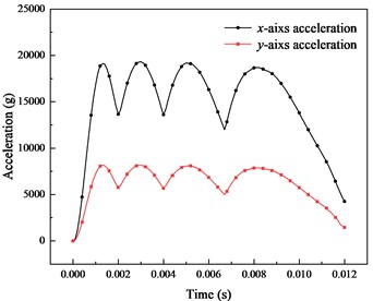
a) Acceleration

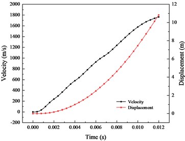
b) Velocity

The axial and radial acceleration distribution obtained by Eq. (19) in Fig.6(a). The axial peak acceleration is 19000 g, and the radial peak acceleration is 8000 g. The radial pressure is expressed in the form of acceleration for comparison with the axial acceleration. The radial pressure is converted into friction force during propulsion, which affects the movement of the armature. The axial acceleration lasted about 8 ms in the peak stage, and the maximum difference was 6000 g. The velocity and displacement obtained after integration are shown in Fig. 6(b), For the whole propulsion process, the armature is accelerated to nearly 1700 m/s in just 12 ms, with the propulsion distance of only 11 m.

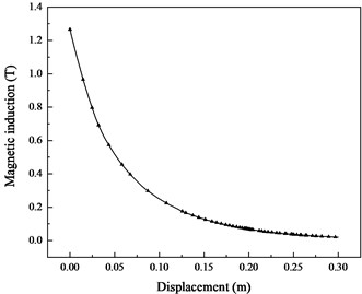
Fig. 7The distribution of magnetic induction at the position away from the axis of the armature

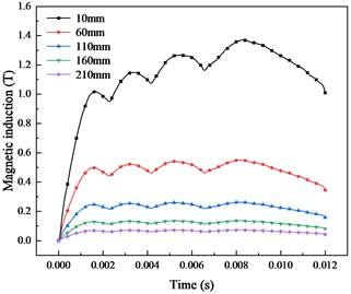
a) Different position

b) Peak value

Based on Eq. (9-14), the magnetic field distribution of central axis position is solved, which provides a reference for the design and protection of precision circuit components. As shown in Fig. 7, the simulation results show that the magnetic induction decreases exponentially with the increase of the distance from the armature. The peak magnetic flux density at 10 mm from the armature reaches 1.4 T, while the magnetic flux density at 210 mm is only 0.1 T. Therefore, the position of the magnetic sensitive device is as far away from the armature as possible, and the direction is parallel to the magnetic field direction as far as possible, so that the influence of the pulse magnetic field on the device is minimized.

5. Comparison and discussion

The main influencing factors in the complex environment are the velocity skin effect and the changes of resistance and inductance during movement. The elaboration and demonstration of their influence are discussed in the following parts.

5.1. Influence analysis of input current

The change of resistance and inductance caused by the moving armature during launch. The actual current waveform is formed by controlling the sequential discharge of multiple capacitor banks. The equivalent current method is used to simulate the current during launch [25], and the influence of time-varying circuit parameters of the launch device is ignored. The equation of the current can be seen in Eq. (23):

23

I = \{\begin{array}{l} I_{0} s i n ω t, & 0 \leq t \leq t_{1}, \\ I_{0}, & t_{1} < t \leq t_{2}, \\ I_{0} e^{- \frac{t - t_{2}}{τ}}, & t_{2} < t \leq t_{3} . \end{array}

In this section, the equivalent resistance and inductance is changed with the velocity and displacement of the armature, and the coupling of the structural field and the circuit simulation model is realized. The simulation results are compared with three-step current and those without considering the transient changes of resistance and inductance, as shown in Fig. 8.

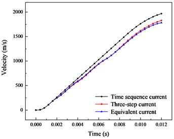
The method in this paper (time sequence current) is compared with two common equivalent input current methods. One is the equivalent current (without considering the moving armature), and the other is simplified three-step current. The comparison between the current curve obtained in this paper and the other two methods is shown in the Fig. 8.

At the rising step of the current, the variation characteristics of the three input currents are basically the same. In the platform step, the difference between the three-stage current and the method in this paper is the largest. It can be found that the error between the peak value and valley value reaches about 0.2 MA. The capacitor bank discharge sequence generated by the ripple phenomenon was ignored with the method of three-step current. The change of resistance and inductance was ignored with the method of the equivalent current, and the difference is also existed. The amplitude at the initial step is slightly larger, and is slightly smaller at the later step.

Fig. 8Comparison of the equivalent current and time sequence discharging current

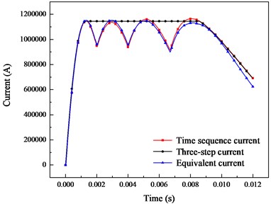
Fig. 9Comparison of dynamic characteristics between time sequence, three-step and equivalent current

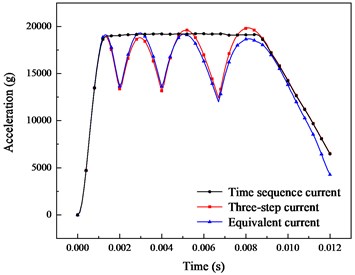
a) Acceleration

b) Velocity

The dynamic characteristics calculated by using the three methods are shown in the Fig. 9. It can be found that the acceleration value calculated by three-step current cannot show the ripple phenomenon in sequential current calculation. The maximum difference in acceleration is 5000 g in 1-9 ms, while the result of three-step current is a stable waveform. The equivalent current has little difference from the time sequence current. The value in 1-4 ms is larger, and the value in 4-12 ms is smaller, with an error of 1000 g. The comparison of velocity is shown in Fig. 9(b). The velocity obtained by the three-stage current is the largest different from that in this paper, the value is up to 260 m/s, and the value between equivalent current and that in this paper is up to 50 m/s.

5.2. Influence of VSE on simulation results

The movement of the armature relative to the rails cause the VSE, which takes the magnetic line out of the contact area, thus counteracting the slow magnetic diffusion into the conductive material of the rail and armature. In this paper, the partial differential equations of rail and armature are established to simulate the relative movement, and the results of each step are iterated to the next step to realize coupling. The velocity skin effect is the main factor affecting the current distribution during launch. In the previous discussion, it can be found that the magnetic field, current and temperature distribution of high-speed motion are significantly different from those of low-speed and static processes.

Fig. 10The distribution of current density and magnetic induction in stationary state

a) Magnetic induction

b) Current density

Fig. 11The distribution of current density and magnetic induction in moving state

a) Magnetic induction

b) Current density

As shown in Fig. 10, the magnetic flux density distribution at the $x$ - $y$ interface of the contact area between the rail and the armature, and the current density distribution between the armature and the rail. The distribution of magnetic flux density and current density under the influence of velocity, as shown in Fig. 11. It can be found that in the static process, the diffusion depth of magnetic flux density is 14 mm, and gradually decay. During the movement, the flux density concentrates on the surface and the diffusion depth is only 2.5 mm. The static current density is mainly distributed in the rail and the armature edge, and reaches the highest at the boundary position of the armature throat. The distribution of current density in the motion process is significantly different from that in the static process. When the VSE is not considered, the current density is distributed on the rail. The peak current density is affected by the skin effect, and the peak current density is concentrated in the armature and the rail corner, reaching 7×10⁹A/m². When considering the VSE, the current density on the rail surface increases to 7×10⁹A/m², and the peak current density at the contact position between the rail and the armature reaches 9×10⁹A/m². It can be found that the velocity skin effect will lead to the concentrated distribution of current density and the surface of the rail and the contact position with the armature, and form a concentrated distribution. It mainly affects the current density distribution on the rail and the current density distribution at the connection position between the rail and the armature.

The dynamic characteristics of armature considering and not considering VSE are compared in Fig. 12. It can be found from Fig. 12(a) that the $x$ -axis acceleration distribution obtained by the two simulation models is basically coincident within 0.002 s. With the increased of the velocity, the distribution of current density and magnetic induction are affected by VSE. Thus, the electromagnetic force is changed. The error between two simulation models is gradually increased in 0.004-0.012 s, and the peak error reaches about 4000 g. In contrast, the error of $y$ -axis acceleration obtained by the two simulation methods is relatively low, indicating that VSE has little effect on axial pressure. The comparison of velocity between the two simulation methods is shown in Fig. 12(b). The maximum velocity error reaches about 150 m/s. Therefore, the VSE should be considered in the simulation.

Fig. 12Dynamic characteristics of armature considering and not considering VSE

a) Acceleration

b) Velocity

5.3. Experimental verification

In order to verify the reliability of the simulation method proposed in this paper, we compare the simulation and experimental results in [26].

The influence of VSE is simulated by changing the rails’ structure model and the contact area between rails and armature in the reference. Moreover, the electromagnetic field and structural field environment during launch are measured by the projectile-borne storage testing system. The method in the reference did not realize the magneto-mechanical coupled effect during launch. The electromagnetic field and structural field were not calculated iteratively, and the influence of field-circuit coupling was not considered.

Fig. 13Comparison of velocity and displacement between method in reference, this paper and experiment

a) Velocity

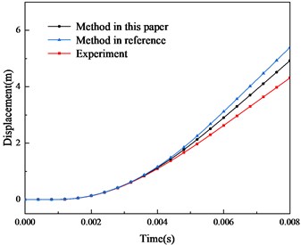
b) Displacement

Based on the theoretical model and numerical simulation method in this paper, the input current, structure and material parameters of armature and rails in the reference are established. The differences between the two simulation and experiment results are compared and analyzed in Fig. 13 and Fig. 14. It can be found that the simulation results in this paper cannot completely reproduce the experiment results, as some simplified factors in the simulation and the non-ideal factors in the experiment. However, compared with the simulation results in the reference, the error between the simulation and the experiment results becomes smaller. The error between the simulation of this paper and the experiment is reduced to 100 m/s in velocity and 0.5 m in displacement. This also reflects the reliability of the method in this paper.

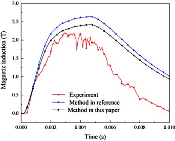
The comparison of the magnetic field distribution during launch is shown in Fig. 14. The distance between the sensors and the armature is 60 mm. According to the parameters in this paper, the magnetic induction is calculated by the simulation method in this paper, as shown in the black curve in Fig. 14. Considering the influence of ferromagnetic shell material, there is no ripple phenomenon caused by pulse timing current, and the simulation results in this paper are closer to the experiment results. The error of peak magnetic induction is reduced to 0.6 T.

Fig. 14Comparison of magnetic induction between method, experiment in reference and this paper

6. Conclusions

In this paper, the mathematical model of three-dimensional electromagnetic field, structural field and temperature field in electromagnetic launch process is established. The secondary development of finite element software is carried out to restore the current distribution, armature motion characteristics and magnetic field and temperature distribution in the electromagnetic launch process. The influence of VSE on magnetic field diffusion and current density distribution is revealed, and the magnetic field distribution in front of armature is deduced based on Biot-Savart law. The contrastive analysis of the simulation results is given and the conclusions are summarized as follows:

1) The iterative calculation of circuit and multi-physical fields is realized by using the method of time sequence circuit model. The measured value or equivalent value is no longer required for the input current. Compared with the method of equivalent current and three-step current, the higher accuracy is obtained in this paper.

2) The VSE changes the distribution of current density and magnetic induction between the armature and the rail. This phenomenon leads to the concentrated distribution of current density and magnetic induction on the armature tail. Moreover, the dynamic characteristics are also influenced, and become more obvious with the increase of velocity.

3) The thermal field is mainly contributed by joule heat and friction heat. The VSE forms a hot spot in the contact area of armature tail, and the temperature is as high as 1200 K. Meanwhile, the effect of friction heat cannot be ignored. With the increase of the velocity, the hot line between the rail and the armature becomes more obvious.

References

W. Ma and J. Lu, “Thinking and study of electromagnetic launch technology,” IEEE Transactions on Plasma Science, Vol. 45, No. 7, pp. 1071–1077, Jul. 2017, https://doi.org/10.1109/tps.2017.2705979

Publisher
J. Li, P. Yan, and W. Yuan, “Electromagnetic gun technology and its development,” (in Chinese), High Voltage Engineering, Vol. 40, pp. 1052–1064, 2014, https://doi.org/10.13336/j.1003-6520.hve.2014.04.014

Publisher
H. D. Fair, “Advances in electromagnetic launch science and technology and its applications,” IEEE Transactions on Magnetics, Vol. 45, No. 1, pp. 225–230, Jan. 2009, https://doi.org/10.1109/tmag.2008.2008612

Publisher
J. Mcfarland and I. R. Mcnab, “A long-range naval railgun,” IEEE Transactions on Magnetics, Vol. 39, No. 1, pp. 289–294, Jan. 2003, https://doi.org/10.1109/tmag.2002.805924

Publisher
H. Zhang, K. Dai, and Q. Yin, “Ammunition reliability against the harsh environments during the launch of an electromagnetic gun: a review,” IEEE Access, Vol. 7, pp. 45322–45339, 2019, https://doi.org/10.1109/access.2019.2907735

Publisher
J. P. Barber and I. R. Mcnab, “Magnetic blow-off in armature transition,” IEEE Transactions on Magnetics, Vol. 39, No. 1, pp. 42–46, Jan. 2003, https://doi.org/10.1109/tmag.2002.805855

Publisher
T. Benton, F. Stefani, S. Satapathy, and Kuo-Ta Hsieh, “Numerical modeling of melt-wave erosion in conductors [railgun armatures],” IEEE Transactions on Magnetics, Vol. 39, No. 1, pp. 129–133, Jan. 2003, https://doi.org/10.1109/tmag.2002.805871

Publisher
W. Ma, J. Lu, and X. Li, “Electromagnetic launch hypervelocity integrated projectile,” (in Chinese), Journal of National University of Defense Technology, Vol. 41, No. 4, pp. 1–10, 2019.

Search CrossRef
K.-T. Hsieh, “Hybrid FE/BE Implementation on electromechanical systems with moving conductors,” IEEE Transactions on Magnetics, Vol. 43, No. 3, pp. 1131–1133, Mar. 2007, https://doi.org/10.1109/tmag.2006.887437

Publisher
Q.-H. Lin and B.-M. Li, “Numerical simulation of interior ballistic process of railgun based on the multi-field coupled model,” Defence Technology, Vol. 12, No. 2, pp. 101–105, Apr. 2016, https://doi.org/10.1016/j.dt.2015.12.008

Publisher
Q. Yin, H. Zhang, H.-J. Li, and Y.-X. Yang, “Analysis of in-bore magnetic field in C-shaped armature railguns,” Defence Technology, Vol. 15, No. 1, pp. 83–88, Feb. 2019, https://doi.org/10.1016/j.dt.2018.07.009

Publisher
K. Dai, Y. Yang, Q. Yin, and H. Zhang, “Theoretical model and analysis on the locally concentrated current and heat during electromagnetic propulsion,” IEEE Access, Vol. 7, pp. 164856–164866, 2019, https://doi.org/10.1109/access.2019.2952981

Publisher
J. D. Powell and A. E. Zielinski, “Current and heat transport in the solid-armature railgun,” IEEE Transactions on Magnetics, Vol. 31, No. 1, pp. 645–650, Jan. 1995, https://doi.org/10.1109/20.364618

Publisher
X. Li and C. Weng, “Three-dimensional investigation of velocity skin effect in U-shaped solid armature,” Progress in Natural Science, Vol. 18, No. 12, pp. 1565–1569, Dec. 2008, https://doi.org/10.1016/j.pnsc.2008.05.024

Publisher
F. Gong and C.-S. Weng, “The effects of rail coatings on melt-wave erosion in block armatures,” International Journal of Applied Electromagnetics and Mechanics, Vol. 40, No. 4, pp. 323–331, Nov. 2012, https://doi.org/10.3233/jae-2012-1595

Publisher
Y. Guan et al., “Circuit Simulation of the Electromagnetic railgun system,” High Power Laser and Particle Beams, Vol. 26, No. 11, pp. 226–230, 2014, https://doi.org/10.11884/hplpb201426.114103

Publisher
C.-Y. Zhu and B.-M. Li, “Analysis of sliding electric contact characteristics in augmented railgun based on the combination of contact resistance and sliding friction coefficient,” Defence Technology, Vol. 16, No. 4, pp. 747–752, Aug. 2020, https://doi.org/10.1016/j.dt.2019.12.007

Publisher
B. Tang, Y. Xu, Q. Lin, and B. Li, “Synergy of melt-wave and electromagnetic force on the transition mechanism in electromagnetic launch,” IEEE Transactions on Plasma Science, Vol. 45, No. 7, pp. 1361–1367, Jul. 2017, https://doi.org/10.1109/tps.2017.2705220

Publisher
Y. Zhou, D. Zhang, and P. Yan, “Modeling of electromagnetic rail launcher system based on multifactor effects,” IEEE Transactions on Plasma Science, Vol. 43, No. 5, pp. 1516–1522, May 2015, https://doi.org/10.1109/tps.2015.2403264

Publisher
J. Liu, Y. Zhao, and X. Qin, “Releasing method for reverse charging voltage of stored energy capacitor in pulsed power supply system,” Electric machines and Control, Vol. 21, No. 8, pp. 41–47, 2017, https://doi.org/10.15938/j.emc.2017.08.006

Publisher
Jun Li et al., “Design and testing of a 10-MJ electromagnetic launch facility,” IEEE Transactions on Plasma Science, Vol. 39, No. 4, pp. 1187–1191, Apr. 2011, https://doi.org/10.1109/tps.2011.2110649

Publisher
M. Ghassemi, Y. M. Barsi, and M. H. Hamedi, “Analysis of force distribution acting upon the rails and the armature and prediction of velocity with time in an electromagnetic launcher with new method,” IEEE Transactions on Magnetics, Vol. 43, No. 1, pp. 132–136, Jan. 2007, https://doi.org/10.1109/tmag.2006.887645

Publisher
P. Du, J. Lu, J. Feng, S. Tan, K. Li, and X. Li, “Numerical simulation of dynamic launching process of electromagnetic rail launcher with electromagnetic and structural coupling,” Transactions of China Electrotechnical Society, Vol. 35, No. 18, pp. 3802–3810, 2020, https://doi.org/10.11887/j.cn.201606007

Publisher
C. Li et al., “Influence of armature movement velocity on the magnetic field distribution and current density distribution in railgun,” IEEE Transactions on Plasma Science, Vol. 48, No. 6, pp. 2308–2315, Jun. 2020, https://doi.org/10.1109/tps.2020.2990926

Publisher
X. Li, J. Lu, Y. Li, and X. Wu, “3-D numerical analysis of distribution characteristics of electromagnetic launcher projectile in-bore magnetic field,” (in Chinese), Electric machines and Control, Vol. 22, No. 8, pp. 34–40, 2018, https://doi.org/10.15938/j.emc.2018.08.005

Publisher
Y. Yang et al., “In-Bore dynamic measurement and mechanism analysis of multi-physics environment for electromagnetic railguns,” IEEE Access, Vol. 9, pp. 16999–17010, 2021, https://doi.org/10.1109/access.2021.3053255

Publisher

About this article

Received

17 September 2021

Accepted

21 November 2021

Published

25 January 2022

SUBJECTS

Dynamics and oscillations in electrical and electronics engineering

DOI

https://doi.org/10.21595/jve.2021.22215

Keywords

electromagnetic railgun

numerical simulation

multi-physics coupling

velocity skin effect

This is an open access article distributed under the Creative Commons Attribution License, which permits unrestricted use, distribution, and reproduction in any medium, provided the original work is properly cited.

Previous article in issue Previous Next article in issue Next

Research article

2023 11 25

The effect of ambient temperature on the internal ballistic overload of a large-caliber artillery projectile fuze system

Zilong Yang, Deren Kong, Chunyan Zhang

Research article

2022 08 15

The Influence of projectile shielding on the internal magnetic field during an electromagnetic launch

Yuxin Yang, Peng Liu, Haojie Li, He Zhang

Research article

2018 04 20

Numerical simulation analysis of multi-physical coupling field with abrasive flow precision polishing variable-aperture tube

Jun Ye Li, Wen Qing Meng, Bin Yu Wang, Hua Xiong, Xin Ming Zhang, Ji Kun Hou

Research article

2018 03 31

Investigation of armature-rail interaction in linear electromagnetic launcher

Justinas Račkauskas, Rimantas Kačianauskas, Markus Schneider

Y. Yang, P. Liu, H. Li, and H. Zhang, “Three-dimensional numerical simulation of multi-physical coupled environment during electromagnetic propulsion,” Journal of Vibroengineering, Vol. 24, No. 2, pp. 369–385, Jan. 2022, https://doi.org/10.21595/jve.2021.22215

Copy Extrica

Copied to clipboard!

TY  - JOUR
DO  - 10.21595/jve.2021.22215
UR  - https://doi.org/10.21595/jve.2021.22215
TI  - Three-dimensional numerical simulation of multi-physical coupled environment during electromagnetic propulsion
T2  - Journal of Vibroengineering
AU  - Yang, Yuxin
AU  - Liu, Peng
AU  - Li, Haojie
AU  - Zhang, He
PY  - 2022
DA  - 2022/01/25
PB  - JVE International Ltd.
SP  - 369-385
IS  - 2
VL  - 24
SN  - 1392-8716
SN  - 2538-8460
ER  - 

Copy Ris

Copied to clipboard!

@article{Yang_2022,
	doi = {10.21595/jve.2021.22215},
	url = {https://doi.org/10.21595/jve.2021.22215},
	year = 2022,
	month = {jan},
	publisher = {{JVE} International Ltd.},
	volume = {24},
	number = {2},
	pages = {369--385},
	author = {Yuxin Yang and Peng Liu and Haojie Li and He Zhang},
	title = {Three-dimensional numerical simulation of multi-physical coupled environment during electromagnetic propulsion},
	journal = {Journal of Vibroengineering}
}

Copy Bibtex

Copied to clipboard!

[1]Y. Yang, P. Liu, H. Li, and H. Zhang, “Three-dimensional numerical simulation of multi-physical coupled environment during electromagnetic propulsion,” Journal of Vibroengineering, vol. 24, no. 2, pp. 369–385, Jan. 2022, doi: 10.21595/jve.2021.22215.

Copy IEEE

Copied to clipboard!

Yang, Yuxin, Peng Liu, Haojie Li, and He Zhang. “Three-Dimensional Numerical Simulation of Multi-Physical Coupled Environment during Electromagnetic Propulsion.” Journal of Vibroengineering 24, no. 2 (January 25, 2022): 369–85. https://doi.org/10.21595/jve.2021.22215.

Copy Chicago

Copied to clipboard!

Three-dimensional numerical simulation of multi-physical coupled environment during electromagnetic propulsion

Abstract

Highlights

1. Introduction

2. Theoretical model of multi-physical field environment during electromagnetic propulsion

2.1. The input current model

2.2. Three-dimensional magnetic diffusion model of electromagnetic propulsion process

2.3. Three dimensional dynamic model of armature

2.4. Three dimensional thermal diffusion model

2.5. Multi-physical field coupling simulation model

3. Multi-physical coupling simulation of electromagnetic propulsion process

3.1. Simulation of capacitor discharge circuit

3.2. Multi-physics coupling simulation

4. Analysis of numerical simulation results

5. Comparison and discussion

5.1. Influence analysis of input current

5.2. Influence of VSE on simulation results

5.3. Experimental verification

6. Conclusions

References

About this article

Related Articles