Permanent displacement estimation method based on variational mode decomposition

1. Introduction

The main purpose of baseline correction of seismic acceleration records is to remove or reduce the baseline drift in the records and effectively restore the real situation of the records so as to analyze and interpret the data of seismic acceleration records more accurately. Baseline drift is the constant change or deviation of the reference level in the signal caused by a variety of factors, which may obscure or confuse the true characteristics of the seismic signal. Low-frequency noise correction is critical when processing records because low-frequency noise often masks important signal components of seismic events, resulting in the inability to derive accurate acceleration time histories.

Therefore, in order to obtain effective seismic acceleration data, scholars have conducted a lot of research and proposed various correction methods to reduce the impact of baseline drift. Graizer [1] proposed a high-order polynomial baseline correction method, which is determined by least squares fitting of strong earthquake records without weighting the part containing the main signal. Iwan et al. [2] proposed a piecewise correction method based on the hysteresis effect of the instrument sensor, which assumed that the baseline shift occurred during the strong earthquake section and the end period after the strong earthquake section, and the baseline drift within each section could be represented by constants, respectively, and then the piecewise correction was performed. Chiu [3] proposed a method of preprocessing strong vibration records with high-pass filtering and then baseline correction. Wu and Wu [4] proposed an improved baseline correction method based on the Iwan method and processed the near-field intensity vibration records of the Chi-chi MW 7.6 earthquake in 1999 and the Gongcheng MW 6.8 earthquake in 2003. The calculated results of the permanent displacement have a high agreement with the GPS coseismic displacement. Boore [5] discussed and proposed a base-line calibration scheme based on Monte Carlo and used noise models to model the variation of the base line. Chanerley and Alexander [6] propose a wavelet transform-based approach designed to correct for baseline offset and tilt and integrate it into displacement. However, these methods have certain limitations, and the VMD method adopted in this paper can not only effectively estimate the permanent displacement but also reduce the dependence on subjective judgment and realize automatic data processing.

2. Variational mode decomposition (VMD)

VMD is a signal processing method with adaptive and completely non-decreasing characteristics [7]. Its core idea is to construct and solve the constrained variational problem and realize adaptive signal decomposition by solving the optimal solution of the constrained variational model. Finally, IMF components in several different frequency bands are obtained. In the calculation of VMD, IMF is defined as a frequency modulation-amplitude modulation signal $u_k$:

where, $A_k\left(t\right)$ is the instantaneous amplitude, ${\varnothing }_k\left(t\right)$ is the instantaneous phase.

The following is the establishment process of the variational model of the VMD algorithm: First, a variational model is constructed, assuming that the sample signal is decomposed into $K$ IMF, the spectrum of different modal components is calculated through Hilbert transformation, and then the signal of different modes is modulated to a specific fundamental frequency band by the exponential function method, and finally the bandwidth of different modal components is determined by solving the L² norm. The variational model obtained is as follows:

where $u_k$ represents the $k$-th modal component of target signal $f_t$ decomposition; ${\omega }_k$ is the center frequency corresponding to $u_k$; and $\delta \left(t\right)$ is the unit impulse function. Since the constrained variational problem is generally difficult to solve, the quadratic penalty factor $\alpha$ and the Lagrange multiplication operator $\lambda$ are introduced to transform it into an unconstrained variational problem, and the following augmenting Lagrange expression is obtained:

The multiplication operator alternate direction method of multipliers is used to solve Eq. (3), and $u_k^{n+1}$, ${\omega }_k^{n+1}$ and ${\lambda }_k^{n+1}$ are constantly updated. The variational problem is transformed into a saddle point for searching the augmented Lagrange expression. Finally, the saddle point of the unconstrained variational problem is obtained, that is, the optimal solution of Eq. (1), and $K$ narrow-band IMF is obtained by decomposition. The solution to $u_k^{n+1}$ is as follows:

By using the Parseval/Plancherel Fourier isometric transform under the norm, Eq. (4) is converted from the time domain to the frequency domain, and the updated expression of the modal component a in the frequency domain is obtained:

The update expression for the center frequency can also be obtained:

where ${\omega }_k^{n+1}$ is the center of gravity of the power spectrum of $k$th modal function. The main idea of VMD is to decompose the sample signal into a set of basic mode functions; each IMF corresponds to the different frequency and time domain characteristics of the signal and is constantly updated in the frequency domain; and finally, the time domain result is obtained by Fourier transform.

3. Permanent displacement estimation based on VMD

At near-fault locations, strong ground motions may contain long-period pulse waves that cause substantial permanent ground deformation. The traditional filtering method increases the cumulative error when the acceleration record is double integrated to obtain the velocity and displacement time history, so it cannot extract the accurate ground permanent displacement from the acceleration time history. The detailed process of baseline correction in this paper is referred to in reference [8], and the basic steps are as follows:

Step 1: Utilize the VMD method to decompose the velocity time history curve into $n$$imf$ components. By analyzing the entropy values of the low-frequency components, select the component $im{f}_{d1}$ with the maximum entropy as the representative of the low-frequency component. Then, find the last zero-crossing point of $im{f}_{d1}$ and the remaining ($n-1$) $imf$ components and data before the right end of $im{f}_{d1}$ passes through the zero point are added together to form the record after the first correction.

Step 2: Take the data after the rightmost zero-crossing point of $im{f}_{d1}$ as a new record to be corrected. Repeat the first step to obtain the second corrected record. Add the second corrected record to the first corrected record to create a new corrected record.

Step 3: Similarly, consider the data after the rightmost zero-crossing point of $im{f}_{d2}$ (obtained in the previous step) as a new record to be corrected. Repeat the first step until the newly obtained record to be corrected becomes a monotonic curve or a constant term. When this condition is met, stop the iterations.

Step 4: Sum all the corrected records obtained during the iterative process to form the final corrected record. Since the final record to be corrected becomes a monotonic curve or a constant term, it can be discarded.

This paper adopts a completely automatic baseline correction method, which decomposes the seismic signal into modal functions of different frequencies, then extracts the low-frequency modal functions, and finally subtracts these low-frequency functions from the original signal. The low-frequency modal function component contains the linear trend term, which can be used for baseline correction. By this method, the permanent displacement can be obtained directly by integrating the velocity time history after obtaining the corresponding velocity pulse component.

Then, the permanent displacement obtained by this method is compared with the GPS coseismic displacement to verify its rationality and application range. In this paper, we selected the records of 32 seismic stations from the Great East Japan earthquake of March 11, 2011, which were located parallel to the fault. According to the longitude, latitude, fault, and epicenter information of each station, a spatial distribution map of these stations is made (as shown in Fig. 1).

Fig. 1Spatial distribution of seismic stations

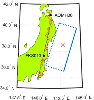
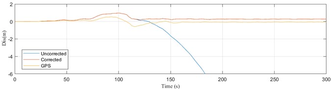
Fig. 2Estimation of permanent displacement in two directions of AOMH06 station

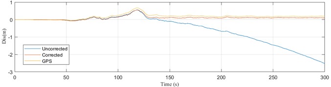
a) Estimation of permanent displacement in the EW direction of AOMH06 station

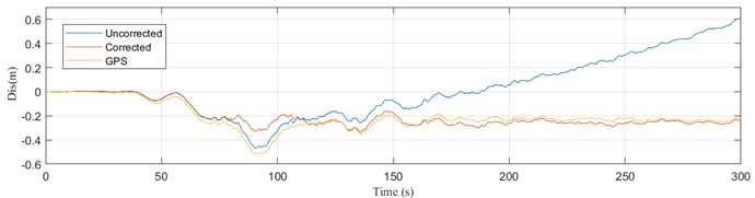
b) Estimation of permanent displacement in the NS direction of AOMH06 station

In order to directly verify the accuracy of the permanent displacement obtained by the baseline correction method in this paper, two groups of nearby strong earthquake stations in the Great East Japan Earthquake were selected to compare with GPS stations. The permanent displacement of AOMH06 and FKS013 seismic acceleration records after correction is compared with the observation results of 143 GPS station and 211 GPS station, respectively. Due to the large error in the vertical observation results of GPS stations, this paper only analyzes and compares the two horizontal directions. The spatial position of the AOMH06 station and FKS013 station as shown in Fig. 1 and the permanent positioning of the two horizontal directions obtained after correction as shown respectively in Fig. 2 and Fig. 3. It can be seen from the figure that the permanent shift obtained using the baseline correction method in this paper is consistent with the geometric shift observed by the GPS station.

Fig. 3Estimation of permanent displacement in two directions of FKS013 station

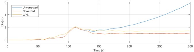
a) Estimation of permanent displacement in the EW direction of FKS013 station

b) Estimation of permanent displacement in the NS direction of FKS013 station

This method is used to correct the 32 recorded displacement time history, and their time history curves are drawn in the order of recording time in Fig. 4. In the displacement time history, it is clearly shown that the corrected time history function contains the permanent displacement information of the station. The method used in this article is reasonably feasible and works well.

Fig. 4Displacement time history of 32 stations

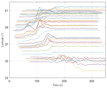
a) Displacement time history in the EW direction

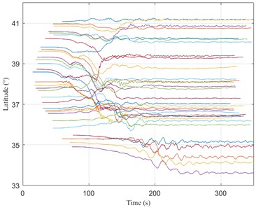
b) Displacement time history in the NS direction

4. Conclusions

This paper adopts a baseline correction method based on VMD. Compared with the traditional baseline correction method, this method is completely automatic and does not need to set any parameters in advance, which reduces the uncertainty of subjective experience on the baseline correction results. Using this method, 32 strong earthquake records of the Great East Japan Earthquake were corrected, and the permanent displacements were obtained. Two sets of data were selected and compared with the coseismic displacements of nearby GPS stations. The results show that the permanent displacement obtained after correction is in good agreement with the nearby GPS observations, which verifies the effectiveness and accuracy of the method.

References

-
V. M. Graizer, “Determination of the true ground displacement by using strong motion records,” Izvestiya, Physics of the Solid Earth, Vol. 15, pp. 875–885, 1979.
W. D. Iwan, M. A. Moser, and C.-Y. Peng, “Some observations on strong-motion earthquake measurement using a digital accelerograph,” Bulletin of the Seismological Society of America, Vol. 75, No. 5, pp. 1225–1246, Oct. 1985, https://doi.org/10.1785/bssa0750051225
H.-C. Chiu, “Stable baseline correction of digital strong-motion data,” Bulletin of the Seismological Society of America, Vol. 87, No. 4, pp. 932–944, Aug. 1997, https://doi.org/10.1785/bssa0870040932
Y.-M. Wu and C.-F. Wu, “Approximate recovery of coseismic deformation from Taiwan strong-motion records,” Journal of Seismology, Vol. 11, No. 2, pp. 159–170, Mar. 2007, https://doi.org/10.1007/s10950-006-9043-x
S. Akkar and D. M. Boore, “On baseline corrections and uncertainty in response spectrafor baseline variations commonly encounteredin digital accelerograph records,” Bulletin of the Seismological Society of America, Vol. 99, No. 3, pp. 1671–1690, Jun. 2009, https://doi.org/10.1785/0120080206
A. A. Chanerley and N. A. Alexander, “Obtaining estimates of the low-frequency ‘fling’, instrument tilts and displacement timeseries using wavelet decomposition,” Bulletin of Earthquake Engineering, Vol. 8, No. 2, pp. 231–255, Apr. 2010, https://doi.org/10.1007/s10518-009-9150-5
D. Konstantin and Z. Dominique, “Variational mode decomposition,” IEEE Transactions on Signal Processing, Vol. 62, No. 3, pp. 531–544, 2014.
D. Li et al., “Baseline correction method based on variational mode decomposition,” in The 2021 World Congress on Advances in Structural Engineering and Mechanics (ASEM21), 2021.
About this article
The authors have not disclosed any funding.
The datasets generated during and/or analyzed during the current study are available from the corresponding author on reasonable request.
The authors declare that they have no conflict of interest.