Transforming data with the arcsine distribution for random walks

Laarichi, Yassine; Elkaf, Mariem; Aloui, Amal; Rholam, Oualid

doi:10.21595/mme.2024.24105

Mathematical Models in Engineering

Browse Journal

Submit article

Published: 23 May 2024

Check for updates

Transforming data with the arcsine distribution for random walks

Yassine Laarichi¹

Mariem Elkaf²

Amal Aloui³

Oualid Rholam⁴

^{1, 3}University Ibn Tofail, Kenitra, Morocco

²Royal Naval School, Casablanca, Morocco

⁴National School of Applied Sciences, University Ibn Tofail, Kenitra, Morocco

Corresponding Author:

Yassine Laarichi

Cite the article Download PDF

Article in Press

Downloads 37

Abstract

This article delves into a pioneering methodology for optimizing the analysis of random walk data by implementing the arcsine distribution. The application of the arcsine distribution serves as an imperceptible yet potent solution, mitigating asymmetry and introducing bounds while effectively modeling the nuanced characteristics intrinsic to random walk patterns. Through a meticulous exploration of the mathematical foundations and practical applications of this distribution, this study discreetly advances statistical methodologies for handling random walk data. The article illuminates the theoretical underpinnings, subtle advantages, and pragmatic implications of arcsine distribution utilization, showcasing its imperceptible yet impactful role in capturing and reshaping random walk dynamics. Through a meticulous exploration of the mathematical foundations and practical applications of this distribution, this study discreetly advances statistical methodologies for handling random walk data, particularly in the context of financial modeling.

1. Introduction

A random walk is a stochastic process within mathematical space, delineating a trajectory formed by a series of successive random steps. Its inception dates back to Pearson in 1905 [1] the authors provide a comprehensive exploration of random walks, elucidating the mathematical principles underpinning them. This probabilistic concept proves instrumental in the analysis and simulation of randomness in various objects [2-4], facilitating the calculation of correlations among them. Its applicability extends to solving practical problems, positioning random walks as a valuable tool in diverse fields [5] such as computer science, physics, chemistry, biology [6], and economics [7].

In this article, we will delve into the statistical intricacies of transforming random walk data using the Arcsine distribution. Our goal is to improve modeling, facilitate insightful analyses, and cultivate a deeper understanding and appreciation for the versatility of probability distributions within the statistical toolkit.

The Arcsine distribution serves as a comprehensive model for data analysis across various scenarios, holding significant importance in probability applications [8]. Symmetrically distributed over the interval (–1, 1), this distribution finds applicability in diverse fields. It serves as a behavioral model for random variables, particularly those constrained within specific periods in genetics [9, 10], offering a statistical description of allele frequencies. In the theory of statistical communication, it acts as a model for amplitude periodic signals in thermal noise, demonstrating a unique spectrum.

Beyond these applications, the arcsine distribution plays a crucial role in economic modeling [11]. It aids in describing the density function of functions related to time allocation in project management and control systems. Furthermore, it finds utility in mathematics for modeling ratios, rates, fractions, and various metrics, including but not limited to unemployment rates and poverty rates [12].

The arcsine distribution is acknowledged as a continuous probability distribution defined by the following Probability Density Function (PDF):

1

f (x) = \frac{1}{π \sqrt{1 - x^{2}}}, - 1 < x < 1 .

It is characterized by the Cumulative Distribution Function (CDF):

2

F (x) = \frac{1}{2 π} (π + 2 a r c s i n x), - 1 < x < 1 .

Noteworthy statistical properties include an arithmetic mean, median, and skewness coefficient all equating to zero. Additionally, the variance is set at 0.5, while the kurtosis coefficient stands at –1.5. The Moment Generating Function (MGF) is expressed as:

3

M G F = \sum_{n = 0}^{\infty} ‍ \frac{t^{2 n} (2 n - 1)!!}{(2 n)!!},

where, $(2 n - 1)!! = 1 \cdot 3 \cdot \dots \cdot (2 n - 1)$ and $(2 n)!! = 2 \cdot 4 \cdot \dots \cdot (2 n)$ .

In recent years, there has been a surge of interest among statisticians in exploring distributions that not only attract new families but also offer enhanced flexibility for modeling real-world data. Researchers have been motivated to develop novel models by introducing additional shape parameters into fundamental distributions. For instance, in 2013 [13], the authors introduced the transmuted Log-Logistic distribution, while in 2016 [14], others proposed the extended arcsine distribution, a continuous model characterized by two parameters, achieved through the method of exponentiated generalized. The distribution of the quadratic formula (L), accompanied by a comprehensive study of distribution characteristics was presented in [15].

This paper follows suit in this exploratory trend, utilizing the Quantile Residual Transformation (QRT) method [16]. The focus is on identifying a new model, an extension of the Arcsine distribution termed the transmuted Arcsine distribution, denoted as TAS distribution. Leveraging the QRT method, we derive the CDF through a specific relationship, unveiling the unique characteristics of this newly introduced distribution.

2. Understanding random walks

Random walks, fundamental to diverse disciplines, represent a mathematical model where a system undergoes a sequence of discrete, often stochastic, steps. These processes are encountered in physics, biology, finance, and more, capturing the essence of unpredictable movements observed in real-world phenomena.

Random walks exhibit distinctive characteristics:

– Stochastic Nature. The randomness inherent in each step reflects the unpredictable nature of the underlying process. Mathematically, this can be expressed as:

4

X_{n + 1} = X_{n} + ϵ_{n},

where $X_{n}$ is the position at step $n$ and $ϵ_{n}$ is a random variable representing the step size.

– Memorylessness. Future steps are independent of past movements, a property known as the Markov property. It can be expressed as:

5

P (X_{n + 1}| X_{n}, X_{n - 1}, \dots, X_{0}) = P (X_{n + 1}| X_{n}) .

– Diffusive Behavior. Over time, random walks tend to spread out, demonstrating diffusive behavior. The mean square displacement after $n$ steps is given by:

6

〈X_{n}^{2}〉 = n σ^{2},

where $σ^{2}$ is the variance of the step size.

The versatility of random walks is evident across a spectrum of disciplines, as expressed by fundamental equations that capture their dynamics. In finance, random walks provide a foundational model for understanding stock prices and financial markets. The incremental changes in price at each time step ( $t$ ) contribute to the overall trajectory, succinctly represented by the equation $S_{t} = S_{t - 1} + ϵ_{t}$ , where $ϵ_{t}$ denotes a random shock or increment.

In the realm of physics, random walks serve as a valuable tool for describing particle movements and diffusion phenomena. The equation $X_{t} = X_{t - 1} + ϵ_{t}$ succinctly encapsulates the position of a particle at a given time $t$ , revealing the cumulative effects of successive random steps on the particle’s trajectory.

Moreover, in biology, random walks find application in simulating molecular motions and capturing genetic drift [17]. The modeling of genetic changes within populations over time is aptly represented by the principles of random walks, contributing to a deeper understanding of evolutionary dynamics. This broad applicability is underscored by the inherent power and flexibility of random walks as a conceptual framework that transcends disciplinary boundaries.

2.1. Challenges in analyzing random walks

As we delve deeper into the realm of random walks, it becomes evident that their unique characteristics pose substantial challenges for traditional statistical analyses. Understanding and addressing these challenges are crucial for accurate modeling and interpretation.

– Non-Normality. Random walk data often deviates from the assumptions of normality, a cornerstone in many statistical methods. The distribution of step increments in a random walk does not necessarily follow a Gaussian distribution. Mathematically, the increment $ϵ_{n}$ at each step may not be normally distributed:

7

P (ϵ_{n}) \neq \frac{1}{\sqrt{2 π σ^{2}}} e x p (- \frac{(ϵ_{n} - μ)^{2}}{2 σ^{2}}) .

This non-normally distributed nature challenges traditional statistical tests that assume Gaussianity [18].

– Boundedness. Random walk data is inherently bounded within specific limits. Mathematically, the position $X_{n}$ at each step is constrained:

8

a \leq X_{n} \leq b .

This bounded nature introduces complexities when applying standard statistical methods designed for unbounded data. Traditional statistical tools may fail to capture the nuanced behavior of random walks within their confined intervals.

– Volatility and Diffusion. Random walks exhibit volatility, and their diffusive behavior implies a variance that grows linearly with time. Mathematically, the mean square displacement after $n$ steps is given by:

9

〈X_{n}^{2}〉 = n σ^{2} .

Modeling and predicting this volatility present challenges, especially when traditional statistical models assume constant variance or do not account for the peculiar diffusion patterns inherent in random walks.

– Limited Memory. The memorylessness property of random walks, while simplifying certain aspects, can hinder the incorporation of historical information into predictive models. Mathematically, the Markov property is expressed as:

10

P (X_{n + 1}| X_{n}, X_{n - 1}, \dots, X_{0}) = P (X_{n + 1}| X_{n}) .

This lack of temporal dependencies challenges traditional time series models that rely on historical information [19].

3. Main results

These challenges pave the way for exploring alternative statistical approaches, such as the Arcsine distribution. The Arcsine distribution’s ability to handle bounded data and adapt to the specific characteristics of random walks positions it as a promising solution. In the subsequent sections, we will unravel the theoretical foundations and practical applications of using the Arcsine distribution to transform and analyze random walk data, offering a nuanced perspective on statistical modeling in the presence of inherent complexities.

3.1. Introduction to the arcsine distribution

As we transition from understanding the intricacies of random walks, we embark on an exploration of the Arcsine distribution a powerful tool in the statistical toolkit, particularly well-suited for transforming data with bounded characteristics. The Arcsine distribution, denoted by $A r c s i n e (a, b)$ , is defined on the interval $[a, b]$ and is characterized by its probability density function (PDF) and cumulative distribution function (CDF).

The PDF of the Arcsine distribution is given by:

11

f (x; a, b) = \frac{1}{π \sqrt{(x - a) (b - x)}}, a \leq x \leq b,

where $a$ and $b$ define the bounds of the distribution. This formulation reflects the distribution’s symmetric and bell-shaped nature within the specified interval.

The CDF of the Arcsine distribution is:

12

F (x; a, b) = \frac{2}{π} a r c s i n (\frac{x - a}{b - a}), a \leq x \leq b .

The Arcsine distribution is particularly valuable for handling data that is naturally constrained between two limits, making it an ideal choice for scenarios where random walk data exhibits bounded behavior. The Arcsine distribution is characterized by its symmetry around the midpoint, emphasizing a balanced nature. It is defined within specific bounds, making it suitable for modeling data constrained within predetermined intervals. Widely utilized in probability applications, the Arcsine distribution plays a crucial role in modeling phenomena where values are confined within a given range.

Understanding the mathematical properties of the Arcsine distribution sets the stage for its application in transforming random walk data. In the subsequent sections, we explore the theoretical basis for leveraging the Arcsine distribution to address challenges posed by random walks, paving the way for enhanced statistical analyses and insightful modeling.

3.2. Theoretical basis for transformation

As we venture into the heart of this exploration, understanding the theoretical underpinnings of using the Arcsine distribution for transforming random walk data is essential. The Arcsine distribution, with its well-defined mathematical properties, provides a robust framework for addressing the challenges posed by the inherent characteristics of random walks.

Fig. 1Comparative analysis of random walk data transformation highlighting the advantages of Arcsine distribution transformation

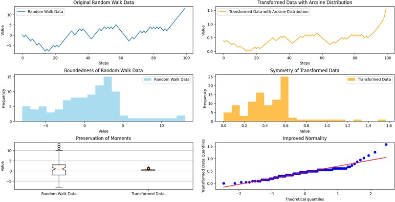
The Arcsine distribution is particularly adept at handling data constrained within specific bounds, making it an ideal choice for transforming random walk data. Mathematically, the transformation involves mapping the original bounded data to a new distribution defined over the entire real line. The Arcsine distribution accomplishes this by providing a smooth transition from the bounded interval $[a, b]$ to the entire real line.

The transformation process involves applying the inverse Arcsine function to the original random walk data. If $X$ follows a random walk, the transformed variable $Y$ follows an Arcsine distribution:

13

Y = a r c s i n (\frac{X - a}{b - a}) .

This transformation ensures that $Y$ now follows the Arcsine distribution, offering advantages in terms of symmetry and well-defined statistical properties.

The Arcsine distribution, being inherently symmetric, provides a powerful tool for mitigating the effects of non-normality in random walk data. The symmetry of the Arcsine distribution around its midpoint accommodates the deviations from normality, allowing for more robust statistical analyses.

The transformation preserves key statistical characteristics such as mean, variance, and higher moments, ensuring that important features of the original random walk data are retained in the transformed distribution. This preservation is crucial for maintaining the integrity of the underlying information during the transformation process.

In the realm of time series modeling, where random walk data is prevalent, the theoretical basis for using the Arcsine distribution lies in its ability to reconcile the bounded nature of the data with the assumptions and requirements of various statistical methods. The transformation enables the application of traditional statistical tools, originally designed for unbounded data, to random walk series with bounded intervals.

In the subsequent sections, we will delve into practical applications, showcasing how the theoretical foundations translate into actionable insights for data analysts and researchers seeking to extract meaningful information from random walk data.

3.3. Application in engineering

The application of the arcsine transformation in optics has been well-established for nearly a century. In optical engineering, when dealing with harmonically oscillating structures, the optical representation often involves describing the structure as a convolution of the static image and the point spread function. Remarkably, in the context of harmonic oscillations, the point spread function corresponds to the arcsine distribution.

This association arises due to the unique characteristics of the arcsine distribution, particularly its relevance in describing the diffraction patterns produced by optical systems in response to harmonic oscillations. As light interacts with oscillating structures, such as diffraction gratings or vibrating surfaces, it undergoes modulation and dispersion, resulting in a spread of intensity across the optical image. This spread, or blurring effect, is mathematically described by the arcsine distribution, which accounts for the probability distribution of light intensity across the image plane.

By understanding the optical system’s response in terms of the convolution of the static image and the arcsine distribution, engineers can effectively model and analyze the optical phenomena associated with harmonically oscillating structures. This knowledge is invaluable in various optical engineering applications, including image processing, microscopy, lithography, and sensor design, where precise control and understanding of light propagation and diffraction are essential for achieving desired performance and functionality.

The Arcsine Distribution Equation defines the probability density function (PDF) of the arcsine distribution is given by Eq. (1).

The Point Spread Function (PSF) in Optics describes the system’s response to light, represented as a convolution of the static image $I (x, y)$ and the arcsine distribution $A (x)$ :

14

P S F (x, y) = I (x, y) * A (x) .

The Diffraction Pattern Intensity is derived from the Fourier transform of the PSF, providing insight into the intensity distribution of diffraction patterns:

15

I_{d} (x) = {|F \{P S F (x, y)\}|}^{2} .

Additionally, the Modulation Function for Harmonic Oscillations characterizes the spatial variation of oscillating structures using a sinusoidal function:

16

M (x) = c o s (k x),

where $k$ is the wavevector associated with the oscillations.

Finally, the Optical Response Incorporating Modulation combines the modulation function with the PSF to yield the system’s response to harmonic oscillations:

17

O (x) = P S F (x) \cdot M (x) .

These equations provide a mathematical framework for understanding the optical behavior of harmonically oscillating structures and their representation using the arcsine transformation. By applying these equations, engineers can analyze diffraction phenomena, design optical systems, and optimize performance in various applications in optics and photonics.

3.4. Application in financial modeling

3.4.1. Introduction

The application of the Arcsine distribution in financial modeling proves to be particularly illuminating, especially when grappling with the inherent complexities of random walk data prevalent in stock prices and financial markets. This section unravels the intricacies of employing the Arcsine distribution as a transformative tool in the context of financial time series modeling.

Financial markets often exhibit behavior akin to random walks, with stock prices undergoing stochastic movements. The Arcsine distribution provides an elegant solution for modeling these price changes, offering a statistical foundation that aligns with the bounded nature of stock prices.

The transformation process involves mapping the original stock prices to the Arcsine distribution:

18

Y_{t} = a r c s i n (\frac{X_{t} - a}{b - a}),

where $X_{t}$ represents the stock price at time $t$ and $Y_{t}$ is the transformed variable following the Arcsine distribution. This transformation accommodates the upper and lower bounds, enhancing the applicability of traditional statistical models designed for unbounded distributions.

One of the critical aspects of financial modeling is the accurate representation of volatility. Random walks, inherent in financial time series, demonstrate diffusive behavior, leading to increasing variance over time. The Arcsine distribution facilitates a nuanced approach to capturing and modeling this volatility.

The variance in the transformed domain is given by:

19

V a r (Y_{t}) = \frac{1}{2} .

This constant variance aligns with the evolving nature of financial markets, making the Arcsine distribution a valuable tool for capturing the time-varying nature of volatility.

Risk management and option pricing heavily rely on understanding the distribution of potential outcomes. The Arcsine distribution, with its symmetric and bounded characteristics, proves beneficial in these domains. By transforming random walk data with the Arcsine distribution, analysts gain a more accurate representation of the risk associated with different market scenarios.

In the context of option pricing, where the underlying assumptions about the distribution of asset prices are crucial, the Arcsine distribution offers a flexible and robust framework. The transformed data aligns with the assumptions of certain option pricing models, enhancing the accuracy of pricing predictions.

The application of the arcsine distribution in financial modeling brings several benefits when analyzing random walk data. Firstly, it addresses the issue of asymmetry commonly found in such data, ensuring a more accurate representation of price movements and asset returns by achieving symmetry around its midpoint. Additionally, the distribution imposes bounds on the transformed data, confining it within a specified interval, which aligns well with the constraints often observed in financial markets. Furthermore, by utilizing the arcsine distribution, financial models can attain greater statistical robustness, leading to more reliable parameter estimation and improved predictive accuracy. Moreover, the distribution’s properties facilitate enhanced risk management by providing a clearer assessment of potential outcomes, enabling better decision-making and portfolio risk management. Lastly, the arcsine distribution aids in capturing volatility clustering phenomena inherent in random walk data, contributing to more precise volatility modeling and forecasting. In summary, leveraging the arcsine distribution in financial modeling offers significant advantages, including symmetry enhancement, boundedness, statistical robustness, improved risk management, and enhanced volatility modeling, ultimately assisting stakeholders in making informed decisions and managing market risk effectively.

3.4.2. Symmetry enhancement using the arcsine distribution

Symmetry enhancement using the arcsine distribution can improve modeling of price movements and asset returns with an example:

Consider a time series of daily returns for a stock, where negative returns are more frequent than positive returns, leading to a skewed distribution. This asymmetry in the data can make it challenging to accurately model the underlying dynamics of the stock’s price movements and forecast future returns.

Now, let’s apply the arcsine distribution transformation to the daily returns data. The arcsine transformation maps the original returns data onto the range [–1, 1], achieving symmetry around its midpoint. This means that both positive and negative returns are transformed to lie within the interval [–1, 1], effectively balancing out the asymmetry in the data.

For example, suppose we have the following daily returns data for a stock:

20

\{- 0.02, - 0.01, - 0.03,0.01, - 0.02,0.02,0.03, - 0.01, - 0.02,0.01\} .

After applying the arcsine transformation, the transformed returns data might look like this:

21

\{- 0.45, - 0.32, - 0.55,0.32, - 0.45,0.45,0.55, - 0.32, - 0.45,0.32\} .

Notice how the transformed data achieves symmetry around its midpoint (zero), with both positive and negative returns distributed more evenly across the range [–1, 1]. This symmetry enhancement can provide a more balanced and representative view of the stock’s price movements, enabling better modeling and analysis.

By achieving symmetry in the data, the arcsine distribution transformation helps mitigate the effects of skewness and improves the accuracy of statistical models used for forecasting future returns. This enhanced symmetry facilitates better understanding and interpretation of the underlying dynamics driving the stock’s price movements, ultimately leading to more informed investment decisions and risk management strategies.

3.4.3. Volatility modeling using the arcsine distribution

In this section, we delve into the process of volatility modeling using the arcsine distribution, focusing on a time series of daily returns for a financial asset like a stock or an index. Our objective is to effectively model the volatility inherent in these returns. We begin by preparing the data, followed by parameter estimation and volatility forecasting utilizing the arcsine distribution. Subsequently, we conduct back transformation to revert the forecasted volatility to its original scale, and finally, we evaluate the model’s performance. This comprehensive overview encapsulates the key stages involved in leveraging the arcsine distribution for volatility modeling.

In the initial stage, historical daily returns data for the financial asset is gathered. Utilizing this data, daily log returns are calculated using the formula $r_{t} = l n (\frac{P_{t}}{P_{t - 1}})$ , where $r_{t}$ represents the daily log return at time $t$ , and $P_{t}$ signifies the asset price at time $t$ . Subsequently, in the parameter estimation phase, the daily log returns are transformed into the range [–1, 1] via the arcsine transformation: $x_{t} = 2 \times a r c s i n (\sqrt{r_{t}})$ . Following this transformation, the mean and variance of the transformed data, $x_{t}$ , are estimated. Notably, the mean of the arcsine distribution is zero, with a known variance of 0.5 for the specified range. Moving to volatility forecasting, the estimated parameters of the arcsine distribution are leveraged to predict future volatility. One approach involves calculating the standard deviation of the transformed data ( $σ_{t} = \sqrt{0.5}$ ) as an estimate of volatility. Alternatively, more sophisticated methods like GARCH models can be employed for volatility forecasting based on the arcsine-transformed data. In the subsequent stage of back transformation, forecasted volatility derived from the arcsine-transformed data is converted back to the original scale using the inverse arcsine function: $r_{t} = {s i n}^{2} (x_{t} / 2)$ . Finally, the performance of the volatility model is evaluated using standard validation techniques such as out-of-sample testing and goodness-of-fit tests, and the forecasted volatility is compared with realized volatility to gauge the accuracy of the model.

By applying the arcsine distribution to model volatility, we can capture the underlying characteristics of the data while ensuring symmetry and boundedness, leading to more accurate and robust volatility forecasts. This approach provides a valuable tool for risk management and decision-making in financial markets.

3.4.4. Value-at-Risk (VaR) estimation using the arcsine distribution

In this section, we outline the steps in a financial risk analysis, covering data preparation, parameter estimation, VaR computation, result interpretation, and validation.

In the data preparation phase, historical daily returns data for a financial asset is collected. Utilizing this data, daily log returns are computed using the formula $r_{t} = l n (\frac{P_{t}}{P_{t - 1}})$ , where $r_{t}$ denotes the daily log return at time $t$ , and $P_{t}$ represents the asset price at time $t$ . Subsequently, in the parameter estimation step, the daily log returns are transformed into the range [–1, 1] through the arcsine transformation: $x_{t} = 2 \times a r c s i n (\sqrt{r_{t}})$ . Mean and variance estimation of the transformed data, $x_{t}$ , follows, noting that the mean of the arcsine distribution is zero, and the variance is $0.5$ for the specified range. Proceeding to VaR calculation, once the parameters of the arcsine distribution are estimated, VaR is computed at a specified confidence level. For instance, to derive VaR at the 95 % confidence level, the critical value $z$ such that $P (X \leq z) = 0.95$ is determined, where $X$ follows the arcsine distribution. Employing the inverse arcsine function, $z$ is found, and subsequently back-transformed to obtain $r_{V a R}$ , representing the VaR threshold in the original scale. In the interpretation phase, VaR signifies the maximum potential loss of a portfolio at the specified confidence level over a given time horizon. For instance, a VaR of 5 % at the 95 % confidence level implies a 5 % chance of the portfolio incurring losses exceeding the VaR threshold within the designated time frame. Finally, the validity of VaR estimates is assessed through historical backtesting and stress testing techniques in the validation and sensitivity analysis stage, which evaluates the impact of variations in model parameters, such as confidence level and time horizon, on VaR estimates.

By applying the arcsine distribution to estimate VaR, we can obtain robust and reliable risk measures that account for the underlying characteristics of the data, such as symmetry and boundedness. This approach provides a valuable tool for risk management and decision-making in financial markets, helping investors and financial institutions quantify and manage market risk effectively.

4. Conclusions

In the evolving landscape of statistical modeling, the Arcsine distribution stands as a testament to the importance of considering the specific characteristics of the data at hand. Its simplicity, adaptability, and theoretical soundness position it as a valuable asset for statisticians, researchers, and analysts seeking to unlock insights from a variety of datasets.

As we continue to push the boundaries of statistical methodologies, the Arcsine distribution serves as a reminder of the rich and varied toolkit available to researchers. Its applications, both established and emerging, contribute to the broader landscape of probability distributions, offering a nuanced and effective approach to transforming and analyzing data.

The novelty of our study lies in its interdisciplinary approach that bridges the gap between statistical methodology and engineering applications, particularly in the analysis of random walk data. By leveraging the arcsine distribution, a statistical tool traditionally used in probability theory and mathematical statistics, the article introduces a novel framework for analyzing and interpreting random.

References

K. Nikodem, “On convex stochastic processes,” Aequationes Mathematicae, Vol. 20, pp. 184–197, 1980.

Publisher
C. H. Papadimitriou, P. Raghavan, H. Tamaki, and S. Vempala, “Latent semantic indexing: A probabilistic analysis,” Journal of Computer and System Sciences, Vol. 61, No. 2, pp. 217–235, 2000.

Publisher
J. B. Kadane and D. A. Schum, “A probabilistic analysis of the Sacco and Vanzetti evidence,” in Wiley Series in Probability and Statistics, Vol. 40, Wiley, 1997, https://doi.org/10.1002/9781118150580

Publisher
M. Graczyk, T. Moan, and O. Rognebakke, “Probabilistic analysis of characteristic pressure for lng tanks,” Journal of Offshore Mechanics and Arctic Engineering-Transactions, Vol. 128, 2006.

Publisher
S. Karlin and J. Mcgregor, “Random walks,” Illinois Journal of Mathematics, Vol. 3, No. 1, pp. 66–81, 1959.

Publisher
G. Weiss and R. Rubin, “Random walks: theory and selected applications,” in Advances in Chemical Physics, Vol. 52, John Wiley & Sons, Ltd, 2007, pp. 363–505.

Publisher
E. Scalas, “The application of continuous-time random walks in finance and economics,” Physica A: Statistical Mechanics and its Applications, Vol. 362, pp. 225–239, 2006.

Publisher
R. Chattamvelli and R. Shanmugam, Arcsine Distribution. Cham: Springer International Publishing, 2021, pp. 57–68.

Publisher
R. Mantovani, F. Folla, G. Pigozzi, S. Tsuruta, and C. Sartori, “Genetics of lifetime reproductive performance in Italian heavy draught horse mares,” Animals, Vol. 10, p. 1085, Jun. 2020.

Publisher
D. Grahn and K. F. Hamilton, “Genetic variation in the acute lethal response of four inbred mouse strains to whole body x-irradiation,” Genetics, Vol. 42, No. 3, p. 189, 1957.

Publisher
Y. L. Tung, Z. Ahmad, and E. Mahmoudi, “The arcsine-x family of distributions with applications to financial sciences,” Computer Systems Science and Engineering, Vol. 39, pp. 351–363, Jan. 2021.

Publisher
B. C. Arnold and R. A. Groeneveld, “Some properties of the arcsine distribution,” Journal of the American Statistical Association, Vol. 75, No. 369, pp. 173–175, 1980.

Publisher
G. Aryal, “Transmuted log-logistic distribution,” Journal of Statistics Applications and Probability, Vol. 2, pp. 11–20, Mar. 2013.

Publisher
G. Cordeiro, A. Lemonte, and A. Campelo, “Extended arcsine distribution to proportional data: Properties and applications,” Studia Scientiarum Mathematicarum Hungarica, Vol. 53, pp. 440–466, Dec. 2016.

Publisher
S. Bleed and A. Abdelali, “Transmuted arcsine distribution properties and application,” International Journal of Research – GRANTHAALAYAH, Vol. 6, pp. 38–47, Oct. 2018.

Publisher
W. T. Shaw and I. R. C. Buckley, “The alchemy of probability distributions: Beyond gram-charlier and cornish-fisher expansions, and skew-normal or kurtotic-normal distributions,” arXiv:0901.0434, Feb. 2007.

Search CrossRef
J. Masel, “Genetic drift,” Current Biology, Vol. 21, No. 20, pp. R837–R838, 2011.

Publisher
R. Gallotti, R. Louf, J.-M. Luck, and M. Barthelemy, “Tracking random walks,” Journal of The Royal Society Interface, Vol. 15, No. 139, p. 20170776, 2018.

Publisher
E. Viola, O. Weinstein, and H. Yu, “How to store a random walk,” in Proceedings of the Fourteenth Annual ACM-SIAM Symposium on Discrete Algorithms, pp. 426–445, 2020.

Publisher

About this article

Received

19 March 2024

Accepted

19 April 2024

Published

23 May 2024

DOI

https://doi.org/10.21595/mme.2024.24105

Keywords

random walks

arcsine distribution

statistical transformation

Acknowledgements

The authors have not disclosed any funding.

Data Availability

The datasets generated during and/or analyzed during the current study are available from the corresponding author on reasonable request.

Author Contributions

Yassine Laarichi: project administration, conceptualization, software,methodology, writing – original draft preparation, supervision. Mariem Elkaf: data curation, resources, validation, writing – original draft preparation. Amal Aloui: formal analysis, writing – review and editing, validation. Oualid Rholam: investigation, writing – review and editing, validation

Conflict of interest

The authors declare that they have no conflict of interest.

This is an open access article distributed under the Creative Commons Attribution License, which permits unrestricted use, distribution, and reproduction in any medium, provided the original work is properly cited.

Research article

2020 09 30

Fault severity assessment of rolling bearings method based on improved VMD and LSTM

Zhihua Liang, Jiangtao Cao, Xiaofei Ji, Peng Wei

Research article

2017 05 30

Experimental HALTs with sine-on-random synthesized profiles

Marco Troncossi, Alessandro Rivola

Research article

2016 11 15

A hybrid approach of symbolic aggregate approximation and bitmap: application to fault diagnosis of reciprocating compressor valve

Lixiang Duan, Yulong Zhang, Xuduo Wang, Jinjiang Wang

Research article

2016 11 15

A hybrid artificial neural network with Dempster-Shafer theory for automated bearing fault diagnosis

Kar Hoou Hui, Ching Sheng Ooi, Meng Hee Lim, Mohd Salman Leong

Y. Laarichi, M. Elkaf, A. Aloui, and O. Rholam, “Transforming data with the arcsine distribution for random walks,” Mathematical Models in Engineering, Vol. 10, No. 2, –10, May 2024, https://doi.org/10.21595/mme.2024.24105

Copy Extrica

Copied to clipboard!

TY  - JOUR
DO  - 10.21595/mme.2024.24105
UR  - https://doi.org/10.21595/mme.2024.24105
TI  - Transforming data with the arcsine distribution for random walks
T2  - Mathematical Models in Engineering
AU  - Laarichi, Yassine
AU  - Elkaf, Mariem
AU  - Aloui, Amal
AU  - Rholam, Oualid
PY  - 2024
DA  - 2024/05/23
PB  - Extrica
VL  - 10
IS  - 2
SN  - 2351-5279
SN  - 2424-4627
ER  - 

Copy Ris

Copied to clipboard!

 @article{Laarichi_2024, title={Transforming data with the arcsine distribution for random walks}, ISSN={2424-4627}, url={https://doi.org/10.21595/mme.2024.24105}, DOI={10.21595/mme.2024.24105}, journal={Mathematical Models in Engineering}, publisher={JVE International Ltd.}, author={Laarichi, Yassine and Elkaf, Mariem and Aloui, Amal and Rholam, Oualid}, year={2024}, month=may }

Copy Bibtex

Copied to clipboard!

[1]Y. Laarichi, M. Elkaf, A. Aloui, and O. Rholam, “Transforming data with the arcsine distribution for random walks,” Mathematical Models in Engineering, May 2024, doi: 10.21595/mme.2024.24105.

Copy IEEE

Copied to clipboard!

Laarichi, Yassine, Mariem Elkaf, Amal Aloui, and Oualid Rholam. “Transforming Data with the Arcsine Distribution for Random Walks.” Mathematical Models in Engineering, May 23, 2024. https://doi.org/10.21595/mme.2024.24105.

Copy Chicago

Copied to clipboard!

Transforming data with the arcsine distribution for random walks

Abstract

1. Introduction

2. Understanding random walks

2.1. Challenges in analyzing random walks

3. Main results

3.1. Introduction to the arcsine distribution

3.2. Theoretical basis for transformation

3.3. Application in engineering

3.4. Application in financial modeling

3.4.1. Introduction

3.4.2. Symmetry enhancement using the arcsine distribution

3.4.3. Volatility modeling using the arcsine distribution

3.4.4. Value-at-Risk (VaR) estimation using the arcsine distribution

4. Conclusions

References

About this article

Related Articles