Abstract
In order to solve the problem of selection of appropriate wavelet basis function and clearly show the physical meaning of Empirical Mode Decomposition (EMD), an improved Variational Mode Decomposition (VMD) method with Long Short-Term Memory (LSTM) neural network is proposed. With the Cuckoo Search (CS) algorithm, the central frequency updating rules of VMD are optimized. And the low efficiency and local optimum problem is avoided. Meanwhile the decomposition layer number is found by the instantaneous frequency theory. For improving the prediction accuracy in traditional regression prediction methods, a LSTM neural network is designed for regression prediction of time sequence characteristics. The proposed method is implemented on actual bearings data which is derived from the bearing laboratory of Case West Reserve University in the United States and the University of Cincinnati Bearing Data Center. The experimental results showed that the improved VMD method was more robust and more accurate than the other traditional methods. And it has some practical value for real application and guiding significance for theory.
Highlights
- Raised the CS-VMD and instantaneous frequency theory to solve the shortcomings of VMD theory.
- Using LSTM to solve the problem of bearing performance evaluation as the first time.
- Found two shortcomings of the VMD algorithm.
1. Introduction
As a precision component, rolling bearings are widely used in rotating machinery. Because of the natural working conditions, the rolling bearings are particularly vulnerable. According to the research, about 30 % of the rotating machinery faults were caused directly or indirectly by the faults of rolling bearings, which brought huge economic and life losses [1, 2]. So, the performance assessment of rolling bearings and its maintenance according to its situation are the most important works to ensure the safe, stable, efficient and accurate operation of rotating machinery. It is also one of the most popular subjects of research in the academic and industrial area [3].
In general, the performance assessment of rolling bearings is divided into three parts: signal preprocessing, features extraction and regression prediction. The main purpose of signal preprocessing is to eliminate noise. Traditional methods include Fourier Transform (FT), Wavelet Transform (WT) and Empirical Mode Decomposition (EMD), etc. [4]. However, many shortcomings have been found in these traditional methods. In recent years, some methods based on WT were developed. Hou, Zhiqiang, et al. developed a new multi-speed fault diagnostic approach which was presented by using self-adaptive wavelet transform components generated from bearings vibration signals [5]. Yongbo Li, et al. developed a method based on Tunable Q-factor Wavelet Transform (TQWT) to analyze early fault diagnosis [6]. Although the above methods achieved some better performance, the shortcomings of insufficient wavelet decomposition adaptive performance still exist. EMD is a method which can self-adaptive decompose wavelet transform functions, and many improved methods were built. Zhaohua Wu, et al. proposed an improved EMD method named as the Ensemble Empirical Mode Decomposition (EEMD), by adding a finite amount of Gaussian noise into the signal, and decomposed it with EMD [7]. Although the EEMD can eliminate the Modal Mixing of EMD, EEMD still has the problem to clearly explain the physical meaning. Jonathan S. Smith proposed the Local Mean Decomposition (LMD), and used it to analyze EEG perception data [8]. Although each component decomposed by LMD has practical physical meaning, the sampling frequency, sliding span selection and endpoint effects will affect the accuracy. Dragomiretskiy K. et al. proposed a new signal processing method named as the Variational Mode Decomposition (VMD) [9]. VMD used the Non-recursive decomposition and alternating direction method of multipliers (ADMM) to solve the optimal value of the center frequency and bandwidth of each modal component. VMD has a strong adaptability, a clearly physical meaning and a strong robustness. Wang Y. et al. compared the EMD, EEMD, VMD and other methods, and verified that the VMD has better effects and no modal mixing [10]. Although the VMD has been well used in fault diagnosis of rolling bearings, metal defect diagnosis and speech signal processing, it also has two disadvantages. One is that the central frequency falls into local optimum, and the other is the problem of selection of the number of decomposition layers. It still has further way to go.
Traditional methods of regression prediction include K-nearest neighbor (KNN), artificial neural network (ANN), and support vector regression (SVR), etc. Min-Ling Zhang, et al. used the multi-label KNN to analyze yeast gene, natural scene classification and automatic web page categorization [11], but the calculation of KNN is very complicated. Li et al. presented an integration method of artificial neural network and empirical mode decomposition to identify fault severity in rolling bearings, and the results demonstrated that the integration method had been successful in machine fault severity diagnosis [12], but it had been hard to obtain so lots of data to support the training of ANN. Elish et al. investigated and empirically evaluated and compared multi-layer perceptron (MLP), radial basis function (RBF), KNN and SVR, etc. and found that the SVR was more accurate in predicting fault density [13]. Patel et al. compared SVR with ANN and proved that SVR was better than ANN in regression prediction [14]. Although SVR is better than KNN and ANN in regression prediction, the selection of parameters in SVR has a great influence on the accuracy. These traditional regression prediction methods have certain effects on the processing of non-timing signals. However, they cannot preserve the timing correlation of signals; the processing of timing signals is slightly insufficient.
Fig. 1Rolling bearings performance evaluation flow chart

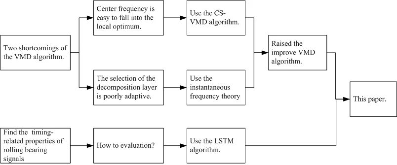
In this paper, an assessment of rolling bearings performance based on improved VMD and Long Short-Term Memory (LSTM) has been presented. By optimizing the VMD with the Cuckoo Search (CS) algorithm, the center frequency can be prevented from falling into local optimum, and the number of decomposition layers can be determined by the instantaneous frequency theory. So the signal noise can be effectively reduced. As shown in Fig. 1, the flow chart of the performance assessment of rolling bearings is designed. Section 2 presents the processing and features extraction of bearings vibration signal. Section 3 presents the prediction method for rolling bearings life. The experiment research is given in Section 4. The conclusion is drawn in Section 5.
Note: The frequency units are Hz, the amplitude/var/rms/kurtosis units are mm and the data units are group except for special instructions in this paper.
2. Processing and features extraction of bearings vibration signal
2.1. Variational mode decomposition
VMD is a new adaptive time-frequency analysis method with a clear physical meaning [10]. It is an iterative solution process for a special variational model, and includes Wiener Filtering, Hilbert Transform, analytical signal, frequency mixing and heterodyne demodulation concepts.
VMD abandons the definition of the intrinsic mode function (IMF) in the EMD theory and redefines the IMF as shown in Eq. (1):
where is the th component of IMF, and are the instantaneous amplitude and instantaneous phase of . The function is a non-reducing function, so the instantaneous frequency . Since and vary much slower than , it can be assumed that is a harmonic signal with constant amplitude and frequency during a short time.
On the basis of the above, the VMD theory assumes that the input signal is composed of IMFs with limited bandwidth and different center frequencies. The constraint is that the sum of the individual IMFs is equal to the input signal , and the variational model of the signal decomposition is constructed with the minimum sum of the estimated bandwidths of each IMF. The specific process is as follows:
(1) Hilbert Transform. Hilbert Transform for each IMF is applied to obtain a single-side spectrum of :
(2) Frequency mixing. Mixing a pre-estimated center frequency for each IMF, and each IMF spectrum is moved to the baseband:
(3) Bandwidth estimation. The value is calculated by Eq. (3), and the bandwidth is estimated for each IMF.
(4) Constraints are introduced to establish an optimization model:
where is the number of IMF, , is the center frequency of .
In order to solve the above variational model, the quadratic penalty factor and the Lagrange operator are introduced, and the augmented Lagrange function is established in Eq. (5):
where is the penalty factor, and it can guarantee the accuracy of signal under Gaussian noise. is the Lagrange operator, and it can ensure the strictness of the model. Using alternating direction method of multipliers (ADMM) to update , and , and to search the saddle point of Lagrange function. is decomposed into IMFs:
It is converted to the frequency domain by Parseval/Plancherel Fourier Transform in Eq. (7):
The variable substitution is performed by , and then converted into a non-negative frequency domain. Finally, the updated expression of is obtained as follows:
Similarly, the update expression of can be obtained as follows:
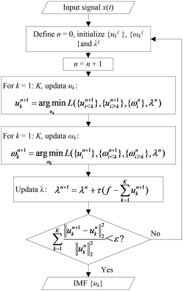
The solution process of the variational model is shown in Fig. 2. The initialization values of , , are 0.
2.2. VMD based on Cuckoo search algorithm
2.2.1. Cuckoo search algorithm
Cuckoo Search was a self-heuristic algorithm developed by Xin-She Yang and Suash Deb in 2009 based on the parasitic brooding behavior of cuckoos [15]. By adding Levy flight to enhance the global search ability, Cuckoo Search successfully avoids falling into local optimum.
Levy flight is a random walk pattern with a step-length distribution that is heavytailed [15]. In this model, short-distance exploration and occasional long-distance walking can increase the population diversity and avoid falling into the local optimum. Generating random numbers with Levy flight include two steps: selection of random directions and generation of step sizes subject to Levy distribution. In the Mantegna algorithm, the step size can be calculated using the following variables and which obey the Gaussian distribution:
where the variance can be calculated using Eq. (11):
Fig. 2VMD flow chart
CS is a more efficient algorithm based on the brooding behavior of the cuckoo and the Levy flight. The algorithm uses a balanced combination of local random walks controlled by the switch parameter and global exploration random walks.
The local random walk is as shown in Eq. (12):
where represents dot product, is a unit step function, is a uniformly distributed random number, is a step size scaling factor, is a switching parameter, is a step size, , are two random different solutions.
Global exploration of random walks using Levy flight:
where is the step size scaling factor, is the step size, and is a constant for a specific . Through the combination of local random walks and global exploration random walks, CS can effectively solve the problem of local optimum.
2.2.2. CS-VMD algorithm
CS-VMD algorithm uses the CS algorithm to find the optimal of the VMD, and then finds the optimal and .
The local random walk is as shown in Eq. (15):
where represents dot product, is a unit step function, is a uniformly distributed random number, is a step size scaling factor, is a switching parameter, is a step size, , are two random different solutions.
Global exploration of random walks using Levy flight:
where is the step size scaling factor, is the step size, and is a constant for a specific .
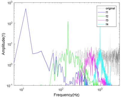
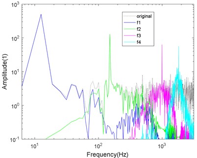
CS-VMD algorithm can effectively solve the problem that the center frequency of VMD falls into local optimum. For clearly showing the performance of CS-VMD, a signal function is tested as shown in Eq. (17), and the comparison results by VMD and CS-VMD are shown in Fig. 3:
where 2, 24, 288, 158 and is a random noise.
Fig. 3Logarithmic spectrum of signals processed by a) VMD and b) CS-VMD
a)
b)
As shown in Fig. 3, the signal center frequencies processed by VMD tend to fall into local optimum, and modal mixing has occurred. Then it is difficult to accurately remove the noise. However, the CS-VMD avoids falling into local optimum, the spectrum separation is more accurate, and the ability to remove noise is stronger.
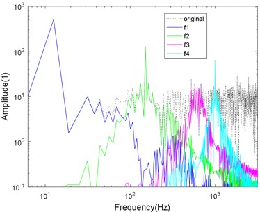
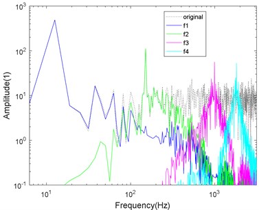
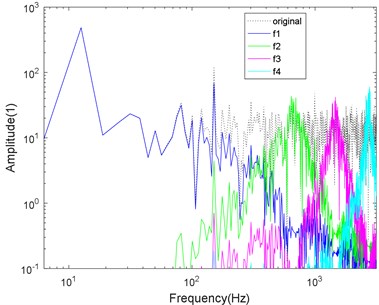
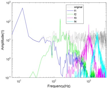
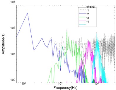
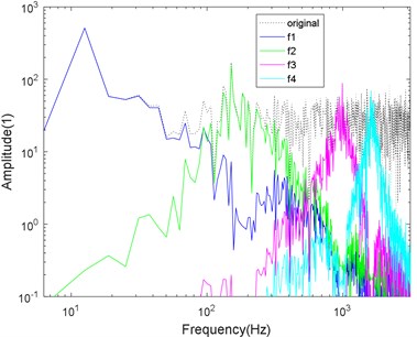
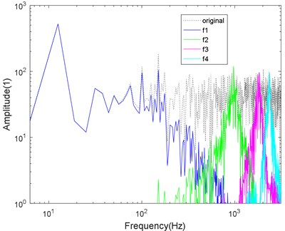
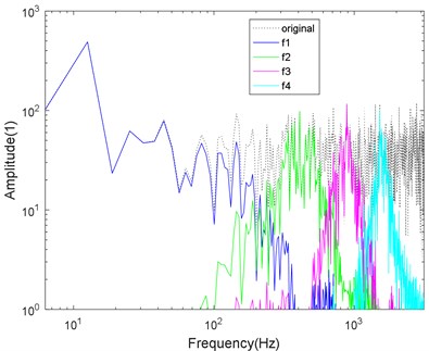
In order to test the ability to remove the noise, Eqs. (18-21) are the same one but with different SNR, and the comparison results by VMD and CS-VMD are shown in Figs. 4-7:
where 2, 24, 288, 158 and is a random noise.
Fig. 4Logarithmic spectrum of signals processed by a) VMD and b) CS-VMD in low noise
a)
b)
Fig. 5Logarithmic spectrum of signals processed by a) VMD and b) CS-VMD in moderate noise
a)
b)
Fig. 6Logarithmic spectrum of signals processed by a) VMD and b) CS-VMD in strong noise
a)
b)
Fig. 7Logarithmic spectrum of signals processed by a) VMD and b) CS-VMD in super-strong noise
a)
b)
As shown in Figs. 4-7, the mode aliasing occurs in VMD under the interference of any intensity noise. CS-VMD performs well under moderate and low noise as shown in Figs. 4-5. Even under the strong noise, CS-VMD can still accurately find the center frequency as shown in Fig. 6. When the noise significantly exceeds the original signal, the performance of CS-VMD begins to decline, but it is still stronger than VMD as shown in Fig. 7.
2.2.3. Selection problem for layer number
The number of decomposition layers will directly affect the performance. Once the number is small, the decomposed modal components will lose information or modal aliasing will occur. If the number is large, the excessive decomposition will occur. Therefore, Chen Dongning, et al. analyzed the data of the bearing laboratory of the Case Western Reserve University in the United States [17]. They selected the number of decomposition layers = 2-6 for VMD decomposition, and determined the value by observing the center frequency of each modal component, as shown in Table 1.
Table 1Center frequency corresponding to different K
Decomposition layers | Center frequency (Hz) | ||||
2 | 2646 | 3499 | – | – | – |
3 | 1381 | 2715 | 3509 | – | – |
4 | 505 | 1328 | 2713 | 3507 | – |
5 | 503 | 1336 | 2692 | 3470 | 3510 |
6 | 455 | 1232 | 2681 | 3304 | 3562 |
The method considers that when ≥ 5, an excessive decomposition occurs, so = 4 is taken.
In this paper, we studied VMD thoroughly and found that if there were too many decomposition layers, the components would be discontinuous, especially in the case of high-frequency components. Even though it is a high-frequency component, the average instantaneous frequency will be lower. Therefore, a method based on the mean value of instantaneous frequency is proposed to determine the number of decomposition layers. The testing data is derived from the bearing laboratory of the Case Western Reserve University in the United States. The Bearing Laboratory Platform of Case Western Reserve University in the USA includes motor, torque sensor, power meter and electronic control equipment. The bearing supporting motor is tested. The pitting fault is simulated on the bearing by the EDM technology. The fault diameter is 0.18 mm, 0.36 mm, 0.53 mm and 0.71 mm respectively, and the fault is simulated from weak to serious, when the sampling frequency is 12000 Hz. The decomposition layer number = 2-7 is selected for VMD decomposition, and the mean value of the instantaneous frequency is calculated for each layer decomposition. The mean value of the instantaneous frequency can be calculated by Eq. (22):
where is the instantaneous frequency mean value of the th layer ( 1, 2, …, ), is the number of sampling points of each layer component, is the instantaneous frequency of the th sampling point of the th layer. The first derivative of the instantaneous phase is defined as the instantaneous frequency, which is usually calculated by the Hilbert transform. The calculation method is introduced below the Eq. (1). is taken as the horizontal axis and is taken as the vertical axis, as shown in Fig. 8.
Fig. 8Instantaneous frequency mean curve at different K values
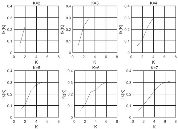
It can be seen from Fig. 8 that the slope of the curve from = 4 to = 5 is much lower than before.
When = 2, the slope of the curve is very large. When = 3, the slope of the curve between = 2 and = 3 decreases slightly. When = 4, the slope of the curve from = 3 to = 4 is not significantly reduced compared to = 3. However, when = 5, the slope of the curve is significantly reduced. When = 6, the slope of the curve is not significantly reduced compared to = 5. When = 7, the slope of the curve is not significantly reduced compared to = 6.
So when = 5, the curve slope is significantly reduced, the phenomenon of excessive decomposition causes decreasing the instantaneous frequency, so = 4 is a reasonable number of decomposition layers. The use of this method can solve the problem of the number of decomposition layers of the VMD.
2.3. Features extraction
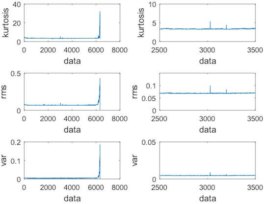
The kurtosis, root mean square, and variance features of the rolling bearings signal are extracted and compared as shown in Fig. 9.
The results in Fig. 9 show the kurtosis, root mean square, and variance as features to display the time sequence spectrum. The right side is the partially enlarged image of the left image. It can be found that there are obvious peaks in the vicinity of the 3000th series of time sequence data. It means that the original signal of the data set has large noise interference, but the variance feature is less interfered. Then the variance is selected as the feature for life prediction research of rolling bearings.
Fig. 9Comparison of different features of signal
3. Prediction method for rolling bearings life
Currently used rolling bearing life prediction methods include KNN, ANN, and SVR, etc. Since the state of these conventional regression methods is only related to the previous moment, the regression effect on the timing signals is poor. LSTM can relate the state of a certain moment to the state of a previous moment, and has been widely used in the field of speech recognition [18]. Considering that the rolling bearings vibration signal and the speech signal are both time-dependent one-dimensional signals, the LSTM is used for the prediction of rolling bearings life in this paper.
3.1. Long short-term memory
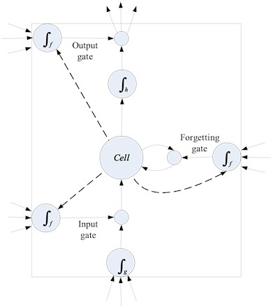
LSTM is an improved Recurrent Neural Network (RNN) which can efficiently process time sequence signals. LSTM is established by adding long and short-term memory cells to the hidden layer of RNN. It consists of a set of structures called as Cells. A Cell structure consists of three gate elements: input gate, forgetting gate, and output gate. After a data is inputted into the network of the LSTM, it is assessed according to the rules whether the data is useful, the data conforming to the algorithm authentication is left, and the data that is inconsistent is forgotten by the forgetting gate. Moreover, the structure can achieve a constant error flow through a constant error conveyor belt, thereby solving the problem of gradient disappearance [19]. The long and short-term memory cell structure of LSTM is shown in Fig. 10 [20].
Due to the introduction of long and short-term memory cells, LSTM has good memory capabilities. Its gate activation function is generally a sigmoid function (as shown in Eq. (23)), and its range is (0, 1). Input gate, forgetting gate, and output gate are multiplied by a state value. When the gate output is 0, multiplication with any state will be 0, which can discard unwanted information. When the gate output is 1, the multiplication with any state will not change, so that all the neuron information can be retained. Therefore, the LSTM selectively retains information based on state values, resulting in higher prediction accuracy:
Fig. 10Long and short-term memory cell structure of LSTM
3.2. Forward transfer algorithm of LSTM
In the phase of forward transfer, the input received by the Cell structure of LSTM at time includes both the input of the neural network at that time, and the output of the hidden layer at the previous moment.
In the first step, LSTM selects the discarded information through the forgetting gate, and the hidden state at the time and at the input time are used as the input of the forgetting gate. After the activation function is processed, the output of the forgetting gate is obtained by Eq. (24):
where is the weight of forgotten gate, is the offset, is the sigmoid activation function.
In the second step, the LSTM will select the information that needs to be saved in the neuron. This step is implemented through the input gate. Calculation process includes two parts. The first part uses the sigmoid activation function to determine the value that needs to be updated in Eq. (25). The second part uses the tanh function to generate a new candidate vector in Eq. (26). The both parts are multiplied to update the state of the cell:
where and are the corresponding weights respectively, and are the corresponding offsets respectively, and is the sigmoid activation function.
The Cell status update also includes two parts: One part is the output product of the forgetting gate and the cell output at time , and the other part is the output product of the input gate and the candidate vector . As shown in Eq. (27):
the status of the output gate is finally updated, and the input of output gate is related to the current state of Cell. Firstly, the state of Cell at time is processed by the sigmoid activation function to obtain a partial output, and then the state of Cell at time is processed by the tanh function. The product of the two is used as the final output result as shown in Eq. (28) and (29):
where is the output gate weight, is the state of the cell at time , is the offset of the output gate, and is the sigmoid activation function.
3.3. Back propagation algorithm of LSTM
In the phase of back propagation, LSTM uses a time-based back propagation algorithm (BPTT). After inputting the training samples, the forward-transfer process obtains the output of the neural network at time . By calculating the output error, the gradient is calculated layer-by-layer from . The specific steps of the BPTT algorithm of LSTM are as follows:
(1) The output of each neuron and the output of the input gate, forgetting gate, output gate, and Cell in the LSTM module are forward calculated.
(2) Reverse calculation of the output error for each neuron. Starting from the current time , the errors of each time are calculated one-by-one, and the errors are propagated to the upper layer. The error is the partial derivative of the weighted input of the error function to the neuron .
(3) Gradient calculation of each weight based on the corresponding error.
(4) Iterative update of the weights using the stochastic gradient descent.
About the calculation part of the gradient, the key to the LSTM algorithm is to calculate the gradient of the Cell, including the calculation of partial derivatives for input gate, forgetting gate, and output gate as shown in Eq. (30):
where is the error gradient of the Cell output at time , is the gradient of the current Cell output, is the gradient of the output gate, is the gradient of the Cell at the next moment, is the gradient of the forgetting gate, and is the gradient of the input gate.
4. Experiment and experiment results
4.1. Experiment preparation
The failure data of the rolling bearings used in this experiment is derived from the bearing laboratory of the Case West Reserve University in the United States and the University of Cincinnati Bearing Data Center.
The test rig consists of four bearings mounted on one shaft, as shown in Fig. 11. There are three data sets. Each bearing of data set 1 has two accelerometers (-axis and -axis), and each bearing of data set 2 and data set 3 has one accelerometer. The sensor position is also shown in Fig. 11. Each data set represents bearing life data from the start of a new bearing until the bearing is completely damaged. In this paper, the data set 3 has been used. The sampling frequency is 20 kHz, recorded every 10 minutes, and each time recording 1 second vibration signal, 20480×4 data in a total of 6324 sets of data.
Fig. 11Bearing test rig and sensor placement illustration
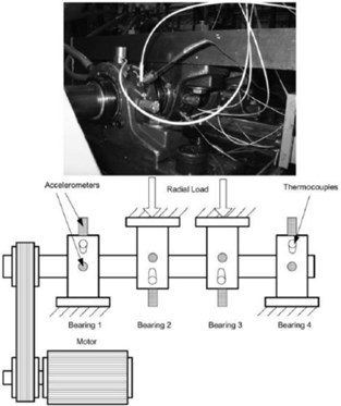
The normal bearing signal is shown in Fig. 12, the signal of slight bearing fault is shown in Fig. 13, the signal of medium bearing fault is shown in Fig. 14, and the signal of serious bearing fault is shown in Fig. 15.
Fig. 12Normal bearing signal
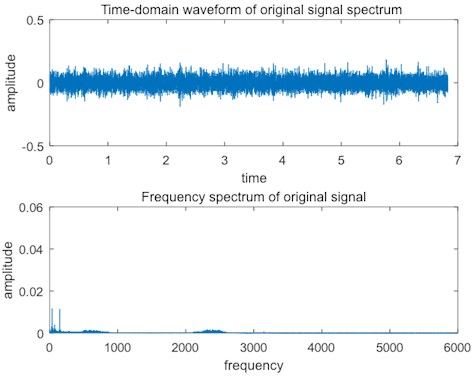
As shown in Fig. 12, the normal bearing signal has weak amplitude in the time domain spectrum, and only the low frequency part has obvious impulses in the frequency spectrum, which are the natural frequency and frequency multiplication of the bearings.
As shown in Fig. 13, when a slight fault occurs in bearings, the amplitude of the time domain spectrum increases slightly, and the frequency spectrum shows more obvious impulses of the mid-frequency band, which indicates that the defect of the bearings is not serious, so the vibration frequency is generated in the mid-frequency band.
As shown in Fig. 14, when the medium fault occurs in the bearings, the amplitude of the time domain spectrum increases obviously, the impulses of the mid-frequency in the frequency-domain spectrum are more obvious, and the impulses of the high-frequency band are obvious, which indicates that the bearing defect is serious.
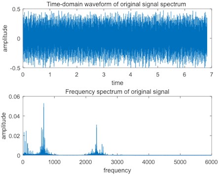
As shown in Fig. 15, when a serious fault occurs in the bearings, the amplitude of the time domain spectrum increases strongly, and the impulses of the middle and high frequency bands of the frequency-domain spectrum are particularly obvious. At this time, the bearings cannot work properly and needs to be shut down and maintained as soon as possible.
Fig. 13Slight bearing fault signal
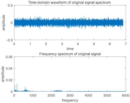
Fig. 14Medium bearing fault signal
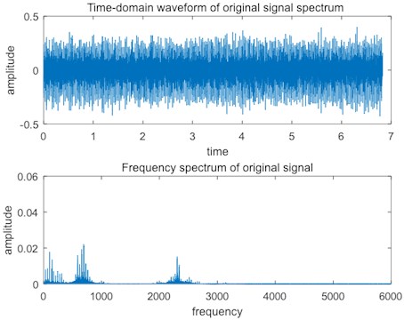
Fig. 15Serious bearing fault signal
4.2. Experimental result
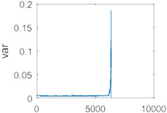
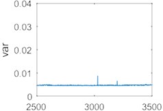
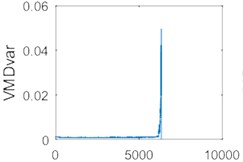
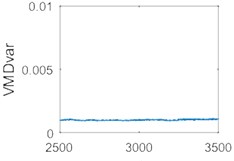
The data was processed using the improved VMD, and the variance of each group of data was extracted as a feature and compared with variance feature of the original data as shown in Fig. 16.
Fig. 16Comparison of variances of each data group before and after using improved VMD
a)
b)
c)
d)
Fig. 16(a) and Fig. 16(b) demonstrate the variance features sequence of the original data. Fig. 16(c) and Fig. 16(d) show the variance features sequence of the data using the improved VMD. Fig. 16(b) and 16(d) are local enlargements of Fig. 16(a) and 16(d), respectively. As it can be seen from Fig. 16, the signal that is not processed by the improved VMD is shown in Fig. 16(b), and there is a significant fluctuation in the vicinity of the 3000th data group because of the large noise interference of the data (It may be caused by sudden changes in working state or impulse noise). Signals are processed using the improved VMD in Fig. 16(d), no significant fluctuations occurs, and the variance is also reduced after the signal has been processed by the improved VMD. Therefore, using the improved VMD to process the data and extract the variance as a feature can effectively reduce the influence of noise, and provide a guarantee for a further signal analysis.
Vector regression is supported based on the particle swarm optimization (PSO-SVR) and LSTM regression prediction for the obtained feature sequence, and the results are shown in Fig. 17 and Fig. 18.
As shown in Figs. 17-20, there are some errors between PSO-SVR regression / ANN regression / KNN regression and real signal, and the regression signal also shows some fluctuations, which indicate that the regression effects are PSO-SVR > ANN > KNN. However, LSTM regression has a higher degree of fitting with the real signal, and the regression is stable, so LSTM regression is better than any others. Table 2 compares the absolute total errors between the regression methods.
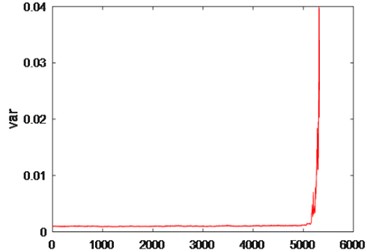
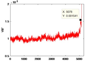
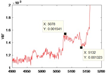
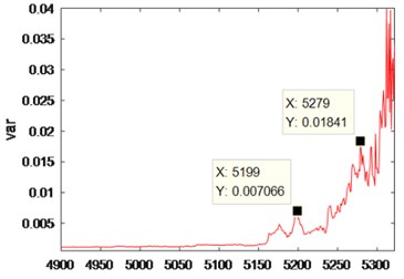
The regression data was analyzed (Fig. 21), where in Fig. 21(a) is an overall graph of regression data, and Fig. 21(b), 21(c), and 21(d) are local enlargements of Fig. 21(a).
It can be seen from Fig. 21 that after denoising by the improved VMD, the Spectrum of Time Series of Variance has a significant rise in the vicinity of the 5078 data, and the rolling bearing has a slight failure. After a significant drop (vicinity of 5132), the Spectrum of Time Series of Variance rises sharply (vicinity of 5199), indicating that the rolling bearing has a moderate fault. After another significant drop, the Spectrum of Time Series of Variance rises sharply (vicinity of 5279), indicating that the rolling bearing has experienced a serious fault. After another significant drop, the Spectrum of Time Series of Variance rises sharply until the end of the experiment, indicating that the rolling bearing has been running from a severe fault to being scrapped. Table 3 shows the variance values under different degrees of faults.
Fig. 17Regression results and errors of PSO-SVR
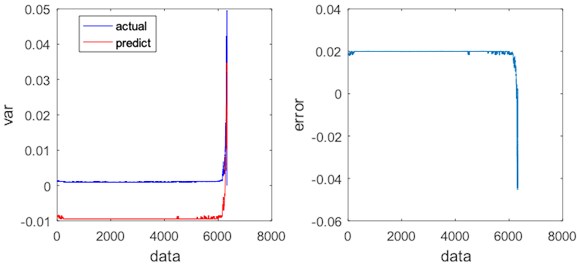
Fig. 18Regression results and errors of LSTM
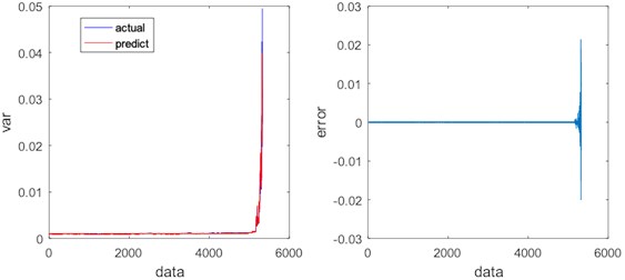
Fig. 19Regression results and errors of ANN
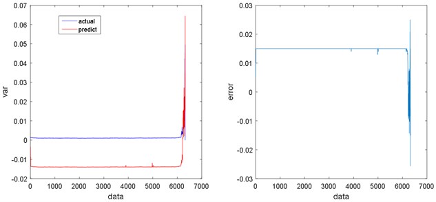
Fig. 20Regression results and errors of KNN
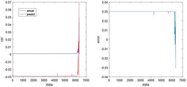
Table 2Absolute total errors of regression methods
Regression algorithm | Absolute total errors |
LSTM regression | 0.4828 |
PSO-SVR regression | 65.6896 |
ANN regression | 92.9650 |
KNN regression | 187.2420 |
Table 3Variance values under different degrees of faults
Degrees of faults | Variance values (10exp(-3)) |
Slight bearing fault | 0.001541 |
Medium bearing fault | 7.066 |
Serious bearing fault | 18.41 |
Fig. 21Analysis chart of rolling bearing data
a)
b)
c)
d)
5. Conclusions
After a depth analysis of the VMD algorithm, it was found that the VMD algorithm had two shortcomings. The center frequency is easy to fall into the local optimum, and the selection of the decomposition layer is poorly adaptive. For these two shortcomings, the VMD center frequency is optimized by the CS algorithm, which can avoid falling into the local optimum. The number of decomposition layers can be reasonably selected by the instantaneous frequency theory. For the timing-related properties of rolling bearing signals, it was proposed to apply the LSTM to the life prediction of rolling bearings, which can effectively improve the regression accuracy of the signal.
Finally, this paper proposes to combine the improved VMD algorithm with the LSTM as a method to study the performance assessment of rolling bearings, and experimenting with the full-life bearing data at the University of Cincinnati, USA. The experimental results show that compared with the traditional methods, the method has obvious advantages in the performance evaluation of rolling bearings.
References
-
Xu Z. H., Ma L. Y. Fault feature extraction of rolling bearings. Ordnance Industry Automation, Vol. 23, Issue 1, 2004, p. 46-48.
-
Wang H. C., Chen J., Dong G. M. Feature extraction of weak faults of rolling bearings based on minimum entropy deconvolution and sparse decomposition. Journal of Mechanical Engineering, Vol. 49, Issue 1, 2013, p. 88-94.
-
Chen L., Tan J. W., Guan H. Evaluation of performance degradation of rolling bearings based on single-layer SAE and SVM. Machine Tool and Hydraulics, Vol. 46, Issue 17, 2018, p. 164-168.
-
Cerrada M., Sánchez R. V., Li C., Pacheco F., Cabrera D. R., Oliveira J. V., Vasquez R. E. Review on data-driven fault severity assessment in rolling bearings. Mechanical Systems and Signal Processing, Vol. 99, 2018, p. 169-196.
-
Huo Z., Zhang Y., Francq P., Shu L., Huang J. F. Incipient fault diagnosis of roller bearing using optimized wavelet transform based multi-speed vibration signatures. IEEE Access, Vol. 5, 2017, p. 19442-19456.
-
Li Y., Liang X., Xu M., Huang W. Early fault feature extraction of rolling bearing based on ICD and tunable Q-factor wavelet transform. Mechanical Systems and Signal Processing, Vol. 86, 2017, p. 204-223.
-
Wu Z. H., Huang N. E. Ensemble empirical mode decomposition: noise-assisted data analysis method. Advances in Adaptive Data Analysis, Vol. 1, Issue 1, 2011, p. 1-41.
-
Smith J. S. Local mean decomposition and its application to EEG perception data. Journal of the Royal Society Interface, Vol. 2, Issue 5, 2005, p. 443-454.
-
Dragomiretskiy K., Zosso D. Variational mode decomposition. IEEE Transactions on Signal Processing, Vol. 62, Issue 3, 2014, p. 531-544.
-
Wang Y., Markert R., Xiang J., Zheng W. Research on variational mode decomposition and its application in detecting rub-impact fault of the rotor system. Mechanical Systems and Signal Processing, Vol. 60, Issue 61, 2015, p. 243-251.
-
Zhang M. L., Zhou Z. H. ML-KNN: lazy learning approach to multi-label learning. Pattern Recognition, Vol. 40, Issue 7, 2007, p. 2038-2048.
-
Li L., Wang H. M., Zhao C. H. Integration method for rolling bearing fault diagnosis. Advanced Materials Research, Vol. 228, Issue 229, 2011, p. 293-298.
-
Elish Mahmoud O. Comparative study of fault density prediction in aspect-oriented systems using MLP, RBF, KNN, RT, DENFIS and SVR models. Artificial Intelligence Review, Vol. 42, Issue 4, 2014, p. 695-703.
-
Patel J. P., Upadhyay S. H. Comparison between artificial neural network and support vector method for a fault diagnostics in rolling element bearings. Procedia Engineering, Vol. 144, 2016, p. 390-397.
-
Yang X. S., Deb S. Cuckoo Search via Lévy flights. World Congress on Nature and Biologically Inspired Computing, 2009, p. 210-214.
-
Viswanathan G. M., Bartumeus F., Buldyrev S. V., Catalan J., Fulco U. L., Havlin S., Luz M. G. E., Lyra M. L., Raposo E. P., Stanley H. E. Lévy flight random searches in biological phenomena. Physica A Statistical Mechanics and Its Applications, Vol. 314, Issue 1, 2002, p. 208-213.
-
Chen D. G., Zhang Y. D., Yao C. Y., Lai B. W., Lv S. J. Fault diagnosis based on variational mode decomposition and multi-scale permutation. Computer Integrated Manufacturing System, Vol. 23, Issue 12, 2017, p. 47-55.
-
Xiao Z., Liang P. J. Chinese sentiment analysis using bidirectional LSTM with word embedding. International Conference on Cloud Computing and Security, Springer, Cham, 2016.
-
Lipton Z. C., Berkowitz J., Elkan C. Critical review of recurrent neural networks for sequence learning. arXiv:1506.00019, 2015.
-
Graves A. Supervised Sequence Labeling with Recurrent Neural Networks. Studies in Computational Intelligence, Springer-Verlag Berlin Heidelberg, Vol. 385, 2008.
Cited by
About this article

