A novel wind turbine gearbox fault diagnosis method based on ASO-VMD and NRF

Shan, Mengchen; Liu, Wenyi

doi:10.21595/jve.2020.21316

Journal of Vibroengineering

Browse Journal

Submit article

Published: 30 September 2020

Check for updates

A novel wind turbine gearbox fault diagnosis method based on ASO-VMD and NRF

Mengchen Shan¹

Wenyi Liu²

^{1, 2}School of Mechatronic Engineering, Jiangsu Normal University, Xuzhou, China

²Department of Mechanical and Aerospace Engineering, Case Western Reserve University, Cleveland, Ohio, 44106, USA

Corresponding Author:

Wenyi Liu

Cite the article Download PDF

Downloads 1130

WoS Core Citations 1

CrossRef Citations 1

Abstract

The combination of feature extraction and pattern recognition can make it possible to realize wind turbine gearboxes based on vibration signals. However, these methods need to be constantly adjusted parameters and spend time training when processing different vibration signals, which is time-consuming. Aiming at reducing the number of parameters that need to be adjusted and training time, this paper proposes a variational mode decomposition (VMD) based on atomic search optimization (ASO) and neural random forest (NRF) fault diagnosis model. The parameters of the VMD are adaptively adjusted by the ASO, which has the advantages of less adjustment parameters. After ASO-VMD decomposition, signals will be used as the input of NRF. We evaluate our method on simulation gearbox model which is established by Solidworks and Adams. Experimental results show that our method has faster training speed and higher recognition accuracy without set many parameters manually.

A novel wind turbine gearbox fault diagnosis method based on ASO-VMD and NRF

Highlights

A wind turbine gearbox fault diagnosis method based on ASO-VMD and NRF
The intrinsic mode function (IMF) can retain the effective information to the greatest extent
The IMF is composed of a feature matrix and used for training and recognition of the NRF
The fault diagnosis model is used to identify the motion state of the gearbox
The fault diagnosis model has faster training speed and higher recognition accuracy

1. Introduction

In recent years, resource shortages and environmental degradation have prompted countries to focus on the development of clean energy [1]. With the development of technology, wind power generation has developed rapidly, and the installed capacity of global wind turbines has increased year by year [2]. The speed-increasing gearbox is the important rotating component in the wind turbine drive system. If damage to gears is not found in time when it occurs, it will cause huge damage to the wind turbine equipment [3, 4].

Time-frequency analysis has been applied to fault diagnosis successfully. Through feature extraction of gearbox vibration signal, the fault information of the gearbox will be extracted. In the field of gearbox vibration signal diagnosis, there are several commonly methods including continuous wavelet transform (CWT) [5, 6], Hilbert-Huang transform (HHT) [7, 8], empirical mode decomposition (EMD) [9] and local mode decomposition (LMD) [10]. However, CWT depend on the selection of wavelet basis function. When analyze different signal, we need to select different wavelet basis function. In the decomposition process of EMD and LMD, mode mixing and endpoint effect affect the result [11]. Variational mode decomposition (VMD) [12] is a fault adaptive processing method proposed by Dragomireskiy et al. Due to its good anti-noise ability, VMD has been widely used in the field of fault diagnosis [13-16]. Although VMD has good signal decomposition capability, VMD needs to set more parameters during use. If the parameter settings are unreasonable, the signal decomposition result will be poor. A common solution is to use the parameter optimization method to select the optimal parameters of the VMD. Lv et al. [17] decomposes the fault signal through VMD, it uses the support vector machine (SVM) based on genetic algorithm to identify the fault and improve the generalization ability of the model; Yi et al. [18] use particle swarm optimization (PSO) to find the optimal parameters of VMD to realize Bearing fault diagnosis; Wang et al. [19] use PSO to minimize the average envelope entropy method to optimize the parameters of VMD; J Zhu [20] uses the artificial fish algorithm (AFSA) to find the optimal parameters of VMD to realize the fault diagnosis of rolling bearings; Wang [21] et al. used symbol dynamic entropy and power spectral entropy as fitness functions, and used multi-objective particle swarm optimization (MOPSO) to find the optimal parameters of VMD; Miao et al. [22] used the kurtosis of the indicator set as the objective function. Use the locust optimization algorithm (GOA) to optimize the objective function and select the best VMD parameters. Although the parameter optimization method is used to select the optimal parameters of the VMD, the optimization method itself still needs to set more parameters, and the parameters have a greater impact on the results, which leads to a large number of experiments to determine the optimal parameter range, increasing the difficulty of the experiment. The Atomic Search Optimization Algorithm (ASO) [23] requires fewer parameters to be set and guarantees optimization. At present, ASO is rarely used in the field of mechanical fault diagnosis.

After the signal is decomposed by the VMD, it still contains a variety of vibration information during the operation of the device. Therefore, a suitable pattern recognition method is needed to further determine the type of the fault. Common pattern recognition methods such as support vector machine [24, 25], artificial neural network [26-28] etc., are widely used in mechanical equipment fault diagnosis, and have achieved remarkable results. Li et al. [29] use a deep belief networks (DBN) to classify the gearbox failure; Chen et al. [30] extracted signals features and use CNN to determine the state of the gearbox. Verma et al. [31] use the extraction of time and frequency features as input for a spare auto-encoder (SAE). Shao et al. [32] use optimize DBN and time-domain features to diagnose faults of bearings. Janssens et al. [33] explored that CNN used the original frequency data to diagnose the bearing seat. The vibration data of the bearing box is pre-processed by Fast Fourier Transform (FFT) and input into CNN to detect faults. However, the above pattern recognition methods all have slow training speeds and are prone to over-fitting problems. Neural random forest (NRF) [34] is a pattern recognition method proposed by Biau et al. in 2016, and NRF is a hybrid method that converts random forest (RF) into a neural network (NN). Compared with RF and NN, NRF requires fewer parameters than standard networks, and there are fewer restrictions on decision geometry than RF.

Aiming at the difficulty of VMD parameter optimization and time-consuming training in fault diagnosis model, this paper proposes a fault diagnosis model based on ASO-VMD and NRF. The ASO is used to select the optimal decomposition parameter of the VMD, under which the original fault signal is decomposed using VMD. The principal component analysis (PCA) is used to perform dimensional compression on the decomposed signal, and finally NRF is used for classification and identification to realize fault diagnosis of the gearbox. Compared with the above method, our proposed method only needs to set two parameters in the process of optimizing VMD. At the same time, in the final fault identification effect, the recognition accuracy of the method reaches 100 %, which can meet the actual fault diagnosis requirements.

2. Fault diagnosis model

2.1. Model workflow

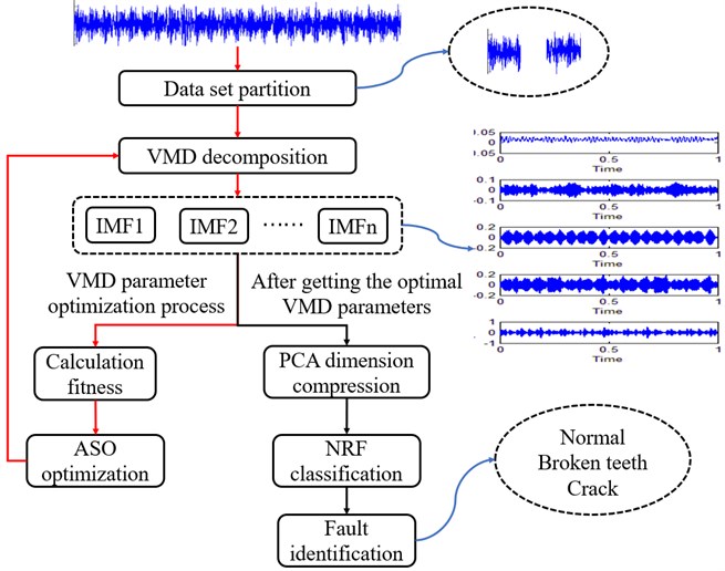
Aiming at the gear failure in wind turbine gearbox, this paper proposes an intelligent fault diagnosis model based on ASO-VMD and NRF. The training and working process of the model is shown in Fig. 1.

In this paper, the fault signal of the wind turbine is obtained by Solidworks and Adams simulation [35]. The model built in the simulation is the gearbox of a 1.5 MW wind turbine. Its structure is a set of planetary wheels and two sets of parallel wheels. The collected original simulation signals are divided into several signals. Each segment of the signal is decomposed by ASO-VMD and the total signal fitness is obtained. In this process ASO will optimize the parameters of VMD according to fitness function, which will be described in Section 2.3. The signal decomposed by ASO-VMD has higher dimensions. Before using NRF to classify the signal, we use PCA to reduce the dimensions. Finally, the NRF can accurately identify the gearbox fault status and use other test data to verify the model effect after training.

Fig. 1Model workflow

2.2. Basic principles of VMD

VMD is a new type of adaptive decomposition method for nonlinear non-stationary signals developed in recent years. VMD can decompose the signal $f (t)$ into multiple eigenmode functions (IMF), and the IMF is defined as shown in Eq. (1):

1

u_{k} (t) = A_{k} (t) \cos (φ_{k} (t)) .

In the VMD decomposition, the signal $f (t)$ updates the IMF center frequency and bandwidth by iteration. Assuming that each eigenmode function $u_{k} (t)$ is the finite bandwidth of the center frequency, this variational problem can be transformed into a constrained variational problem that seeks $k$ eigenmode function IMFs. The constrained variational model is described as Eqs. (2-3):

2

\underset{{u_{k}}, {ω_{k}}}{m i n} \{{\sum_{k} ‖\partial_{t} [(σ (t) + \frac{j}{π t}) u_{k} (t)] e^{- j ω_{k} t}‖}_{2}^{2}\},

3

s . t . \sum_{k} u_{k} = f .

In order to find the optimal solution of the above constrained variational problem, the augmented Lagrange function can be constructed by introducing the quadratic penalty factor $α$ and the Lagrange multiplication operator $λ (t)$ . The Lagrange function is time-frequency transformed, and corresponding solutions are obtained to obtain expressions of the modal function components $u_{k}$ and $ω_{k}$ , respectively. Then use the alternating direction multiplier algorithm to find the optimal solution of the constrained variational model, and then decompose the original signal into multiple IMFs.

2.3. ASO-based VMD

Inspired by molecular dynamics, ASO achieves the optimal solution of the parameter optimization problem by mathematically simulating the motion of atoms in nature. The ASO initially randomly generates the position of each atom, and the atom updates their position and velocity in each iteration until the best position of the atom is found, which is the optimal solution of the objective function. The acceleration of an atom is determined by two factors: the mutual interaction between atoms and the binding force caused by the bond length potential. The optimal atomic position is taken as the optimal solution for parameter optimization after the end of the iteration. In the ASO algorithm, the position and velocity of each atom are randomly generated first, and the atomic fitness is initialized. Determine the $K$ neighborhood of each atom, and determine the $K$ neighborhood as defined by Eq. (4):

4

K (t) = N - (N - 2) \times \sqrt{\frac{t}{T}},

where $t$ is the number of iterations, $N$ is the number of atoms, and $T$ is the total number of iterations. Through the $K$ neighborhood, the amount of calculation can be effectively reduced, and the iteration speed can be improved. In each of the original neighborhoods, calculate the force and binding force between them and other atoms, wherein the force calculation formula is as shown in Eqs. (5-6):

5

F_{i}^{d} (t) = \sum_{j \in K b e s t} {r a n d}_{j} F_{i j}^{d} (t),

6

F_{i j} = - \nabla U (r_{i j}) = \frac{24 ε}{σ^{2}} [2 {(\frac{σ}{r_{i j}})}^{14} - {(\frac{σ}{r_{i j}})}^{8}] r_{i j},

where $r_{i j}$ represents the spatial position between two atoms, $ε$ represents the strength of the interaction, and $σ$ represents the length scale of the collision diameter. The formula for calculating the binding force is as shown in Eqs. (7-8):

7

G_{i}^{d} (t) = - λ (t) \nabla θ_{i}^{d} (t) = - 2 λ (t) (x_{i}^{d} (t) - x_{b e s t}^{d} (t)),

8

θ_{i} (t) = [{|x_{i} (t) - x_{b e s t} (t)|}^{2} - b_{i, b e s t}^{2}],

where $λ (t)$ is the Lagrangian multiplication, $x_{i} (t)$ is the optimal atomic position in each iteration, and $b$ is the fixed length between the $i$ th atom and the best atom.

The force of each atom is iterated to calculate the acceleration of each atom, and the position of each atom is updated by the acceleration. After each iteration is completed, the fitness value $F_{i t}$ is calculated. After the end of the iteration, the minimum fitness value is selected as the optimal solution, and the atomic position and variables at the optimal time are calculated.

When using VMD decomposition, parameters need to be set according to prior experience, but the signal in the gearbox is complex, and setting parameters according to experience cannot ensure that the VMD can accurately identify the fault features. Therefore, an atomic optimization algorithm is used to select the optimal parameters. The parameters to be selected in the VMD are the penalty factor $α$ and the number $K$ of narrowband modal components. Each group of signals is decomposed by VMD to obtain $K$ IMFs, and the information difference coefficient $A$ between the IMFs is calculated, as in Eqs. (9-10) shown:

9

A = {(S_{1} - S)}^{2} + {(S_{2} - S)}^{2} + \dots + {(S_{K} - S)}^{2},

10

S = \sum_{i}^{K} \frac{S_{i}}{K},

where $S_{i}$ represents the information entropy of each IMF. The error coefficient e of the initial signal and the reconstructed signal is defined as shown in Eq. (11):

11

e = s u m [a b s (f - x_{1} - x_{2} - \dots x_{K})],

where $f$ denotes the initial signal, and $x_{K}$ indicates the decomposed signal. The VMD decomposition fitness is expressed as shown in Eq. (12):

12

ρ = \frac{e}{A} .

The larger the $A$ value, the greater the amount of information contained in each IMF. The larger the $A$ value, the more information the IMF contains. The smaller the $e$ value, the more similar the reconstructed signal is to the original signal. Since the fault information contained in each group of signals in the data set is inconsistent, the fitness of the gearbox in each state is added, as shown in Eq. (13):

13

P = \sum_{i}^{I} ρ_{i} .

$P$ is the total fitness of the signal, and $I$ is the total number of signals. Taking this as the objective function of the atomic optimization algorithm, the minimum value of $P$ and the $K$ and $α$ at this time are obtained through multiple iterations.

2.4. PCA

Gearbox fault signals still have a high dimension after VMD decomposition, which is not conducive to subsequent signal characteristic analysis. Therefore, PCA is used to compress high-dimensional data and retain feature points that have a large impact on the results. The principle of PCA is to transform the original data in high-dimensional space to obtain the transformation direction with the largest variance, so as to achieve dimensional compression. Before using PCA, the time domain signals in each state are composed into a matrix $X$ :

14

X = [\begin{matrix} x_{11} & \dots & x_{1 m} \\ ⋮ & ⋱ & ⋮ \\ x_{n 1} & \dots & x_{n m} \end{matrix}],

where $n$ is the number of samples and $m$ is the number of features. Normalize each feature point in the sample and calculate the correlation coefficient matrix, as Eqs. (15-16) shown:

15

x_{i, j} = \frac{x_{i j} - \min x_{j}}{\max x_{j} - \min x_{j}},

16

R = [\begin{matrix} r_{11} & \dots & r_{1 m} \\ ⋮ & ⋱ & ⋮ \\ r_{n 1} & \dots & r_{n m} \end{matrix}] .

Finally calculate the special diagnosis vector of the correlation coefficient matrix, as in Eq. (17) shown:

17

|λ I - R| = 0 .

After the feature vector is obtained, the first 1024 features of the cumulative variance contribution rate are selected as the main indicators for subsequent analysis.

2.5. Basic principles of NRF

Based on the decision tree algorithm, the random forest combines multiple decision trees at the same time, and combines the results of multiple decision trees with the least empirical error method to obtain the optimal results. The literature [34] pointed out that the decision tree can be seen as a two-layer neural network model. For each layer of the neural network, its activation function is shown in Eq. (18):

18

τ (h_{k} (x)) = τ (x^{(j_{k})} - α_{j_{k}}),

where $τ (u) = 21 u \geq 001$ is the threshold activation function. The weight and paranoia of each layer are related to the decision tree model. The final output of the neural network is shown in Eq. (19):

19

t_{n} (x) = \sum_{k^{'} = 1}^{K} w_{k^{'}} v_{k^{'}} (x) + b_{o u t} .

The conversion relationship between decision tree and neural network is shown in Fig. 2.

In a random forest, the results of all decision trees will be aggregated to form a forest assessment, as shown in Eq. (20):

20

t (x; θ_{1}, \dots, θ_{m}, D_{n}) = \frac{1}{M} \sum_{m = 1}^{M} t (x; θ_{m}, D_{n}) .

After replacing the decision tree with a neural network, all the results are summarized by a random forest method, and finally a neural random forest model is formed.

Fig. 2Stochastic neural network [34]

3. Wind turbine gearbox modeling

In order to verify the effectiveness of the ASO-VMD and NRF fault diagnosis models. We establish the wind turbine gearbox simulation model and collect the vibration signal of the gearbox during operation.

3.1. Gearbox modeling

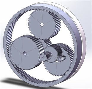
Large wind turbine gearboxes are generally composed of planetary gear trains and parallel gear trains. In 1.5 MW wind turbine gearboxes, the common structure is composed of a set planet gears and two sets parallel gears, which can reduce the risk of gearbox failure. According to references [36], the input speed of the wind turbine gearbox is generally 10-30 r/min, and the output speed is generally 1500 r/min. Based on the above situation, the total gear ratio of our simulated gearbox is 100.8, and the parallel gears consist of helical gears. The gear parameters of each stage are shown in Table 1.

Table 1Gearbox parameters

	Planetary train			Parallel gear train 1		Parallel gear train 2
	Sun gear	Planetary wheel	Ring gear	Large gear	Small gear	Large gear	Small gear
Modulus	22	22	22	14	14	10	10
Number of teeth	26	55	136	92	21	63	17
Index circle diameter	572 mm	1210 mm	2992 mm	1288 mm	294 mm	630 mm	170 mm

The gearbox model is established by Solidworks. In order to simplify the calculation of the simulation, the part between the transmission shaft and the gear transmission is omitted in the model. The modeling result of the gearbox is shown in Fig. 3.

Fig. 33D model of the gearbox

3.2. Fault simulation

The fault types of the gears in the wind turbine gearbox generally include broken teeth, pitting, and cracks. Among them, gear cracks and broken teeth cause more damage to the gearbox. If it cannot be found in time, it will have a huge impact on the normal operation of the wind turbine. In order to find the vibration characteristics of the gearbox when gear cracks or broken teeth, dynamic simulation of the gearbox is required. The gearbox 3D model is imported into Adams, and the basic constraints and flexibility settings are made for each gear.

A contact force is set between the respective gears, and the input speed of the gearbox is set to 0.66 π/s, a resistance of 6000 N⋅m is set at the output end. In the Adams simulation setup, the simulation time is set to 5 s, the number of simulation steps is 20,000 steps, and the damping factor of the flexible body is set to 50. The meshing frequency of each gear can be calculated by combining the above simulation conditions. The results are shown in Table 2.

Table 2Gear meshing frequency of each stage

	Planetary train			Parallel gear train 1		Parallel gear train 2
	Sun gear	Planetary wheel	Ring gear	Large gear	Small gear	Large gear	Small gear
Rotating speed °/s	740	175	0	740	3241	3241	12010
Meshing frequency / Hz	53	26.73	0	189		567

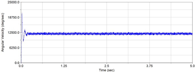
Firstly, we verify the gears ratio of the gearbox. The output speed is shown in Fig. 4. It can be seen from the figure that the system enters a steady state after about 0.2 s. The average angular velocity is 12000 °/s and the range of fluctuation of the speed is less than 100 °/s, which satisfies the characteristics of the periodic meshing impact of the gear and conforms to the display.

Fig. 4Output speed

In order to reduce the interference of other vibration source, the vibration sensor is generally placed at the input and output ends of the gearbox in the actual working environment [37, 38]. Therefore, the vibration signal of the output gear is collected in the Adams simulation environment, and the acceleration time domain signal and the frequency domain signal are shown in Fig. 5.

Fig. 5Output frequency vibration signal frequency domain diagram

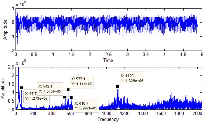
It can be seen from the frequency domain diagram that frequency corresponding to amplitude is very close to the theoretical gear frequency, thus verifying the validity of the model.

In order to verify that the model can simulate the vibration characteristics of the gearbox failure, the normal gears in the model are replaced with gears of different fault types. In the test, the large gears in the sun gear and the parallel gears train 2 are replaced by broken gears. The models of the fault gears are shown in Fig. 6. The crack is set to have a split width of 2.5 mm and a depth of 3 mm.

Fig. 6Gear failure model

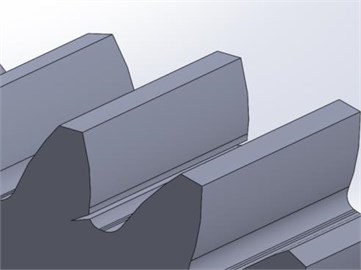
a) Tooth root crack

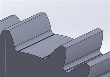
b) Broken tooth

In the Adams model, the normal gear is replaced by the faulty gear, the model simulation time is set to 5 s, and the number of simulation steps is 20,000 steps. The time-frequency domain signals of the output terminals under different faults are shown in Fig. 7.

Fig. 7Frequency domain diagram of parallel gear train 2 large gear broken teeth

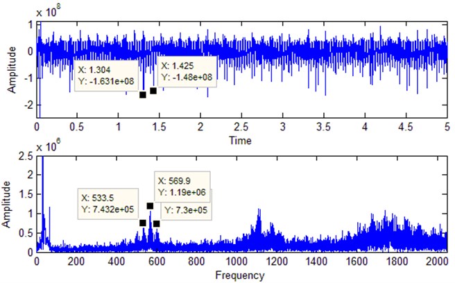
Fig. 7 shows the time-frequency domain diagram of the 2 large gears of the parallel gear train in the state of broken teeth. Compared with the normal state, the time domain diagram under the broken tooth state has obvious periodic impact. The time interval between two adjacent impacts is 0.121, and the corresponding frequency is 8.3 Hz. This is close as the parallel gear train 2 which the gear rotation frequency is 9 Hz. In the frequency domain signal, the meshing frequency of the parallel gear train 2 basically matches the signal amplitude in the frequency domain diagram. At the same time, compared with the frequency domain diagram under normal conditions, the amplitude at the meshing frequency has increased significantly. This can further verify the accuracy of the simulation model. On this basis, the vibration signals of the gear box body and the output end in other fault states are collected separately as the input of the fault diagnosis model. The data amount in the state of each gear box will be described in detail in Section 4.1.

4. Experiment analysis

4.1. Fault diagnosis model establishment

The workflow of the wind turbine gearbox fault diagnosis model has been described in detail in the previous section. The detailed parameters of each part in the model are described below.

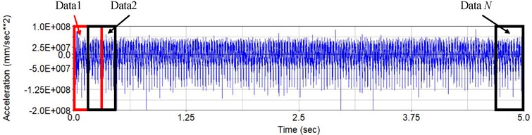
(1) The simulation time of the gearbox is 5 s, and the number of sampling points is 20,000. There are two sets of vibration data in the same state: ring gear vibration data and output vibration data. The data will be divided into several groups by sliding method, the length of each group is 4096. Each set of data has a size of 2×4096. The data set includes the normal state of the gearbox, the single gear broken teeth, and the crack fault state. Multiple gears have multiple fault conditions at the same time. The total number of samples divided into total is 575 groups. The data set is divided as shown in Fig. 8.

Fig. 8Data set partitioning (sliding method example)

(2) The number of atoms in the ASO is set to 10, the maximum number of iterations is set to 50, the search range of $K$ is [2, 10], and the search range of $α$ [100, 6000] s.

(3) Select the optimal parameters obtained by the optimization algorithm, and decompose the samples with VMD. After each group of data is decomposed, a feature matrix of $(m, 2 K \times 4096)$ is obtained, where m is the number of samples. The feature matrix is dimensionally compressed by PCA, and the effective features are extracted. The dimension of the feature matrix after compression by principal component analysis is $(m, 1024)$ .

(4) Put the special diagnosis matrix into the nerve random forest for training. 50 % of the data in each state of the data set is used as the training set, 25 % is used as the verification set, and 25 % is used as the test set. The number of data sets in each state is shown in Table 3.

Table 3Number of data sets

	Number of training sets	Number of verification sets	Number of test sets	Total amount
Gearbox is normal	31	16	16	63
Sun wheel crack	37	18	18	73
Parallel wheel crack	41	21	21	83
Sun gear broken teeth	113	57	57	227
Parallel wheel breaking	32	16	16	64
Multi-gear broken teeth	33	16	16	65

In the NRF, a total of 30 class decision trees are set. The neural network has two hidden layers, of which the first layer contains 20 nodes and the second layer contains 10 nodes. The maximum number of iterations of the model is 100.

4.2. ASO-VMD decomposition result

In order to check the effectiveness of the ASO-VMD algorithm, the method is compared with the PSO-VMD [18] and AFSA-VMD [20] method. PSO needs to set parameters such as the number of particles, the inertia factor, and the maximum flying speed. AFSA needs to set parameters such as the number of artificial fish, the maximum number of trials, the perceived distance, and the congestion factor. Compared to PSO and AFSA, ASO only needs to set the initial number of atoms and the number of iterations to achieve VMD optimization, which minimizes the impact of setting parameters on the results. As shown in Table 4, different VMD optimization parameters are obtained by different optimization algorithms. The PSO and AFSA parameters are set to be basically the same as the ASO to improve the experimental contrast.

Table 4VMD parameters and their correlation under different optimization algorithms

	$K$	$α$	Correlation coefficient	Total fitness
PSO optimization	8	100	0.983	17.41
AFSA optimization	10	700	0.9795	25.64
ASO optimization	10	200	0.990	14.31

It can be seen from the table that compared with the PSO-VMD and AFSA-VMD, the ASO-VMD processed signal has a better correlation with the original signal, and the fault features are decomposed while maximally retaining the signal. Information, while ASO-VMD has a better fitness value than PSO-VMD and AFSA-VMD.

Fig. 9Optimization algorithm iterative process

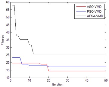
As shown in Fig. 9, the iterative process of ASO-VMD shows that ASO-VMD has found the optimal parameters in about 20 rounds. In PSO-VMD, the fitness value in the iterative process is at least about 17, the minimum value of AFSA-VMD is only 25.64. It can be seen that ASO-VMD has better ability to prevent local minimization, and its optimization result is better.

Fig. 10 shows the positional changes of 10 atoms in the 50-pass iteration of ASO. It can be seen from the figure that the atomic distribution is scattered at the initial iteration, ensuring that a large range of space can be searched. As the iterative process progresses, the atoms gradually enter an equilibrium state, the distribution of atoms begins to concentrate, eventually reaching a stable range.

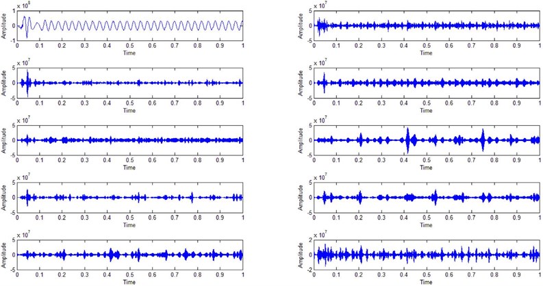
The time domain map of each IMF after decomposition by ASO-VMD is shown in Fig. 11. It can be seen from the figure that the characteristics of each IMF time domain signal are obvious. Since each IMF represents a part of the vibration information in the original signal, the original signal contains the vibration information of the original signal after being decomposed by the ASO-VMD. It is decomposed into each IMF, making the individual vibration components of the original signal easier to identify, which is beneficial to the use of subsequent fault identification methods.

Fig. 10ASO-VMD atomic changes

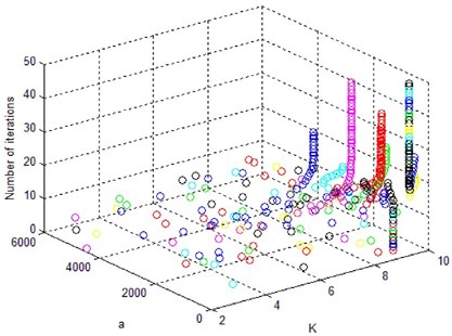
Fig. 11IMF time domain map

4.3. Fault identification verification

From the decomposition effect point of view, the effect of ASO-VMD and PSO-VMD is closer, so we put the signals decomposed by ASO-VMD and PSO-VMD into NRF for training. At the same time, the same neural network model and NRF are compared. The comparison indicators include model accuracy and root mean square error. The training results are shown in Table 5.

Table 5Cumulative recognition accuracy of different model tests

	ASO-VMD		PSO-VMD
	Accuracy	Root mean square error	Accuracy	Root mean square error
Random forest	100 %	1.21	100 %	1.32
BP Neural Networks	88 %	19.48	86 %	21.32
NRF	100 %	1.17	100 %	1.21

From the table we can see that the signal decomposed by ASO-VMD has higher accuracy and smaller root mean square error under each recognition model. At the same time, under the same parameter configuration, both NRF and RF have a higher recognition rate after rounding the value of the network output. However, from the perspective of root mean square error, the NRF output is closer to the actual value, and the model has a more stable and accurate output.

The accuracy rate changes between different models in the training process are compared, and the variation curves are shown in Fig. 12.

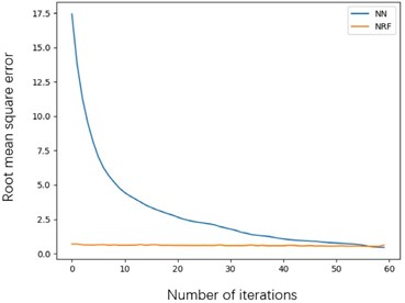
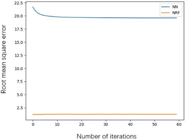
Fig. 12Root mean square error curve of a) validation set and b) test set

a)

b)

It can be seen from the figure that during the training process, the initial error of the neural network is large. After 60 iterations, the error is smaller than the random forest of the nerve, and the training set achieves better results. However, in the verification set, although the neural network realized the gradient decline in the previous rounds of iteration, the root mean square is always stable at around 20, so it can be seen that the neural network has experienced a serious over-fitting situation. However, the neural randomization still maintains a low error in the verification set. It can be seen that the NRF forest has faster training speed and better test results than the neural network.

Table 6Identification accuracy of different models

Decomposition algorithm	Classification algorithm	Accuracy
ASO-VMD	NRF	100 %
VMD (center frequency method to select parameters)	NRF	93.75 %
EMD	NRF	90.3 %
ASO-VMD	CNN	97.2 %
VMD	CNN	91.0 %
EMD	CNN	90.3 %
ASO-VMD	SVM	22.9 %
VMD	SVM	22.9 %
EMD	SVM	27.1 %
/	BP neural networks	84.0 %
/	CNN	95.8 %

Our method is mainly composed of decomposition algorithm and classification algorithm, both of which directly have different methods to replace. The accuracy of data classification by the combination if different methods is shown in Table 6. We have manually tuned all models to achieve the best results. Among the existing fault diagnosis models, there are pattern recognition technologies such as CNN to achieve end-to-end fault diagnosis [27]. We also compared the end-to-end fault diagnosis model. From Table 6 we can see that ASO-VMD-NRF can achieve the best results. The VMD based on the center frequency method adjusts parameters cannot achieve the best decomposition effect for all signals, resulting in a decrease in accuracy. In the ASO-VMD-CNN model, some of the decomposed signal features are similar. Due to the poor generalization ability of CNN compared to NRF, a wrong judgment is generated.

5. Conclusions

This paper presents a gearbox fault diagnosis model and tests the effect of the model in a simulation environment. The model has the following characteristics:

1) ASO can realize the VSD adaptive decomposition signal, reduce the subjective error caused by human adjustment, and the ASO needs less adjustment parameters, which reduces the difficulty caused by adjusting parameters. The experimental results show that the ASO-VMD can effectively remove the noise in the signal and preserve the effective information components in the signal to the greatest extent.

2) NRF has faster training speed and lower recognition error than neural network or random forest. Under the same parameter structure, NRF can achieve more stable recognition accuracy while avoiding over-fitting.

3) ASO-VMD and NRF as an adaptive fault diagnosis model can accurately determine the type of gearbox failure. This paper verifies the effectiveness of the model through the gearbox simulation model. It provides a stable and accurate solution for wind turbine gear fault diagnosis.

In the next work, we will further expand the model’s fault identification capability under non-steady state and study the model’s fault identification capability under dynamic load environment.

References

Fogaing M., Gordon H., Lange C., et al. A Review of Wind Energy Resource Assessment in the Urban Environment, Advances in Sustainable Energy. Springer, Cham, 2019, p. 7-36.

Publisher
Kumar Y., Ringenberg J., Depuru S., et al. Wind energy: trends and enabling technologies. Renewable and Sustainable Energy Reviews, Vol. 53, 2016, p. 209-224.

Publisher
Márquez F., Tobias A., Pérez J., et al. Condition monitoring of wind turbines: techniques and methods. Renewable Energy, Vol. 46, 2012, p. 169-178.

Publisher
Liu W.Y., Tang B.P., Han J.G., et al. The structure healthy condition monitoring and fault diagnosis methods in wind turbines: a review. Renewable and Sustainable Energy Reviews, Vol. 44, 2015, p. 466-472.

Publisher
Zheng H., Li Z., Chen X. Gear fault diagnosis based on continuous wavelet transform. Mechanical Systems and Signal Processing, Vol. 16, Issues 2-3, 2002, p. 447-457.

Publisher
Rafiee J., Rafiee M. A., Tse P. W. Application of mother wavelet functions for automatic gear and bearing fault diagnosis. Expert Systems with Applications, Vol. 37, Issue 6, 2010, p. 4568-4579.

Publisher
Cheng G., Cheng Y., Shen L., et al. Gear fault identification based on Hilbert–Huang transform and SOM neural network. Measurement, Vol. 46, Issue 3, 2013, p. 1137-1146.

Publisher
Yu X., Ding E., Chen C., et al. A novel characteristic frequency bands extraction method for automatic bearing fault diagnosis based on Hilbert Huang transform. Sensors, Vol. 15, Issue 11, 2015, p. 27869-27893.

Publisher
Li Y., Xu M., Wei Y., et al. An improvement EMD method based on the optimized rational Hermite interpolation approach and its application to gear fault diagnosis. Measurement, Vol. 63, 2015, p. 330-345.

Publisher
Cheng J., Zhang K., Yang Y. An order tracking technique for the gear fault diagnosis using local mean decomposition method. Mechanism and Machine Theory, Vol. 55, 2012, p. 67-76.

Publisher
Zhang L., Wang Z., Quan L. Research on weak fault extraction method for alleviating the mode mixing of LMD. Entropy, Vol. 20, Issue 5, 2018, p. 387.

Publisher
Dragomiretskiy K., Zosso D. Variational mode decomposition. IEEE Transactions on Signal Processing, Vol. 62, Issue 3, 2013, p. 531-544.

Publisher
Wang Y., Markert R., Xiang J., et al. Research on variational mode decomposition and its application in detecting rub-impact fault of the rotor system. Mechanical Systems and Signal Processing, Vol. 60, 2015, p. 243-251.

Publisher
Zhao H., Li L. Fault diagnosis of wind turbine bearing based on variational mode decomposition and Teager energy operator. IET Renewable Power Generation, Vol. 11, Issue 4, 2017, p. 453-460.

Publisher
Li Z., Jiang Y., Guo Q., et al. Multi-dimensional variational mode decomposition for bearing-crack detection in wind turbines with large driving-speed variations. Renewable Energy, Vol. 116, 2018, p. 55-73.

Publisher
Liu W. Y. A review on wind turbine noise mechanism and de-noising techniques. Renewable Energy, Vol. 108, Issue 8, 2017, p. 311-320.

Publisher
Lv Z., Tang B., Zhou Y., et al. A novel method for mechanical fault diagnosis based on variational mode decomposition and multikernel support vector machine. Shock and Vibration, Vol. 2016, 2016, p. 3196465.

Publisher
Yi C., Lv Y., Dang Z. A fault diagnosis scheme for rolling bearing based on particle swarm optimization in variational mode decomposition. Shock and Vibration, Vol. 2016, 2016, p. 9372691.

Publisher
Wang X. B., Yang Z. X., Yan X. A. Novel particle swarm optimization-based variational mode decomposition method for the fault diagnosis of complex rotating machinery. IEEE/ASME Transactions on Mechatronics, Vol. 23, Issue 1, 2017, p. 68-79.

Publisher
Zhu J., Wang C., Hu Z., et al. Adaptive variational mode decomposition based on artificial fish swarm algorithm for fault diagnosis of rolling bearings. Proceedings of the Institution of Mechanical Engineers, Part C: Journal of Mechanical Engineering Science, Vol. 231, Issue 4, 2017, p. 635-654.

Search CrossRef
Wang Z., He G., Du W., et al. Application of parameter optimized variational mode decomposition method in fault diagnosis of gearbox. IEEE Access, Vol. 7, 2019, p. 44871-44882.

Search CrossRef
Miao Y., Zhao M., Lin J. Identification of mechanical compound-fault based on the improved parameter-adaptive variational mode decomposition. ISA Transactions, Vol. 84, 2019, p. 82-95.

Publisher
Zhao W., Wang L., Zhang Z. Atom search optimization and its application to solve a hydrogeologic parameter estimation problem. Knowledge-Based Systems, Vol. 163, 2019, p. 283-304.

Publisher
Widodo A., Yang B. S. Support vector machine in machine condition monitoring and fault diagnosis. Mechanical Systems and Signal Processing, Vol. 21, Issue 6, 2007, p. 2560-2574.

Publisher
Liu W., Wang Z., Han J., et al. Wind turbine fault diagnosis method based on diagonal spectrum and clustering binary tree SVM. Renewable Energy, Vol. 50, 2013, p. 1-6.

Publisher
Jia F., Lei Y., Guo L., et al. A neural network constructed by deep learning technique and its application to intelligent fault diagnosis of machines. Neurocomputing, Vol. 272, 2018, p. 619-628.

Publisher
Zhang W., Li C., Peng G., et al. A deep convolutional neural network with new training methods for bearing fault diagnosis under noisy environment and different working load. Mechanical Systems and Signal Processing, Vol. 100, 2018, p. 439-453.

Publisher
Chine W., Mellit A., Lughi V., et al. A novel fault diagnosis technique for photovoltaic systems based on artificial neural networks. Renewable Energy, Vol. 90, 2016, p. 501-512.

Publisher
Li C., Sánchez R. V., Zurita G., et al. Fault diagnosis for rotating machinery using vibration measurement deep statistical feature learning. Sensor, Vol. 16, Issue 6, 2016, p. 895.

Publisher
Chen Z. Q., Li C., Sanchez R. V. Gearbox fault identification and classification with convolutional neural networks. Shock and Vibration, Vol. 2015, 2015, p. 390134.

Publisher
Verma N. K., Gupta V. K., Sharma M., et al. Intelligent condition based monitoring of rotating machines using sparse auto-encoders. IEEE Conference on Prognostics and Health Management (PHM), 2013.

Publisher
Shao H., Jiang H., Zhang X., et al. Rolling bearing fault diagnosis using an optimization deep belief network. Measurement Science and Technology, Vol. 26, Issue 11, 2015, p. 115002.

Publisher
Janssens O., Slavkovikj V., Vervisch B., et al. Convolutional neural network based fault detection for rotating machinery. Journal of Sound and Vibration, Vol. 377, 2016, p. 331-345.

Publisher
Biau G., Scornet E., Welbl J. Neural random forests. Sankhya A, Vol. 81, 2019, p. 347-386.

Publisher
Liu W. Y. Design and kinetic analysis of wind turbine blade-hub-tower coupled system. Renewable Energy, Vol. 94, 2016, p. 547-557.

Publisher
Nejad A. R., Odgaard P. F., Moan T. Conceptual study of a gearbox fault detection method applied on a 5-MW spar-type floating wind turbine. Wind Energy, Vol. 21, Issue 11, 2018, p. 1064-1075.

Publisher
Medina R., Macancela J. C., Lucero P., et al. Vibration signal analysis using symbolic dynamics for gearbox fault diagnosis. The International Journal of Advanced Manufacturing Technology, Vol. 104, 2019, p. 2195-2214.

Publisher
Liu W. Y., Han J. G., Lu X. N. Experiment and Performance analysis of the Northwind 100 wind turbine in CASE. Energy and Buildings, Vol. 68, 2014, p. 471-475.

Publisher

Cited by

Method for Denoising the Vibration Signal of Rotating Machinery through VMD and MODWPT

(2023)

About this article

Received

28 January 2020

Accepted

08 May 2020

Published

30 September 2020

SUBJECTS

Fault diagnosis based on vibration signal analysis

DOI

https://doi.org/10.21595/jve.2020.21316

Keywords

wind turbine

fault diagnosis

atomic search optimization

variational mode decomposition

neural random forest

Acknowledgements

This research was supported by the National Natural Science Foundation of China (Grant No. 51505202), the 333 Project of Jiangsu Province (2016-III-2808), the Qing Lan Project of Jiangsu Province (QL2016013), Jiangsu Postgraduate Research and Practice Innovation Program of China (KYCX20_2334).

This is an open access article distributed under the Creative Commons Attribution License, which permits unrestricted use, distribution, and reproduction in any medium, provided the original work is properly cited.

Previous article in issue Previous Next article in issue Next

Research article

2022 08 23

Repetitive impacts recovering using variational mode extraction with constructed reference enhanced by improved blind deconvolution

Wenliao Du, Xukun Hou, Hongchao Wang

Review article

2021 01 27

A review on wind turbines gearbox fault diagnosis methods

H. Gu, W. Y. Liu, Q. W. Gao, Y. Zhang

Research article

2020 12 31

A novel wind turbine fault diagnosis method based on generator current analysis

X. Wang, W. Y. Liu, Y. Zhang, H. Gu

Research article

2019 11 28

Hyperparameter optimization for enabling multi-level feature classification in a wind turbine gearbox

Vamsi Inturi, Karthick Chetti, Shreyas N, Sabareesh G R

M. Shan and W. Liu, “A novel wind turbine gearbox fault diagnosis method based on ASO-VMD and NRF,” Journal of Vibroengineering, Vol. 22, No. 6, pp. 1357–1372, Sep. 2020, https://doi.org/10.21595/jve.2020.21316

Copy Extrica

Copied to clipboard!

TY  - JOUR
DO  - 10.21595/jve.2020.21316
UR  - https://doi.org/10.21595/jve.2020.21316
TI  - A novel wind turbine gearbox fault diagnosis method based on ASO-VMD and NRF
T2  - Journal of Vibroengineering
AU  - Liu, Wenyi
AU  - Shan, Mengchen
PY  - 2020
DA  - 2020/09/30
PB  - JVE International Ltd.
SP  - 1357-1372
IS  - 6
VL  - 22
SN  - 1392-8716
SN  - 2538-8460
ER  - 

Copy Ris

Copied to clipboard!

@article{Liu_2020,
	doi = {10.21595/jve.2020.21316},
	url = {https://doi.org/10.21595/jve.2020.21316},
	year = 2020,
	month = {sep},
	publisher = {{JVE} International Ltd.},
	volume = {22},
	number = {6},
	pages = {1357--1372},
	author = {Wenyi Liu and Mengchen Shan},
	title = {A novel wind turbine gearbox fault diagnosis method based on {ASO}-{VMD} and {NRF}},
	journal = {Journal of Vibroengineering}
}

Copy Bibtex

Copied to clipboard!

[1]W. Liu and M. Shan, “A novel wind turbine gearbox fault diagnosis method based on ASO-VMD and NRF,” Journal of Vibroengineering, vol. 22, no. 6, pp. 1357–1372, Sep. 2020, doi: 10.21595/jve.2020.21316.

Copy IEEE

Copied to clipboard!

Liu, Wenyi, and Mengchen Shan. “A Novel Wind Turbine Gearbox Fault Diagnosis Method Based on ASO-VMD and NRF.” Journal of Vibroengineering 22, no. 6 (September 30, 2020): 1357–72. https://doi.org/10.21595/jve.2020.21316.

Copy Chicago

Copied to clipboard!

A novel wind turbine gearbox fault diagnosis method based on ASO-VMD and NRF

Abstract

Highlights

1. Introduction

2. Fault diagnosis model

2.1. Model workflow

2.2. Basic principles of VMD

2.3. ASO-based VMD

2.4. PCA

2.5. Basic principles of NRF

3. Wind turbine gearbox modeling

3.1. Gearbox modeling

3.2. Fault simulation

4. Experiment analysis

4.1. Fault diagnosis model establishment

4.2. ASO-VMD decomposition result

4.3. Fault identification verification

5. Conclusions

References

Cited by

About this article

Related Articles