Abstract
This paper presents a structural damage assessment method that relies on a cross-correlation-based damage sensitive feature known as Inner Product Vector (IPV). Such a feature is extracted from the dynamic response measured at different locations within a structure. Previous investigations on the use of the IPV in a damage detection framework were conducted through laboratory tests by manipulating the excitation source in an input-output approach. In this paper, a new output-only approach has been developed to extract the Inner Product Vector only from the structural response time histories without knowledge of the input excitation. This is a more realistic scenario in structural health monitoring applications where it is difficult (in some cases, impossible) to monitor the external forces. The new estimation of the IPV is accomplished by taking the cross-correlations between filtered contributions to the overall structural response. It is shown how the elements of the IPV are affected by changes of the structural properties induced by damage and how effective the proposed approach is in the presence of external disturbances. The proposed approach has been proven to be very effective in dealing with dense sensor networks requiring large computational efforts. Numerical and experimental tests have been performed to address the reliability of the proposed damage index as a damage sensitive feature in an output-only framework.
1. Introduction
The objective of damage assessment is to evaluate the conditions of a specific structure by using the measurements of its response (either static or dynamic) recorded by sensors strategically located on the structure itself [1]. In many practical applications, the dynamic response of the structure to a specific input excitation and/or external disturbances is used as the source from which to extract the necessary information. In this framework, data collected from different sensors, e.g. acceleration time histories recorded by accelerometers, are generally processed to extract parameters that are indicative of the dynamic characteristics of a structure. Such characteristics can be employed as a tool for classification purpose.
In a damage assessment strategy, the premise is that a structure can be classified as either undamaged or damaged. Thus, two states of the system have to be compared: a reference state, characterizing the structure in healthy or undamaged conditions, and a test state describing the current state of such a structure, which could be either healthy or damaged. The task of recognizing patterns and regularities in data allowing to identify the states of the system is referred to as pattern recognition.
In Structural Health Monitoring (SHM), the use of pattern recognition involves the analysis of features that represent some characteristic properties of the structure that contain information about the state of the system. These parameters are known as damage sensitive features [2]. Defining effective damage sensitive features is a challenging task because some of those features are application dependent, some are too sensitive to external (unaccountable) disturbances, etc. To account for these uncertainties, some of the most recent works on pattern recognition in SHM has focused on statistical analysis (Worden et al. [3, 4] and Balsamo and Betti [5]).
Among the damage sensitive features, the Inner Product Vector (IPV) has shown great promise for applications in a damage assessment strategy. In the original formulation of the IPV (Wang et al. [6]), a carefully designed input excitation, used to excite a specific structural mode, was applied to the structure and the dynamic response at different locations directly used to compute their cross-correlation. The main advantage of using these features is that no computation of the modal parameters is required: they only rely on a data analysis. This approach has been successfully used in numerous publications [7-11]. The shortcoming of this approach is that it requires two tests on the structure: the first test is used to determine the optimal frequency range to design the input excitation that is going to be used in the second test. This is a condition that can be satisfied in a laboratory environment, but not in a typical field application where only the results from one test are available and the excitation cannot be controlled. It is for these reasons that the methodology proposed in this paper is addressing the calculations of the IPV in an output-only framework.
In this paper, the theoretical formulation of the IPV using the time histories of the structural response has been derived for both the cases of unit impulse and white noise excitations. The identified IPVs are obtained through the cross-correlation of the properly filtered structural response at various locations and used in a damage index vector for damage assessment and localization. Different reference points in the calculation of the cross-correlation of the response have been considered for validation.
Numerical simulations on a 8-DOF shear-type and on a 100-DOF 2-D structural models have shown the effectiveness of the proposed damage assessment methodology, accounting also for the effects due to additional disturbances (measurement noise, environmental conditions, unidentified modes etc.). The effectiveness of the proposed methodology has been also validated by considering experimental results from a 3-DOF shear-type laboratory system.
2. Inner product vector
Let’s consider a generic dynamic system discretized in lumped mass elements whose acceleration response time histories are monitored. The cross-correlation between the acceleration time histories recorded at 2 different locations is investigated in order to obtain valuable damage sensitive features. For that purpose, the acceleration time histories (one for each DOF) are gathered in an array . The cross-correlation between the accelerations can be evaluated pairwise for a generic time lag . As it will be proved in the next sections, computing the cross-correlation for (which represents the Inner Product Vector) and making some reasonable assumptions lead to the extraction of reliable damage sensitive features from the acceleration time histories.
2.1. Single input case
A generic dynamic -DOF system can be represented through the equations of motion for a linear time-invariant model as follows:
where , , are respectively the mass, the damping and the stiffness matrices. The term represents the vector of the forcing functions applied on the lumped masses and the arrays , , are the acceleration, the velocity and the displacement vectors, respectively. Using linear modal analysis, the displacement vector can be written as a linear combination of mode shape vectors for , gathered in the modal matrix , multiplied by the modal participation coefficients (). Assuming zero initial conditions, the solution for is provided by the Duhamel Integral and so the solution of the displacement vector can be written as:
where is the unit pulse response function related to the th mode.
To simplify the derivation of the Inner Product Vector, let us first consider the case of a single input force applied at th location. In the vector, the component of the displacement at the th location induced by an arbitrary force at the th location is represented by:
By taking twice the derivative with respect to time of Eq. (3), the acceleration response at the th location induced by an arbitrary force at the th location can be expressed as:
where , with indicating the Dirac Delta function at time and as:
In Eq. (5), the coefficients , , and are respectively the damping ratio, the undamped natural frequency, the damped natural frequency and the modal mass associated with the th mode.
It is noteworthy that, up to this point, no assumption has been made about the nature of the excitation .
2.1.1. The cases of unit pulse and white noise input excitations
The cross-correlation between two acceleration time-histories (one recorded at the th location and one at the th location) induced by an external excitation applied at the th location can be computed, using Eq. (4), as the expected value of the product of such signals delayed by a time lag as follows:
The terms in Eq. (6) are related to the deterministic parameters of the system as well as to the force . If we assume that the force represents a unit pulse excitation, defined by the Dirac Delta while if is a white noise excitation, with representing a positive coefficient which depends on the statistics of the force. This implies that the case of a unit pulse excitation can be obtained from the case of white noise excitation just by setting . Thus, by considering the white noise excitation case and substituting , Eq. (6) yields:
Assuming that it is possible to separate the contributions of a given mode from those of the other modes for both and ( in Eq. (7)), it is possible to obtain the expression for :
represents the cross-correlation, at time lag , of the th components of the structural accelerations recorded at the th and th locations, induced by an external excitation at the th location. can be computed for different positions and , considering the acceleration time histories due to the same force at position exciting the th mode. Considering the th location as the reference point, then, the elements can be gathered into a cross-correlation vector defined as Inner Product Vector (IPV) related to the selected reference point.
It is important to realize that all the positive terms in Eq. (8) can be collected into a positive coefficient :
That is independent from the th location (the reference one) and from the other th locations. This term can only be zero when the th component of the th mode, , is zero (e.g. the th mode has a node at the th location). Hence, the cross-correlation vector at time lag , the newly defined IPV, is thus represented as:
The dependence of the IPV on the point of application of the force (th location) vanishes via L-2 normalization. In fact, the normalized IPV can be defined as:
and indicating that the IPV associated with a given mode (in this case ) and with a given reference point (e.g. ) is proportional to the given mode with a sign corresponding to the component of the given mode at the reference point. It is noteworthy to remark that, by normalizing the vector , it is automatically assumed and meaning that none of the th and th components at the corresponding locations is a node for the mode. The vector represents the normalized th mode, so that and, considering that , we obtain:
Eq. (12) shows that there is a direct connection between the cross-correlation vector and the normalized mode shape.
In order to assess the evolution of the mode shape of the system passing from an undamaged condition (indicated with a superscript ) to an unknown (potentially damaged) condition (indicated with a superscript ), a damage index vector can be defined as the difference between the IPVs corresponding to these two different conditions:
where indicates the damage index vector for the th mode with a reference location at the th point. If we can assume that the th reference point is not a node for the th mode and that the occurrence of damage does not change the sign of the th element of the th mode (), then:
Eq. (14) implies that the th reference location, arbitrarily chosen, defines only the sign of the vector . In addition, it is important to note that the characteristics of the input excitation do not affect the damage index vector .
As specified in [12-16] it is known that the local damage occurring between two lumped mass elements causes a discontinuity in the difference between the damaged and undamaged eigenvectors. The relation between the damage index vector and the normalized th mode shown in Eq. (14), let us conclude that the elements of the former can be considered as local damage sensitive features and help us locate the damaged area(s).
It is important to point out that the formulation provided by Eq. (13) is consistent with the one proposed by Wang et al. [6]. However, in addition to the fact that in this study, contrarily to [6], only output information is considered, the original approach in [6] accounted only for the contributions of the first vibrational mode in the calculation of the IPVs. Instead, the additional assumptions made in this study open the door to the analysis of IPVs from different structural modes and this represents one of the novelties of the proposed approach. This freedom will allow to consider low frequency modes other than the first mode, whose extraction might be difficult because of external (e.g. measurement noise, thermal effects, etc.) and internal (e.g. rigid body modes, aliasing, etc.) disturbances.
2.2. Multiple input case
For the case of multiple input forces applied at various locations, the acceleration at the th location can be expressed from Eq. (4) using linear superposition as:
and the corresponding contribution from the th mode as:
Assuming that the forces at the various locations are uncorrelated with each other, it is possible to obtain an expression of the cross-correlation between acceleration time histories at the th and th locations following the same procedure as presented in the single force case:
If the input force is represented by white noise excitation, then, similarly to the single force case, the cross-correlation at between the th component of the acceleration time histories at the th and th locations can be written as:
which can be decomposed as the sum of cross-correlation elements from Eq. (8) having the common multiplier :
where indicates a sum of either zero or positive terms. It can then be concluded that the vector , containing the cross-correlations of the contributions of all the acceleration time histories with that at the reference th location, can be rewritten as:
The relation obtained is analogous to the one provided by Eq. (10). Thus, we can proceed to the normalization of the cross correlation vector yielding (Eq. (12)) and finally provide the damage index vector defined in Eq. (14).
2.3. Damage detection through a local damage index vector
Until now, the definition of a valid damage index vector has been the object of many studies conducted by researchers like Wang et al. [7], Trendafilova and Manoach [8], Kim and Stubbs [9]. In this paper, the damage index vector is defined according to Wang et al. [7] even though, as previously mentioned, Wang’s experiment relies on specific hypothesis about the input which has been strategically designed. According to Eq. (13), the damage index vector can be written as:
where for a full sensors setup, when the acceleration response time history is monitored at every DOF of the system. A more general formulation of Eq. (21) can be expressed as:
where the vectors , and are subsets of the vectors , and respectively and have dimension , given a sensors setup that monitors the structure at only locations. An additional consideration about the dimensionality of the vectors in Eq. (22) has to be pointed out. Despite the fact that it can be represented by a properly discretized model, any real (continuous) dynamic system has an infinite number of degrees of freedom. For such a reason, the restriction doesn’t affect in practice the number of sensors we can use to obtain the damage index vector.
A graphical representation of the damage index vector is provided by plotting its elements over their respective monitored locations (or DOFs). For sake of clarity, let’s consider the particular case of an 8-DOF system whose acceleration response time histories have been collected in both a damaged and an undamaged state at every DOF so to compute the corresponding damage index vector. In this example, the damaged state represents the condition of the system with a reduction of stiffness at a given location. Because of the localized damage, a local abrupt change in the damage index vector is expected.
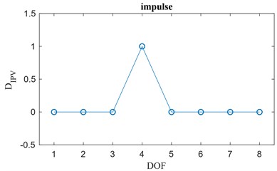
Depending on the structural boundary conditions (structural constrains) and material properties, the damage index vector can present different types of jump discontinuity and so a local damage index vector can be defined based on the type of jump discontinuity presented in the plot of the damage index vector. Three possible cases are here reported, considering the way that the structural damage affects the mechanical characteristics of the structure:
1. If all the DOFs but the closest to the damage location are more sensitive to the structural constrains than to the occurrence of damage, the damage index is approximatively null at those locations away from the damaged one. Fig. 1(a) shows a possible configuration plot of the damage index vector for the case in which, by considering a local damage between DOFs 3 and 4, only the 4th element of shows an appreciable variation (in this specific case, it is arbitrarily set equal to 1 to provide a clear graphical representation). The plot of the damage index vector is similar to one representing an impulse change. For such a specific case, the local damage index is defined as the damage index vector itself so that .
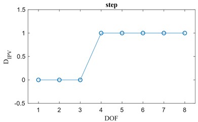
2. It might happen that, for specific boundary conditions and material properties, the presence of a local damage may induce a step change as jump discontinuity in the trend of the plotted elements of the damage index vector. An example is shown in Fig. 1(b) where the two trends are represented by arbitrarily setting the elements of the vector to zeros and ones. Again, the damage has been introduced between the DOFs 3 and 4. In this case, the local damage index vector is provided by the first order difference of the damage index vector, . The elements of related to the position halfway between two adjacent monitored positions and are given by:
where the index of the element indicates the location halfway between the th and th elements of the vector indicated by and . In this particular case so that . In this case, the local damage index vector is defined as .
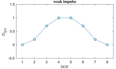
3. Finally, for some boundary conditions and material properties, it is possible that all the elements of the damage index vector are sensitive to the local damage, and their plot looks like a weak impulse. This is the case depicted by Fig. 1(c) in which a damage between the DOFs 4 and 5 is represented. For this particular case to locate the damaged area, the local damage index vector can be defined as the second order difference of the damage index vector, . The elements of the vector are computed as follows:
for setting, for convenience, so that .
Fig. 1a) Impulse change, b) step change, c) weak change
a)
b)
c)
In summary, Fig. 1 represents the three abrupt changes in the damage index vector, each of which is related to particular structural cases. For each of them it is possible to derive a local damage index vector linked to the change of the damage index vector: this operation is usually performed manually, but classification algorithms that rely on cross-correlation or classifiers can be designed in order to automate such process.
The final goal of this damage assessment algorithm is to detect abrupt changes in the elements of the local damage index vector to assess the presence of locations of potential damage. In order to quantify the entity of these abrupt changes, the introduction of a threshold value for the elements of the local damage index vector is necessary, as shown in the next section.
2.4. Damage threshold for the local damage index vector
The most suitable approach for the definition of a threshold for local damage index vector is the one proposed by Wang et al. [6, 20] based on the statistics (mean and the standard deviation) of the elements of such a vector. The upper and lower threshold boundaries, and , are defined as:
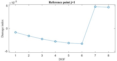
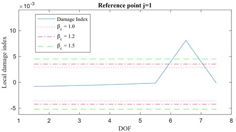
where and are respectively the mean and the standard deviation of the local damage index vector . The term is a constant value set to define a confidence interval and is commonly assumed to be . For instance, in case of normal distribution of the values of the elements of the local damage index vector, the choice of , and leads to a confidence interval respectively of 76.99 %, 86.64 % and 92.81 %. When the threshold is overcome by some values of the elements of the local damage index vector, the structure is claimed to be damaged and the location of the local damage is detected. A brief example is reported in Fig. 2.
Fig. 2a) Damage index vector {DIPV,j,r'} classified as step change and b) local damage index vector {LIPV,j,r'}
a)
b)
Let’s focus, for instance, on an 8-DOF system whose damaged state is characterized by a localized damage between the DOFs 6 and 7. By looking at Fig. 2 (a) the damage index vector for and can be easily classified in the step change class (Fig. 1(b)) while the corresponding local damage index vector , is plotted in Fig. 2(b). Also, in Fig. 2(b), the thresholds are shown for , and . It is evident that the plot of the local damage index vector indicates that damage has occurred between the DOFs 6 and 7.
3. The IPV in an output-only framework
The effectiveness of the IPV algorithm has been exhaustively proven by Wang et al. In their study [6] they analyzed a lumped element mock up excited by a low-pass (LP) filtered input: this input was designed so to excite exclusively the first natural frequency of the undamaged system. Obviously, this step requires a preliminary laboratory test in order to identify the natural frequencies of the system. After recording the acceleration response time histories for the system in undamaged conditions, local damage was introduced in the structure and, using a band-passed input with the same cut-off frequencies as the one used in the undamaged structure, the acceleration response of the frame in damaged conditions was recorded. By applying the IPV theory based on the cross-correlation of the signals for the undamaged and damaged states, the algorithm accurately identified the location of the damage (IPV in Fig. 3).
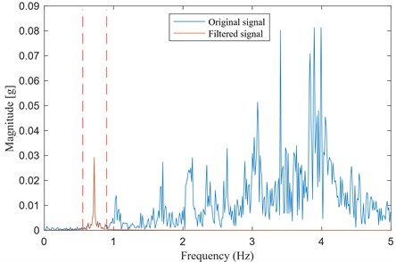
As mentioned, the condition of a properly designed band-pass (BP) filtered signal to induce a specific system excitation is a valid option for laboratory tests only: it implies that the structure be subjected to two tests, one to determine the frequency range of interest and the other to collect data to be used in the identification of the IPV. In the methodology presented in this paper, only one test is required. In fact, instead of filtering the input excitation, it is proposed that the filtering procedure be performed on the acceleration response time histories from the only test. Such a filtering procedure is allowed as long as all the theoretical assumptions at the base of the proposed methodology (e.g. richness and independence of the input forces) are respected. Hence, the approach presented in this paper will then be referred to as output-only IPV (Fig. 4): it allows us select the response contribution of the th structural mode to be isolated and examine it directly from the spectrum of the response output. After the selected component of the acceleration response has been isolated, the IPV method can be applied to obtain the local damage index vector.
Fig. 3IPV (Wang et al.)
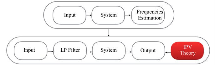
Fig. 4Output-only IPV (filtered output)

The proposed methodology has some advantages with respect to the original IPV-based approach [6] and to the conventional parametric system identification based approaches (e.g. Output-Only Observer Kalman filter [17], Stochastic Subspace Identification [18], etc.) for damage assessment purposes. This method extends the boundaries of the original IPV approach by allowing an output-only analysis using information from higher modes than the first one. The possibility of using multiple reference points allows us to indirectly extract information about the analyzed structural mode shape by looking at the characteristics of the identified IPVs. Another main advantage of the proposed method is its easiness in handling large datasets from dense sensor networks: traditional identification methods rely on regression models and might suffer from the curse of dimensionality when dealing with large covariance matrices. Instead, the calculations associated with the cross-correlation vectors for the IPVs are much more efficient in terms of computational efforts. However, there are also some drawbacks in the proposed methodology: the main one is the undesired contribution of other structural modes that can be difficult to be filtered out from the one considered and may induce undesired noise effects.
4. Analysis of the results
To evaluate the performance of the proposed output-only IPV method in assessing and locating structural damage, numerical simulations as well as experimental data have been considered.
4.1. Numerical simulation: 8-DOF lumped model
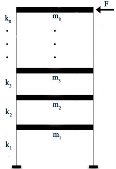
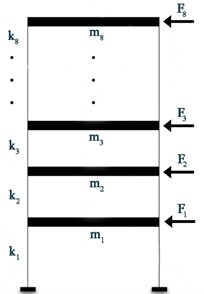
The model of the structure is an 8-DOF shear-type model matching the one employed by [11] and is shown in Fig. 5(a). In its baseline undamaged conditions, the system is characterized by springs of stiffness N/m and masses kg for . The frame is characterized by modal damping with a damping factor of 1 % for each of the 8 vibration modes. The force excitation is applied horizontally on the 8-DOF model via zero-order-hold (ZOH) with a time sampling of 0.01 seconds: it is a zero-mean Gaussian signal with standard deviation N and is applied at the top of the model (Fig. 5(a)). The input/output time histories are 100 seconds long leading to 10,000 time steps for each signal. In order to simulate a local damage, the 8-DOF system has been weakened by decreasing the stiffness of the spring between the 4th and 5th floors by 20 %.
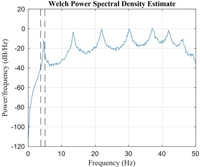
Once the acceleration response time histories have been simulated, a spectral analysis can be carried out in order to select a suitable mode to be investigated. In this first example, in order to show the effectiveness of the proposed approach, let us assume that there is no measurement noise in the response signals (it will be included at a later stage).
Fig. 5a) 8-DOF shear type system, b) spectral analysis for the 1st floor: power spectral density
a)
b)
In this case, all the modes appear to be well excited and separated, thus we can select one of them and filter out the contributions of the other modes. It is noteworthy to point out that generally, for civil engineering applications, e.g. buildings, it is common practice to explore lower frequencies rather than the higher ones because they have better resolution and they are more easily excited. Therefore, the proposed algorithm is applied to data obtained by considering only the contribution of the first mode. Based on the spectral analysis, the lower and upper cut-off frequencies of the band pass filter have been set to 4.3 Hz and 5 Hz respectively (see Fig. 5 (b)).
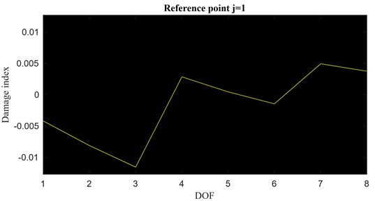
In the proposed methodology, the computation of the IPVs (Eq. (12)) and, consequently, of the damage index (Eq. (14)) requires the selection of an arbitrary th reference point. The components of the damage index vector for any choice of the reference point are reported in Fig. 6.
Fig. 6Damage index vector for j=1,2,…, 8 as defined in Eq. (14), r'=1
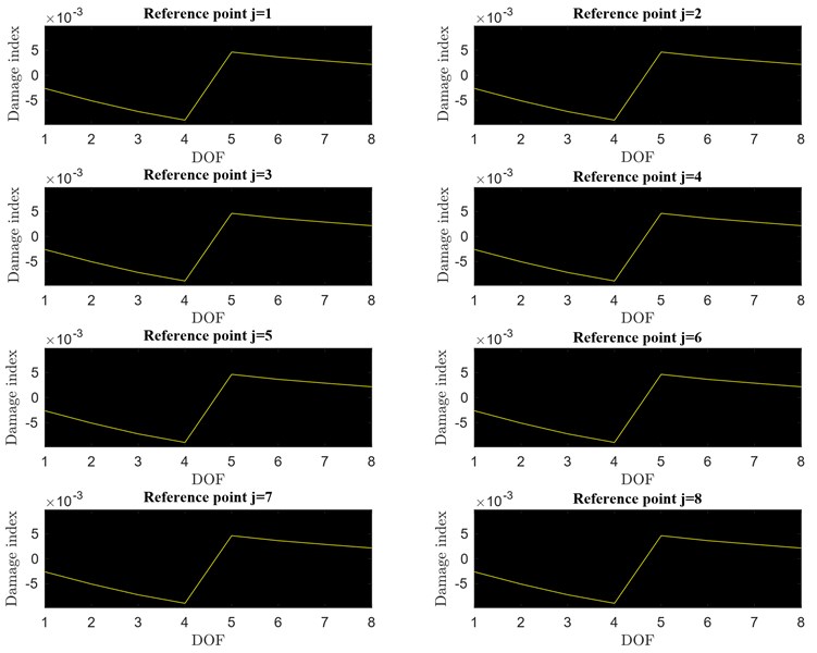
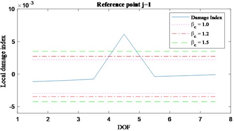
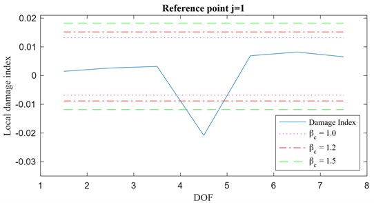
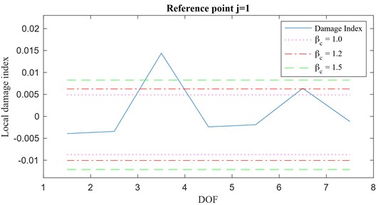
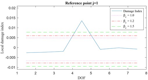
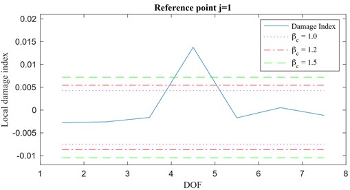
Looking at Fig. 6, it can be concluded that, no matter what th reference position is selected, the damage index vector always shows a jump discontinuity between the lumped elements bounding the damaged spring. Such kind of discontinuity let the damage index vector be classified into the step change class (Fig. 1(b)). Thus, the elements of the local damage index vector can be obtained using Eq. (23). The local damage index vector for 1 is plotted over the monitored DOFs in Fig. 7(b) with the threshold set for three different values of (1.0, 1.2 and 1.5). Clearly, from the analysis of the results, it appears that the proposed algorithm is successful in detecting the damage between the 4th and 5th floors for any of the three values of . Fig. 7(a) shows an analogous result for a damage simulated by 10 % drop in stiffness between the DOFs 4 and 5.
These numerical simulations based on an output-only approach can be compared with those obtained following the approach by Wang et al. [6] which rely on input-output information. By considering this noise free experiment, a band pass filter applied to the acceleration response time histories leads to the same results obtained by filtering the excitation source. It is worthy to recall that, in this specific case, the frequency contribution provided by modes other than the first one () have been considered negligible in the filtered frequency band. Of course, this condition implies that the natural frequencies related to those neglected modes should be far enough from the one of the analyzed mode or, at least, the contribution of those modes to the total response should not be significant in the vicinity of such a frequency.
Fig. 7Local damage index vector, a) 10 % damage, b) 20 % damage, r'=1
a)
b)
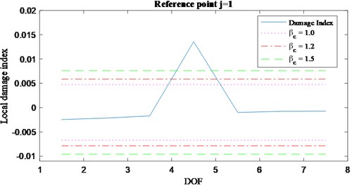
Fig. 8Damage index vector for j=1,2,…, 8 ad defined in Eq. (14), r'=2
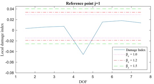
As the spectral analysis suggests, also the mode related to the second peak appearing in Fig. 5(b) () can be isolated and used in the estimation of the IPVs taking advantage of the flexibility of the proposed methodology. For this purpose, the lower and upper cut-off frequencies of the Finite Impulse Response (FIR) filter have been set equal to 13 Hz and 14.5 Hz respectively. Again, the damage index vector is computed for any reference point and such vectors are presented in Fig. 8. A jump discontinuity, similar to the one already shown in Fig. 6, appears between the DOFs 4 and 5, revealing the presence of damage. However, an interesting observation can be made by looking at the plots in Fig. 8: it appears that the damage index vectors computed for are ’mirror’ images of those obtained for . The reason why two different types of damage index vectors appear is due to the fact that, recalling Eq. (14), the sign of the damage index vector depends on the sign of the component of the mode in question at the th reference location (). Thus, moving from the reference point to the reference point , the damage index changes its sign because there is a sign change between the 5th and 6th components of the second mode. Since this is a peculiarity of the mode analyzed (in this case the second), it can be concluded that the damage index vectors also provide information about the selected mode shape.
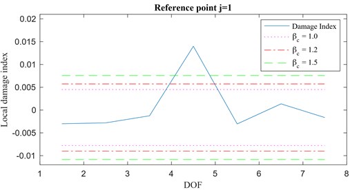
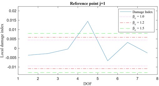
Analogously to the previous analysis (), also in this case the damage index vector is claimed to belong to the class defined as a step change and the local damage index vector (for ) is shown in Fig. 9 for a drop in stiffness of the 10 % (a) and for a drop in stiffness of the 20 % (b).
Fig. 9Local damage index vector, a) 10 % damage, b) 20 % damage, r'=2
a)
b)
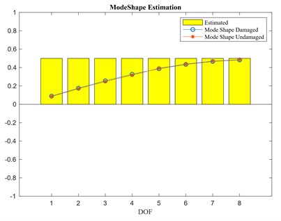
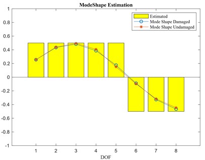
To show the effect of the sign of the component of the selected mode at the reference location on the damage index vector, the sign of the first two mode shapes ( and ) for reference locations is shown in Fig. 10 together with the corresponding mode shapes. The bars, providing an estimate of given by changes in the sign of the damage index vector , have been arbitrarily set equal to +0.5 when is positive and equal to -0.5 when it is negative. According to Fig. 6, for the damage index vector never changes its sign over different reference locations since the components of the first mode have all the same sign (Fig. 10(a)). On the contrary, looking at Fig. 8, the damage index vector obtained for changes its sign moving from the reference location to , in agreement with the second mode shape (for both damaged and undamaged conditions).
Fig. 10a) First mode shape estimation, b) second mode shape estimation
a)
b)
Fig. 11a) Double local damage: damage index vector, b) local damage index vector (for step change)
a)
b)
It is important to mention that, even in the case of multiple damage locations, the proposed methodology is successful in locating the damaged areas. Fig. 11 shows the damage index vector and the corresponding local damage index vector for a double damage occurrence between the DOFs 3 and 4 and the DOFs 6 and 7.
Finally, it should be remarked that, as long as the single mode’s contribution to the acceleration responses can be isolated, the normalization in Eq. (11) removes any effect of the input. Consequently, any change in the position and/or magnitude of the input from the undamaged to the damaged configuration doesn’t affect the final solution. This is one of the advantages of the proposed methodology because tests are generally performed under different excitation configurations and so removing the requirement of identical testing conditions from the undamaged and damaged tests free engineers from unnecessary constrains.
4.2. Fully excited system: effects of measurement noise
To look at the impact of external disturbances on the accuracy of the results, let’s consider the same 8-DOF shear-type system subjected to an external excitation at every DOF. Each input force is represented by a zero-mean Gaussian white noise signal, with standard deviation of 1 N, and it is uncorrelated with the others. The disturbance representing measurement noise has been modelled as an additional zero-mean white noise signal, having a root mean square (RMS) equal to a certain percentage of the RMS of the output, and added to the output signals. Because of the stochastic nature of the external white noise excitation, a statistical approach based on Monte Carlo simulations has been used to highlight the effect of noise disturbances on the damage index vector.
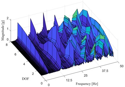
Fig. 12a) Excitation setup, b) waterfall plot
a)
b)
The baseline configuration of the structure and the excitation setup are shown in Fig. 12(a), whereas the waterfall plot of the magnitude of the spectrum of the acceleration time histories, at each DOF, is presented in Fig. 12(b). Also, in this case, the first mode () seems to be the perfect candidate for the structural damage assessment through the proposed methodology. Through Monte Carlo simulations, 50 realizations of the cross-correlation vectors and have been generated in order to obtain the damage index vector . Damage has been simulated by introducing a 20 % stiffness reduction between the DOFs 4 and 5. Local damage index vectors for a noise with RMS of 1 %, 5 %, 10 % and 20 % are reported in Fig. 13. These plots show that, as long as the assumptions behind of the theory of the IPV are fully respected, the damage index shows a remarkable robustness to white noise disturbances and remains a good indicator of damaged areas.
Fig. 13Local damage index vector for varying RMS of noise: a) 1 %, b) 5 %, c) 10 %, d) 20 %
a)
b)
c)
d)
4.3. Numerical simulation: 100 DOF model
This section extends the investigation about the applicability of the proposed IPV-based damage index vector to a more complex system, (e.g. a plate) represented by a two-dimensional frame (Fig. 14(a)). The structure is a 2-D square grid of 10×10 lumped masses of 1 kg each connected by spring elements placed horizontally, vertically and diagonally, each one having stiffness of 1000 N/m, 900 N/m and 800 N/m respectively. The modal damping has been set to 1 % for all vibration modes. The structure is doubly-fixed at the top and at the bottom and a set of excitation forces acts perpendicular to the plane of structure. Using the assumption of zero-order-hold (ZOH) with a time sampling of 0.01 seconds, these forces are represented by zero-mean Gaussian signals (uncorrelated to each other) with standard deviation of 1 N and a length of 100 seconds.
Fig. 14a) 100 DOF mock up, b) spectrum
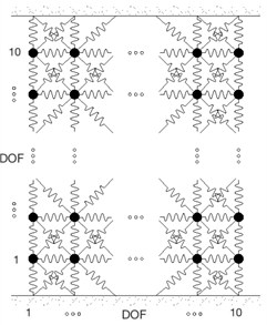
a)
b)
Fig. 14(b) shows the spectral magnitude of the response of the system at DOF 50, i.e. 5th row from the bottom, 10th column from left of the model shown in Fig. 14(a). The spectral analysis suggests that the first mode contribution is the most suitable to be analyzed through the proposed IPV-based approach since it appears well isolated by the other structural modes (0.72 Hz).
Fig. 15a) Simulated damage spot, damage index vector, b) 2-D representation
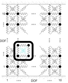
a)
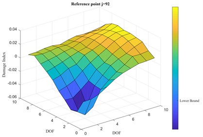
b)
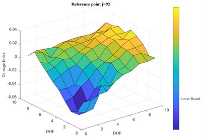
The damage is simulated through a drop in stiffness of 25 % for two of the diagonal springs, as shown in Fig. 15(a). After checking that the damage index vector for each th reference point of the 100 DOFs is consistent with the others, Fig. 15 (b) shows the value of the computed damage index vector for a randomly picked reference point 92, i.e. 10th row from the bottom, 2nd column from left, far from the damage location. It is clear that the damage location can be identified by just looking at the plot of the damage index vector . The threshold for the damage has been set accordingly to the mean and the standard deviation of the elements of the damage index vector so that, for a value of the standard deviation multiplier 1.8, the ’Upper Bound’ is set at 0.0334 and the ’Lower Bound’ at –0.0356. The latter is reported in the colorbar of Fig. 15(b).
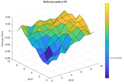
Increasing the level of measurement noise in the response output signals to 5 % RMS and 10 % RMS does not prevent the proposed IPV-based approach to find the damage location, as seen in Fig. 16. In this case, the corresponding ’Upper Bound’ and ’Lower Bound’ are respectively 0.0347 and –0.0375, for the case in Fig. 16(a), and 0.0362 and –0.0387, for the case in Fig. 16(b).
These numerical tests confirm the effectiveness of the proposed IPV-based methodology for damage identification and localization even in the case x more complicated structural models.
Fig. 16Damage index vector, 2-D representation: a) 5 % RMS, b) 10 % RMS
a)
b)
5. Experimental test: LANL 3-DOF shear-type
The proposed approach has also been tested on experimental test results obtained from a 3-DOF shear-type system shown in Fig. 17(a). Test data have been provided by the Engineering Institute (EI) at Los Alamos National Laboratory (LANL) [19-21]. The system consists of four aluminum columns (17.7×2.5×0.6 cm) connected at the top and bottom to aluminum plates 30.5×30.5×2.5 (cm) [22], forming a structure consisting of 3 floors and a sliding base. The excitation is provided by an electromagnetic shaker that acts at the center line of the base floor of the structure. Both the structure and the shaker are fixed on a base plate (76.2×30.5×2.5 cm). Four accelerometers with a nominal sensitivity of 1000 mV/g are attached at the center of the side of each floor at the opposite side from shaker to measure the response of each plate. The random excitation applied at the sliding base is band limited in the range of 20-150 Hz to avoid rigid body modes of the structure. Even if the structure was initially supposed to behave linearly, some non-linear effects due to the sliding rails have been noted [23].
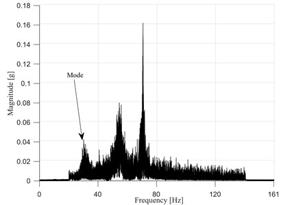
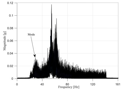
Fig. 17(b) shows the magnitude of the output response spectrum computed through Fast Fourier Transform (FFT) for each floor in undamaged conditions. From previous studies [21], the natural frequency of the first mode has been determined to be 30.7 Hz. However, the information obtained through the FFT shows that such a natural frequency is not well excited at the 2nd and 3rd floors by the selected input.
The LANL database supplies data about force and accelerations recorded for three different structural conditions (different damage scenarios), other than the original (baseline or healthy) condition. The three damage conditions have been imposed through stiffness reduction of the columns connecting the floors. The damage scenarios considered in this dataset are the following:
– 50 % stiffness reduction between floors 1-2.
– 50 % stiffness reduction between floors 2-3.
– 50 % stiffness reduction between floors 3-4.
Fig. 17a) LANL 3-DOF shear-type, b) channels 2-5 FFT magnitude
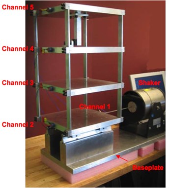
a)
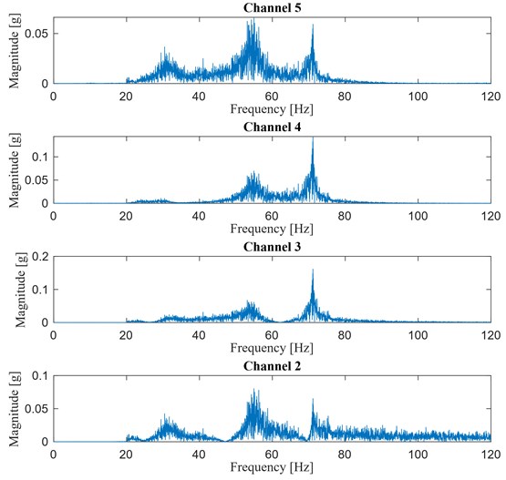
b)
Since the sliding plate (floor 1) can move along the sliding rails when subjected to the shaker action, such a motion will be considered as an additional DOF (DOF 1) so that the model can be analyzed as a 4-DOF system.
5.1. 50 % stiffness reduction between floors 1-2 and 2-3
As previously done, the first step is the spectral analysis of the output response in order to evaluate the contribution of the various modes for both the damaged and undamaged configurations. The magnitude of the spectral response of the system in the undamaged and damaged configuration for damage case 1 is shown in Fig. 18 where the spectra of the structural accelerations at each DOF are superimposed. It appears that, after the occurrence of damage, a huge drop of the stiffness between floors 1-2 induces the first natural frequency to shift of almost 2 Hz. For such a reason, a band pass filter with cut-off frequencies at 29 and 33 Hz has been adopted in undamaged conditions whereas in damaged configuration the cut-off frequencies have been changed to 27 and 31 Hz.
Fig. 182-D representation of the Magnitude of the spectral response in a waterfall plot: a) undamaged structure, b) damaged structure, damage between floors 1-2
a)
b)
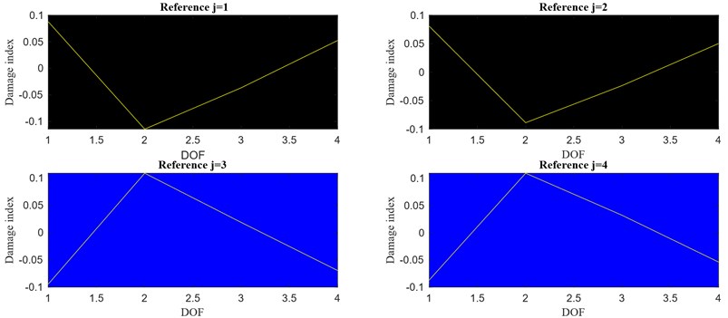
Fig. 19 shows the plots of the calculated damage index vector as function of the DOFs for different th reference points ( 1,…, 4). As seen in the numerical example, when moving from reference point 2 to 3, the values of the damage index change sign because of the sign change between the two corresponding modal components in Eq. (14). This indicates that the mode considered in the damage assessment analysis is not the first mode: this would have prevented the application of the original formulations of the IPV based approach (Wang et al. [6]). However, this obstacle has been overcome with the proposed methodology.
Fig. 19Damage index vector over different reference points
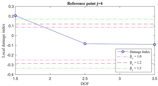
Usually the threshold for the damage localization relies on calculations of the mean and standard deviation of the elements of the local damage index vector: however, monitoring only 4 positions, the damage index vector contains 4 values only (i.e. Fig. 19) and its first derivative (representing the local damage index vector) only 3 (i.e. Fig. 20). Hence, finding outliers among just 3 points can be difficult when using only mean and standard deviation. However, in this case, having only 3 points does not seem to be a limiting factor: in fact, even with just points, the algorithm is capable to locate the damaged columns as shown in Fig. 20(a) for case 1 (damage between DOF 1 and DOF 2) and in Fig. 20(b) for case 2 (damage between DOF 2 and DOF 3).
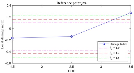
Fig. 20Local damage index vector for a) case 1 and b) for case 2. Reference point j= 4
a)
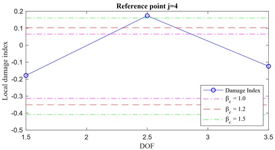
b)
5.1.1. 50 % stiffness reduction between floors 3-4
In this case, even though the analysis of this damage scenario is conducted along the same line as the previous ones, something different happens. As shown in Fig. 21, where the damage index vectors for 1, 2, 3, 4 are plotted, an interesting behaviour is shown for the case of reference point 3 with the corresponding damage index vector showing an inconsistent pattern with respect to the other vectors.
As discussed in [24], the imaginary part of the Frequency Response Function (FRF) provides information about the shape of a particular mode. In Fig. 22, the imaginary part of the response spectra in the frequency range in which the signal is filtered is plotted over the DOFs for the undamaged (a) and damaged (b) conditions. It can be noted that passing from the former (undamaged) to the latter (damaged), the imaginary part for the FRF for DOF 3 changes its sign (from negative -undamaged- to positive -damaged-) violating the theoretical assumption allowing to pass from Eq. (13) to Eq. (14). As a consequence, the reference point 3 does not constitute a reliable reference point. All the other DOFs ( 1, 2, 4) are valid reference points, leading to the correct solution.
Using the damage index vectors in Fig. 22, it is possible to compute the corresponding local damage index vector and successfully locate the damaged area, Fig. 23(a).
It is interesting to observe that, for this particular study case, the presence of a rigid body mode does not allow to use the mode related to the first natural frequency of the system in the calculation of the IPVs. Since the first mode has a very low natural frequency, its contribution is mixed with that of the rigid body mode and a low pass filter (0-20 Hz) applied to the input excitation helps removing such a contribution in the original acceleration response time histories. This would impair the use of the original formulation of the IPV approach presented by Wang et al. [6]; instead, it does not represent a problem for the current formulation because of its ability to handle higher modes. In addition, the next mode, the one with the lowest natural frequency in the spectrum, presents a structural node at the third floor for the structure in damaged condition (damage between DOFs 3 and 4) and so the arbitrary selection of the reference point might lead to some numerical inaccuracies (Fig. 21, Reference 3). It is then recommended, when using the proposed methodology, to compute the damage index vector for multiple reference points in order to verify their compatibility and correctly assess the presence of local damage.
Fig. 21Damage index vector over different reference points
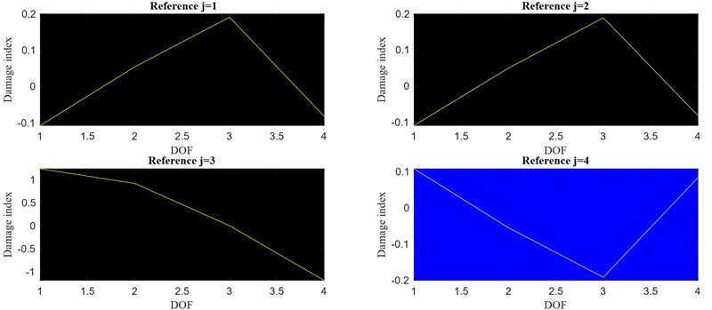
Fig. 22FRF, imaginary part. a) Undamaged configuration, b) damaged configuration
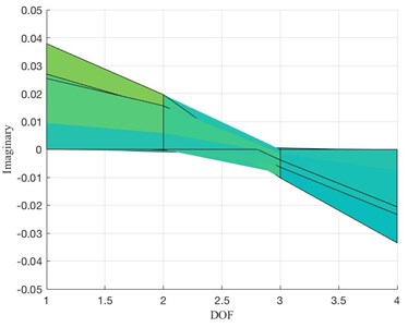
a)
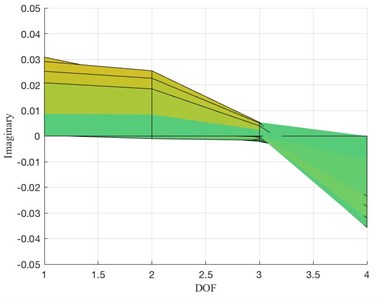
b)
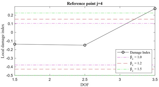
Finally, as a further validation of the effectiveness of the proposed method in assessing the damage location, the case of a unit pulse excitation is analyzed. Considering the acceleration response time histories for case 3 (damage between floors 3-4), the unit pulse response can be obtained by considering the Markov parameters extracted through an input-output identification algorithm, e.g. Observer Kalman Identification [23, 25]. By using the system’s Markov parameters sequences as unit pulse responses into the proposed IPV-based methodology, it is possible to obtain the corresponding local damage index vector. A comparison between the local damage index vectors obtained using a Gaussian white noise excitation (a) and a unit pulse response (b) is shown in Fig. 23. The results are consistent and a successful damage localization is achieved.
Fig. 23Local damage index vectors for a) white noise and b) unit pulse excitation
a)
b)
6. Conclusions
In this paper, a new formulation of a IPV based approach to damage detection is proposed. Differently from the original IPV formulation, this methodology relies on information extracted only from the dynamic response of the structure, without knowledge of the input excitation, e.g. in an output-only context. With respect to the original input-output formulation, there is no need to design an input excitation that is properly tailored to the structural characteristics, reducing the number of necessary tests. In addition, the proposed methodology allows for the analysis of higher modal contributions, eliminating the constrain to account only for the first mode as in the original formulation. The only requirement is the design of a band-pass filter needed to extract the energy contribution of a specific mode in the structural response. The validity of the proposed output-only IPV based theory has been proven for unit impulse and white noise excitations. Numerical simulations on small and large system models as well as experimental data analyses have confirmed the effectiveness of the methodology.
From an engineering point of view, the proposed methodology has many advantages with respect to both the original input-output formulation and the conventional system identification damage assessment strategies. Compared with the original IPV based formulation, the proposed approach requires fewer tests since it does not need a preliminary test to properly design a filter to extract the first mode contribution from the dynamic response. Furthermore, the analysis of structural modes other than the first one extends the applicability of the methodology to more general laboratory test investigations where it is difficult to excite and correctly extract low frequency modal contributions. Another major advantage of the proposed methodology is its ability to handle datasets from large sensor networks: when using system identification methods for structural damage assessment, large datasets might lead to huge computation efforts that result in inaccurate estimations of the damage and its locations. Contrarily, the proposed approach can easily handle large dataset since the estimation of the cross correlations between filtered responses of the system requires much less computation than the estimation of the covariance matrices. Hence, because of its capabilities to handle large sensor networks, the resolution of the damage assessment and localization increases.
References
-
Sohn H., Farrar C. R., Hemez F. M., Shunk D. D., Stinemates D. W., Nadler B. R., Czarnecki J. J. A Review of Structural Health Monitoring Literature: 1996-2001. Los Alamos National Laboratory, USA, 2003.
-
Worden K., Manson G., Fieller N. Damage detection using outlier analysis. Journal of Sound and Vibration, Vol. 229, Issue 3, 2000, p. 647-667.
-
Worden K., Farrar C. R., Manson G., Park G. The fundamental axioms of structural health monitoring. Proceedings of the Royal Society A: Mathematical, Physical and Engineering Sciences, Vol. 463, Issue 2082, 2007, p. 1639-1664.
-
Sohn H., Allen D. W., Worden K., Farrar C. R. Structural damage classification using extreme value statistics. Journal of Dynamic Systems, Measurement, and Control, Vol. 127, Issue 1, 2005, p. 125-132.
-
Balsamo L., Betti R. Data-based structural health monitoring using small training data sets. Structural Control and Health Monitoring, Vol. 22, Issue 10, 2015, p. 1240-1264.
-
Wang L., Yang Z., Waters T. P., Zhang M. Theory of inner product vector and its application to multiple-location damage detection. Journal of Physics: Conference Series, Vol. 305, Issue 1, 2011, p. 012003.
-
Wang S., Ren Q., Quiao P. Structure damage detection using local damage factor. Journal of Vibration and Control, Vol. 12, Issue 9, 2006, p. 955-973.
-
Trendafilova I., Manoach E. Vibration-based damage detection in plates by using time series analysis. Mechanical Systems and Signal Processing, Vol. 22, Issue 5, 2008, p. 1092-1106.
-
Kim J., Stubbs N. Crack detection in beam-type structures using frequency data. Journal of Sound and Vibration, Vol. 259, Issue 1, 2003, p. 145-160.
-
Wang L., Yang Z. C. Structural damage detection using inner product vector and low pass filter technique. Applied Mechanics and Materials, Vol. 204, 2012, p. 2942-2946.
-
Zhang M., Schmidt R., Markert B. Structural damage detection methods based on the correlation functions. Eurodyn, 2014.
-
Roy K., Ray Chaudhuri S. Fundamental mode shape and its derivatives in structural damage location. Journal of Sound and Vibration, Vol. 332, Issue 21, 2013, p. 5584-5593.
-
Iezzi F., Spina D., Valente C. Damage assessment through changes in mode shapes due to non-proportional damping. Journal of Physics: Conference Series, Vol. 628, Issue 1, 2015, p. 012019.
-
Salawu O. Detection of structural damage through changes in frequency: a review. Engineering structures, Vol. 19, Issue 9, 1997, p. 718-723.
-
Doebling S. W., Farrar C. R., Prime M. B., Shevitz D. W. Damage Identification and Health Monitoring of Structural and Mechanical Systems from Changes in Their Vibration Characteristics: a Literature Review. Los Alamos National Lab., NM (United States), Tech. Rep., 1996.
-
Dawari V., Vesmawala G. Structural damage identification using modal curvature differences. IOSR Journal of Mechanical and Civil Engineering, Vol. 4, 2013, p. 33-38.
-
Vicario F., Phan M. Q., Betti R., Longman R. W. Output-only observer/Kalman filter identification (O ^3KID). Structural Control and Health Monitoring, Vol. 22, Issue 5, 2015, p. 847-872.
-
Brinker R., Andersen P. Understanding stochastic subspace identification. Proceedings of the 24th IMAC, St. Louis, Vol. 126, 2006.
-
Figueiredo E., Flynn E. Three-Story Building Structure to Detect Nonlinear Effects. Report SHMTools data description, Los Alamos National Laboratory, 2009.
-
Hernandez Garcia M.-R., Masri S. F., Ghanem R., Figueiredo E., Farrar C. R. An experimental investigation of change detection in uncertain chain-like systems. Journal of Sound and Vibration, Vol. 329, Issue 12, 2010, p. 2395-2409.
-
Figueiredo E., Park G., Figueiras J., Farrar C., Worden K. Structural Health Monitoring Algorithm Comparisons Using Standard Data Sets. Los Alamos National Lab. (LANL), Los Alamos, NM (United States), Tech. Rep., 2009.
-
Hernandez Garcia M.-R., Masri S. F., Ghanem R., Figueiredo E., Farrar C. R. A structural decomposition approach for detecting, locating, and quantifying nonlinearities in chain-like systems. Structural Control and Health Monitoring, Vol. 17, Issue 7, 2010, p. 761-777.
-
Vicario F. Okid as a General Approach to Linear and Bilinear System Identification. Ph.D. dissertation, Columbia University, 2014.
-
Avitabile P. Experimental modal analysis (a simple non-mathematical presentation). Sound and Vibration, Vol. 35, Issue 1, 2001, p. 20-31.
-
Vicario F., Phan M. Q., Betti R., R. W. Longman Okid as a unified approach to system identification. Advances in the Astronautical Sciences, Vol. 152, 2014, p. 3443-3460.
Cited by
About this article

