Abstract
Cracks and other damages generated during the service of bridges can reduce the load bearing capacity and threaten operational safety.Finite Element Model Updating (FEMU), as one of the important means of structural health diagnosis, identifies structural damage through changes in model parameters. The three key factors of FEMU are updating variables, objective functions, and optimization algorithms. The poor selection of the above three factors in existing research leads to high calculation errors in model updating, and inevitably lead to the inability of the finite element model to carry out structural health monitoring, affecting the normal operation of the structure. In order to solve the above problems, this paper combines previous research and establishes a model updating algorithm based on the combination of eigenvector difference approach and particle swarm optimization (ED-PSO). The validity and accuracy of this method are verified by finite element analysis of a simply supported beam. Compared with the existing model updating algorithms based on the combination of static and dynamic methods and particle swarm optimization (CSD-PSO), the results show that the proposed ED-PSO model updating algorithm has higher accuracy and is expected to be better applied to bridge finite element model updating research.
1. Introduction
As an important component of transportation infrastructure, bridges are the key to the normal operation of the transportation system [1]. Once a bridge structure is damaged, there will be structural damage, collapse, and other phenomena, seriously endangering the safety of society and people's lives and property. There are various reasons for bridge accidents, among which inadequate structural health monitoring of bridge structures is the main reason [2]. Damage identification is one of the main challenges in bridge health monitoring. It can help assess the safety status of bridges, prevent catastrophic collapse, and provide relevant maintenance information [3]. Accurate finite element models are essential for accurate structural damage detection. However, there is uncertainty in the structural model and measurement response of actual structures, and the model parameters are random, so this randomness leads to uncertainty in the analysis results. For bridge structures, during operation, factors such as performance degradation of components and section failure may deviate from design parameters (such as section size, density, modulus of elasticity, etc.). This leads to a deviation from the actual structure when establishing a finite element model [4]-[5]. Therefore, in order to obtain an accurate finite element model, it is necessary to update the relevant parameters of the finite element model.
The essence of finite element model updating is an optimization problem. The process of constructing a corresponding objective function with relevant parameters that minimize system response, minimizing the value of the objective function through optimization processing, and updating the initial finite element model of the dynamic system to minimize the difference between it and actual model predictions [6]. Thereby gradually bringing the response of the finite element model closer to the real structure for structural health detection [7]. Currently, there has been a lot of research on finite element model updating. Carvalho [8] et al. have successfully applied the optimal matrix method model updating technology to model updating of incomplete measured modal data. Wang [9] et al. obtained good updating results by updating the model of a bridge and using the elastic modulus of concrete and steel bars of the bridge as updating parameters.Guvenc Canbaloglu [10] et al. completed model updating of nonlinear structures by testing the frequency response function of nonlinear structures, and achieved good results. Paya Zaforteza [11]et al. used simulated annealing algorithms to update the model of a reinforced concrete frame. Banan M. R. and Hjelmstad K. D. [12] estimated the element stiffness through testing to static displacement, and proposed a model updating method with relatively few parameters. Collins [13] et al. successfully updated various physical parameters of the finite element model by using the residual between the measured modal response values of the structure and the modal response values calculated by the finite element model as the objective function. Brownjohn [14]et al. used finite element model updating based on parametric methods to identify structural dynamic characteristics and evaluate structures of highway bridges. Cao [15] et al. proposed a time domain response model updating method based on dynamic sensitivity. Using a cantilever beam numerical model, it was verified that this method has good noise resistance performance and can obtain high-precision nonlinear dynamic response prediction numerical models. Mottershead [16] et al. conducted a comprehensive and systematic discussion on various sensitivity based model updating methods and demonstrated their application effects on Lynx helicopters. The work also includes the use of special updating parameters, such as compensation nodes and generic elements. Gorl and Link [17]updated the theoretical model based on the experimental data of the initial model and the damage model, respectively, and then extracted the damage parameters of the steel frame as a benchmark. Sarvi [18] et al. demonstrated the specific performance of usage of the enhanced Levenberg-Marquardt algorithm, which is designed for nonlinear least squares problems in the updating process. Moaveni [19] et al. applied model updating methods to detect damage in reinforced concrete frames filled with volume.
From a practical perspective, the realization of finite element model updating technology is challenging, with the main difficulties reflected in how to construct the objective function, select the variables to be updated, and select optimization algorithms. The above factors directly determine the quality of the finite element model updating work [20]-[21].
Currently, particle swarm optimization (PSO) algorithms have been widely used in the research of solving optimization problems. PSO algorithms have the characteristics of fast convergence speed and high accuracy in solving optimal values. However, the combination of PSO algorithms and objective functions to achieve good model updating calculation results is the focus of current research. Maosen Cao [22] et al. used particle swarm optimization algorithm to identify the damage of a layered fixed beam at both ends, and accurately identified the damage of the beam structure through different delamination. Zhang [23]et al. used particle swarm optimization to update the geotechnical structure model, and also obtained relatively accurate updating results. Lin [24]et al. applied particle swarm optimization algorithms to estimate the parameters of nonlinear dynamic rational filters. Kathiravan and Ganguli[25] used particle swarm optimization algorithms to design the optimal layup of composite box girder structures that can be used as the main load-bearing components of helicopter rotor blades. Seyedpoor [26]proposed a two-stage damage detection method, in which the particle swarm optimization algorithm is used in the second stage to evaluate the degree of damage based on measured values of vibration modes. The work of Liu [27] et al. is to apply particle swarm optimization algorithm to the parameter identification problem of permanent magnet synchronous engines. Perez and Behdinan [28] improved the basic particle swarm optimization algorithm for constrained structure optimization problems. Hassan [29]et al. provided a comparative study of particle swarm optimization algorithms and genetic algorithms, and found that both methods can provide high-quality solutions. The difference between them is that particle swarm optimization algorithms have higher computational efficiency when dealing with unconstrained nonlinear problems, while genetic algorithms perform better when applied to constrained nonlinear problems.
Based on the existing research, this paper proposes an objective function of the eigenvector difference approach and an optimization algorithm combined with particle swarm optimization algorithm – ED-PSO model updating algorithm. The eigenvector difference approach was first used for model updating of multi degree of freedom structures. Yu Otsuki [30] et al. once took an 18-story steel frame as the research object, simplified it to an 18-degree freedom structure, and conducted model updating calculations. The results show that, eigenvector difference approach has high accuracy in model updating calculation. In this paper, a simply supported beam is taken as the research object, and compared with the previous research - the combination of static and dynamic methods and particle swarm optimization (CSD-PSO) model updating algorithm. Taking the first three natural frequencies of the simply supported beam and the deflections of five measuring points under load as the research object, it is concluded that the updating error of the ED-PSO model updating algorithm is significantly lower than that of the CSD-PSO model updating algorithm.
2. Method
2.1. Eigenvector difference approach
If the stiffness matrix and mass matrix of the structure are known, the generalized eigenvalues and generalized eigenvectors of the two matrices can be obtained from Eq. (1) [31]:
where and represents the th order generalized eigenvalues and generalized eigenvectors, respectively. The objective function formula of the eigenvector difference approach is shown in Eq. (2) [32]:
where represents the order of system vibration, and represents the generalized eigenvalue and generalized eigenvector of the actual model, respectively. The generalized eigenvector represents the deflections of the th vibration mode with different degrees of freedom when the system is free to vibrate. If the case under study is the deformation of the system under external loads, then in Eq. (2) can also represent the deflection vector of the system deformation.
However, for continuous systems, solving the mass stiffness matrix is very troublesome, so it is necessary to improve the objective function of the eigenvector difference approach. Yang Wang [33] et al. proposed the relationship between the generalized eigenvalue of a structure and its natural frequency, as shown in Eq. (3):
where represents the natural frequency of the structure, thus replacing the generalized eigenvalue in the eigenvector difference approach with the natural frequency. There is no need to manually solve the mass stiffness matrix of the structure. By introducing Eq. (3) into Eq. (2), an improved objective function formula for the eigenvector difference approach can be obtained, as shown in Eq. (4):
where, and represent the first n-order natural frequencies of the model to be updated and the actual model, , represents the deflection calculated by the finite element model and the actual model for k points, respectively.
2.2. ED-PSO model updating algorithm
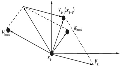
ED-PSO model updating algorithm optimization principle is the same as particle swarm algorithm, first assume that there is a swarm of particles in the space, to describe the characteristics of the particles in terms of position, velocity and adaptation value, the particles in the solution space through the individual extreme value and swarm extreme value to continuously update their own position velocity information, to derive a new adaptation value, and compare with the swarm extreme value, and finally find the assumption that in a D-dimensional search space, there are swarm particles where the -th particle can be represented as an i-dimensional vector: , the velocity of the -th particle can also be expressed as an i-dimensional vector: , the optimal position searched by the -th particle so far is called the individual extreme value: , the optimal position searched so far by the whole particle swarm is the global extreme value: , and after finding these two optimal values, the particle swarm is updated by Eqs. (5) and (6) as follows:
where denotes the inertia weight (generally taken as 0.8-1.2), 1,2,…,, 1, 2…,, refers to the number of current iterations calculated, refers to the velocity of the current particle, refers to the position of the current particle, , are acceleration factors, and , are distributed as random numbers in [0, 1]. In order to prevent the particles from searching blindly in the solution space, the numerical intervals , are generally set for the velocity and position of the particles, and the schematic diagram of the algorithm operation is shown in Fig. 1.
Fig. 1The schematic diagram of Particle Swarm Optimization
However, the natural frequency and deflection often need to be calculated, which means that if the natural frequency and deflection are directly used as the variables of the objective function, the range of the function variables cannot be directly determined, and it is not possible to randomly select a certain number of particles and iterative optimization within a certain range. However, the natural frequency and deflection are usually related to the material parameters of the structure, and the material parameters of the structure can be determined in a general range, so the ED-PSO model updating algorithm usually takes the material parameters of the structure as the object of the particle iterative optimization, and the ED-PSO model updating algorithm is implemented in the following steps:
(1) Select the studied structural material parameters and determine their ranges;
(2) Set the number of particle swarms, maximum number of iterations, inertia weights, learning factors, maximum and minimum particle positions, maximum and minimum values of motion velocity, and objective function tolerances for the ED-PSO model updating algorithm;
(3) Generate random particle swarms within the parameter setting range;
(4) Import the generated parameters into ANSYS for relevant calculations, obtain the natural frequency and deflection under each group of particles, and bring them into the objective function for comparison to obtain the local optimal particle;
(5) Enter into the iterative optimization process, as in the particle swarm algorithm, the particles are moved within the parameter setting range, and the real particles are continuously updated;
(6) Import the iterative optimization example into ANSYS for calculation, and get the corresponding natural frequency and deflection, and bring it into the objective function for calculation, and get the global optimal particle;
(7) Output the values of natural frequency and deflection at this point as the result of the model updating calculation.
3. Verification of the ED-PSO algorithm
3.1. Model updating of a reinforced concrete beam
In order to verify the superiority of the proposed ED-PSO model updating algorithm, this section takes a simply supported beam as the research object and performs the finite element model updating calculation by two methods respectively, and judges the advantages and disadvantages of the two methods by comparing the errors of the derived deflections and natural frequencies with the actual model.
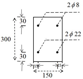
The dimensions of the simply supported beam are 3 m long, 0.15 m wide and 0.3 m high with four reinforcement bars, and the cross-sectional dimensions of the reinforced concrete beam are shown in Fig. 2.
Fig. 2Sectional dimension picture of reinforced concrete beam
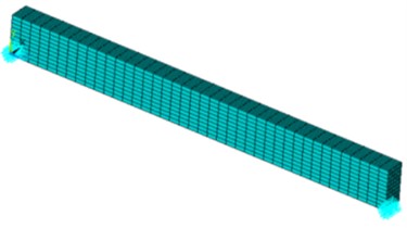
The modeling software is ANSYS APDL2021R1, which has strong finite element calculation capability and is very accurate in solving structural modal parameters and load problems. The concrete material is simulated by solid65 element, and the elastic modulus of concrete is set as 3.25×10⁴ MPa and the density is 2500 kg/m3; the reinforcement is simulated by Link180 element, and the elastic modulus of reinforcement is 2×10⁵ MPa and the density is 7850 kg/m3. The grid is divided as follows: 40 sections in the length direction of the reinforced concrete beam, 10 sections in the height and width direction, the grid shape is hexahedral cells, a total of 4000 cells, and the grid is divided by mapping, so that the grid is neatly arranged, and the constraint adopts simple support constraint, considering that the structure is a three-dimensional structure, so one end is displacement constrained in , , and directions, and the other end is displacement constrained in x and y directions with no moment constraint. The initial finite element model of the reinforced concrete beam is shown in Fig. 3.
Fig. 3Initial finite element model of reinforced concrete beam
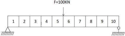
For the purpose of finite element model updating work, the reinforced concrete beam is cut into ten equal parts, each part being numbered 1-10. Apply a force of 100 KN in the middle of the reinforced concrete beam, as shown in Fig. 4.
Fig. 4Schematic diagram of reinforced concrete beam
The elastic modulus of concrete of parts No. 2, 4 and 7 is reduced by 20 % as the actual model of the reinforced concrete beam. The middle deflection of beam bottom and the first third-order natural frequencies of beam vibration under free state at the beam length ( direction) of 0.3 m, 0.6 m, 0.9 m, 1.2 m and 1.5 m under the load of 100 KN are taken as the reference data for the updating accuracy of the finite element model. According to the sectional structure of reinforced concrete beam and the calculation formula of the modal parameters of simply supported beam, it can be seen that the physical parameters that have a great influence on the modal parameters of beam structure are mainly the elastic modulus of concrete, concrete density, elastic modulus of reinforcement, section area, etc. The actual structure has equal cross-section and almost no change in cross-section, however, due to factors such as uneven mixing of concrete and impurities in reinforcement, the elastic modulus of concrete, concrete density and elastic modulus of reinforcement vary greatly, so the above three variables are selected here as the variables to be updated. Since concrete is the main material of the simply supported beam structure, the elastic modulus of concrete and density are set as local variables, according to the numbering in Fig. 3.7, the elastic modulus of concrete is set as ,concrete density is set as , and the elastic modulus of reinforcement is a global variable set to . In this way, there are 21 variables to be updated, and all parameters take values between 0.8 times and 1.2 times the design value of the parameters.
The finite element model updating numerical calculation of reinforced concrete beam is realized by ED-PSO model updating algorithm, setting the swarm size as 50, the maximum number of iterations as 200, each particle corresponds to 21 updating variables, the inertia weight w is set as 0.729, the learning factor 2, the particle position interval is the interval where the parameters take values,and the maximum and minimum value of velocity is ±0.4 times of the parameter design value.The errors of the updated frequencies and deflections with the actual model are obtained as a reference.
First, determine the value interval of the elastic modulus of concrete (), density of concrete () and elastic modulus of reinforcement (), as shown in Table 1.
Table 1Value range of parameter variable
Physical parameters | (MPa) | (kg/m3) | (MPa) |
Range of values | [2.6*104, 3.9*104] | [2000, 3000] | [1.6*105, 2.4*105] |
Since the first three orders of natural frequencies and five measured points of deflection are used as a reference for the updating results, Eq. (4) is rewritten as Eq. (7):
Because each swarm represents a 21-dimensional vector, in order to visualize the initial value of each variable in the vector, here the concrete elastic modulus, concrete density, and steel elastic modulus are combined, i.e., combined into three-dimensional coordinate points , ,…, , and the resulting random particle coordinate points are shown in Fig. 5.
By solving the particle swarm local optimum, the individual local optimum particle is obtained, at which time 2.27×10¹¹ Pa, and similarly, the individual local optimum particle is expressed in two-dimensional coordinates , ,…, , the individual local optimum particles are shown in Fig. 6, individual optimal particle values are shown in Table 2.
Fig. 5Initial particle distribution
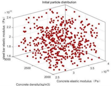
Fig. 6Individual optimal particle distribution
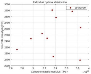
Table 2Local optimization of random particles
(MPa) | (kg/m3) | (MPa) | |
1 | 3.16×10⁴ | 2522 | 2.27×10⁵ |
2 | 3.84×10⁴ | 2090 | |
3 | 3.34×10⁴ | 2904 | |
4 | 3.70×10⁴ | 2884 | |
5 | 2.96×10⁴ | 2439 | |
6 | 3.41×10⁴ | 2782 | |
7 | 3.36×10⁴ | 2148 | |
8 | 3.85×10⁴ | 2620 | |
9 | 2.71×10⁴ | 2261 | |
10 | 3.25×10⁴ | 2446 |
Import the above data into ANSYS as a text file, solve the structure’s natural frequency and deflection, and compare with the actual structure. The graphs of the first three orders of modal analysis of the reinforced concrete beam under load are shown in Fig. 7.
Fig. 7Diagram of first third order vibration and load deformation of beam
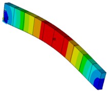
a) First order vibration
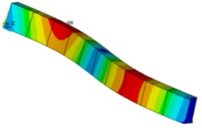
b) Second order vibration
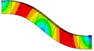
c) Third order vibration
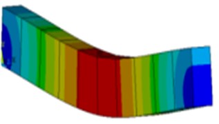
d) Load deformation
Then set the parameters of the actual structure, calculate the corresponding deflection and natural frequency in the case of the actual structure, and finally calculate the deflection and natural frequency of the structure to be updated in the individual optimal case as the result before the model updating, and calculate the error of the deflection and natural frequency of the model to be updated with the actual structure by Eq. (8) and Eq. (9):
The final relevant calculation results are shown in Table 3.
Table 3Data before beam updating
Description | Initial value | Actual value | Error (%) |
Deflection at 0.3 m (mm) | 6.19 | 6.70 | 7.61 |
Deflection at 0.3 m (mm) | 13.09 | 14.32 | 8.59 |
Deflection at 0.3 m (mm) | 19.47 | 21.28 | 8.51 |
Deflection at 0.3 m (mm) | 24.25 | 26.43 | 8.25 |
Deflection at 0.3 m (mm) | 26.24 | 28.38 | 7.54 |
First order frequency (Hz) | 78.04 | 76.67 | 1.79 |
Second order frequency (Hz) | 129.38 | 122.94 | 5.24 |
Third order frequency (Hz) | 159.01 | 161.34 | 1.44 |
The global optimal particle is then solved, at which point 1.85×10¹¹ Pa, and the two-dimensional coordinates of the variables taken are shown in Fig. 8. The global optimal particle results are shown in Table 4.
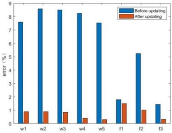
Similarly, save the calculated global optimal particles to a text file, and then import the data into ANSYS for the solution of deflection and natural frequency, and then carry out the error calculation of the deflection under the actual structure, the results of which are shown in Table 5. The updated error is obtained and compared with the pre-updating error, as shown in Fig. 9.
It is easy to see from the obtained data that the ED-PSO model updating algorithm has a high updating accuracy for the finite element model updating method.
Table 4Global optimization of random particles
(MPa) | (kg/m3) | (MPa) | |
1 | 3.10×10⁴ | 2549 | 1.85×10⁵ |
2 | 2.75×10⁴ | 2042 | |
3 | 3.30×10⁴ | 2334 | |
4 | 3.25×10⁴ | 2385 | |
5 | 2.80×10⁴ | 2458 | |
6 | 2.95×10⁴ | 2120 | |
7 | 3.47×10⁴ | 2619 | |
8 | 3.21×10⁴ | 2245 | |
9 | 3.13×10⁴ | 2331 | |
10 | 3.23×10⁴ | 2355 |
Table 5Data after beam updating
Description | Initial value | Actual value | Error (%) |
Deflection at 0.3 m (mm) | 6.64 | 6.70 | 0.89 |
Deflection at 0.3 m (mm) | 14.19 | 14.32 | 0.90 |
Deflection at 0.3 m (mm) | 21.09 | 21.28 | 0.86 |
Deflection at 0.3 m (mm) | 26.32 | 26.43 | 0.40 |
Deflection at 0.3 m (mm) | 28.46 | 28.38 | 0.31 |
First order frequency (Hz) | 77.82 | 76.67 | 1.51 |
Second order frequency (Hz) | 124.19 | 122.94 | 1.02 |
Third order frequency (Hz) | 161.85 | 161.34 | 0.32 |
Fig. 8Global optimal particle distribution
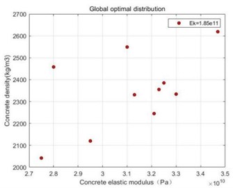
Fig. 9Error comparison before and after updating
3.2. Comparison with CSD-PSO
In order to verify the advantages of the proposed method, simply supported beams in the previous section are used as the research object in this section, and performs the model updating calculation by the previous study - the combination of static and dynamic methods and particle swarm algorithm (CSD-PSO), and compares the results with the proposed method, and the results show that the proposed method has higher accuracy.
Particle swarm algorithm-based finite element model updating techniques combined with a variety of objective functions, model updating accuracy reference data are mainly natural frequency, deflection, etc.[34], static and dynamic methods are commonly used to measure the above data. The data measured by the static method are more accurate and easier to measure, but the measured data cannot reflect the dynamic changes of the structure. The data measured by dynamic method is less accurate and the testing process is tedious, but it can reflect the dynamic changes of the structure. In order to combine the advantages of the two, the combination of static and dynamic methods of finite element model updating was produced and widely used in the study of finite element model updating. However, while the combination of static and dynamic methods combines the advantages of both, it also amplifies the disadvantages of both, and the combination of static and dynamic methods requires more objective functions and is more complicated to calculate. The commonly used objective function of the combination of static and dynamic methods is shown in Eq. (10) [35]:
where and are the dynamic and static objective functions of the structure, respectively. The objective function of the combination of static and dynamic methods is shown in 3.4, where and are the dynamic and static objective functions of the reinforced concrete beam, respectively, as shown in Eqs. (11 and 12):
where and denote the first three orders of natural frequencies calculated by the actual structure and the first three orders of natural frequencies calculated by the model to be updated, respectively. , denote the middle deflection of the bottom of the beam at 0.3 m, 0.6 m, 0.9 m, 1.2 m and 1.5 m in the direction of the length of the extended beam under the load action of the actual structure and the structure to be updated, respectively.
As in the previous subsection, the range of values of concrete modulus of elasticity, concrete density, and steel modulus of elasticity is still the same as the range of values in Table 1.Similarly,50 sets of particle vectors are randomly generated, and each variable will be expressed in three-dimensional coordinate points , ,…,, the resulting random particle coordinate points are shown in Fig. 10.
Fig. 10Initial particle distribution
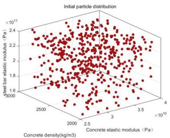
Fig. 11Individual optimal particle distribution
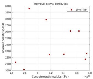
Similarly, the optimal value among the 50 particle vectors is found by performing a local optimization search calculation, at which time 2.11×10¹¹ Pa, and the individual optimal particles are expressed in two-dimensional coordinates , ,…, , the results are shown in Fig. 11. The specific values of each parameter variable are shown in Table 6. Save the calculated individual optimal particles to a text file, and then import the data into ANSYS for the solution of the deflection and natural frequency, and the final calculation results are shown in Table 7.
Table 6Local optimization of random particles
(MPa) | (kg/m3) | (MPa) | |
1 | 3.18×10⁴ | 2246 | 2.11×10⁵ |
2 | 3.73×10⁴ | 2173 | |
3 | 3.75×10⁴ | 2260 | |
4 | 2.87×10⁴ | 2957 | |
5 | 3.63×10⁴ | 2609 | |
6 | 3.5×10⁴ | 2609 | |
7 | 3.4×10⁴ | 2250 | |
8 | 3.13×10⁴ | 2785 | |
9 | 2.79×10⁴ | 2011 | |
10 | 2.66×10⁴ | 2123 |
Table 7Data before beam updating
Description | Initial value | Actual value | Error (%) |
Deflection at 0.3 m (mm) | 6.39 | 6.70 | 4.58 |
Deflection at 0.3 m (mm) | 13.45 | 14.32 | 6.06 |
Deflection at 0.3 m (mm) | 19.95 | 21.28 | 6.23 |
Deflection at 0.3 m (mm) | 24.75 | 26.43 | 6.36 |
Deflection at 0.3 m (mm) | 26.54 | 28.38 | 6.46 |
First order frequency (Hz) | 78.38 | 76.67 | 2.23 |
Second order frequency (Hz) | 127.66 | 122.94 | 3.84 |
Third order frequency (Hz) | 169.07 | 161.34 | 4.79 |
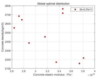
The global optimal particle distribution is obtained by the global iterative optimization search of the particle swarm algorithm, at which time 2.37×10¹¹ Pa, similarly, the individual optimal particles are represented by two-dimensional coordinates , ,…, , the global optimal particle distribution is shown in Fig. 12. The specific values of the global optimal particles are shown in Table 8.
Fig. 12Global optimal particle distribution
Save the calculated global optimal particles to a text file, and then import the data into ANSYS for the solution of deflection and natural frequency, and the error is calculated with the deflection under the actual structure, and the calculated results are shown in Table 9. The error after updating is compared with the error before updating, as shown in Fig. 13.
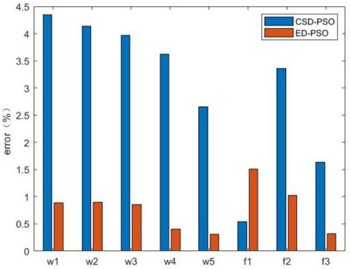
Compare the error of the updated data of the model updating method ED-PSO model updating algorithm and CSD-PSO model updating algorithm, and the result is shown in Fig. 14.
As can be seen from Fig. 14, ED-PSO model updating algorithm is obviously superior to CSD-PSO model updating algorithm.
Table 8Global optimization of random particles
(Mpa) | (kg/m3) | (MPa) | |
1 | 3.35×10⁴ | 2171 | 2.37×10⁵ |
2 | 2.77×10⁴ | 2643 | |
3 | 2.89×10⁴ | 2385 | |
4 | 2.72×10⁴ | 2684 | |
5 | 3.16×10⁴ | 2453 | |
6 | 2.64×10⁴ | 2553 | |
7 | 3.46×10⁴ | 2717 | |
8 | 3.74×10⁴ | 2156 | |
9 | 3.81×10⁴ | 2217 | |
10 | 3.46×10⁴ | 2765 |
Table 9Data after beam updating
Description | Initial value | Actual value | Error (%) |
Deflection at 0.3 m (mm) | 6.41 | 6.70 | 4.35 |
Deflection at 0.3 m (mm) | 13.73 | 14.32 | 4.14 |
Deflection at 0.3 m (mm) | 20.43 | 21.28 | 3.97 |
Deflection at 0.3 m (mm) | 25.47 | 26.43 | 3.62 |
Deflection at 0.3 m (mm) | 27.62 | 28.38 | 2.65 |
First order frequency (Hz) | 77.09 | 76.67 | 0.54 |
Second order frequency (Hz) | 127.08 | 122.94 | 3.36 |
Third order frequency (Hz) | 158.69 | 161.34 | 1.64 |
Fig. 13Error comparison before and after updating
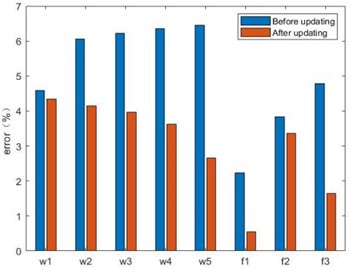
Fig. 14Error comparison of two methods
4. Conclusions
At present, there are many optimization algorithms used to solve the optimization problem of finite element model updating. The finite element model updating based on particle swarm optimization algorithm is popular at present, and there are relatively many objective functions combined with it. This paper firstly propose the ED-PSO model updating algorithm, and a simply supported beam is taken as the research object, and the numerical calculation of finite element model updating is carried out. By comparing the calculation results with previous research on CSD-PSO model updating algorithm. The results show that the ED-PSO model updating algorithm has obvious advantages.
References
-
H. Liu, G. Song, Y. Jiao, P. Zhang, and X. Wang, “Damage identification of bridge based on modal flexibility and neural network improved by particle swarm optimization,” Mathematical Problems in Engineering, Vol. 2014, pp. 1–8, 2014, https://doi.org/10.1155/2014/640925
-
J.-T. Kim, J.-H. Park, and B.-J. Lee, “Vibration-based damage monitoring in model plate-girder bridges under uncertain temperature conditions,” Engineering Structures, Vol. 29, No. 7, pp. 1354–1365, Jul. 2007, https://doi.org/10.1016/j.engstruct.2006.07.024
-
M. Döhler, F. Hille, L. Mevel, and W. Rücker, “Structural health monitoring with statistical methods during progressive damage test of S101 Bridge,” Engineering Structures, Vol. 69, No. 9, pp. 183–193, Jun. 2014, https://doi.org/10.1016/j.engstruct.2014.03.010
-
M. Sanayei, A. Khaloo, M. Gul, and F. Necati Catbas, “Automated finite element model updating of a scale bridge model using measured static and modal test data,” Engineering Structures, Vol. 102, No. 1, pp. 66–79, Nov. 2015, https://doi.org/10.1016/j.engstruct.2015.07.029
-
Andrea Mordini, Konstantin Savov, and Helmut Wenzel, “The finite element model updating: a powerful tool for structural health monitoring,” Structural Engineering International, Vol. 17, No. 4, p. 352, 1992.
-
N. F. Alkayem, M. Cao, Y. Zhang, M. Bayat, and Z. Su, “Structural damage detection using finite element model updating with evolutionary algorithms: a survey,” Neural Computing and Applications, Vol. 30, No. 2, pp. 389–411, Jul. 2018, https://doi.org/10.1007/s00521-017-3284-1
-
E. M. Hernandez and D. Bernal, “Iterative finite element model updating in the time domain,” Mechanical Systems and Signal Processing, Vol. 34, No. 1-2, pp. 39–46, Jan. 2013, https://doi.org/10.1016/j.ymssp.2012.08.007
-
Y. Q. Li and Y. L. Du, “Dynamic finite element model updating of stay-cable based on the most sensitive design variable,” (in Chinese), Journal of Vibration and Shock, Vol. 28, No. 3, pp. 141–143, 2009.
-
B. P. Wang and S. P. Caldwell, “An improved approximate method for computing eigenvector derivatives,” in Finite Elements in Analysis and Design, Vol. 14, No. 4, pp. 381–392, Nov. 1993, https://doi.org/10.1016/0168-874x(93)90035-o
-
G. Canbaloğlu and H. N. Özgüven, “Model updating of nonlinear structures from measured FRFs,” Mechanical Systems and Signal Processing, Vol. 80, pp. 282–301, Dec. 2016, https://doi.org/10.1016/j.ymssp.2016.05.001
-
B. Naderi, M. Zandieh, A. Khaleghi Ghoshe Balagh, and V. Roshanaei, “An improved simulated annealing for hybrid flowshops with sequence-dependent setup and transportation times to minimize total completion time and total tardiness,” Expert Systems with Applications, Vol. 36, No. 6, pp. 9625–9633, Aug. 2009, https://doi.org/10.1016/j.eswa.2008.09.063
-
M. R. Banan, M. R. Banan, and K. D. Hjelmstad, “Parameter estimation of structures from static response. i. computational aspects,” Journal of Structural Engineering, Vol. 120, No. 11, pp. 3243–3258, Nov. 1994, https://doi.org/10.1061/(asce)0733-9445(1994)120:11(3243)
-
J. D. Collins, G. C. Hart, T. K. Hasselman, and B. Kennedy, “Statistical identification of structures,” AIAA Journal, Vol. 12, No. 2, pp. 185–190, Feb. 1974, https://doi.org/10.2514/3.49190
-
J. Brownjohn, P. Moyo, P. Omenzetter, and Yong Lu, “Assessment of highway bridge upgrading by dynamic testing and finite element model updating,” Journal of Bridge Engineering, Vol. 8, No. 6, pp. 162–172, 2003.
-
H. Ebrahimian, R. Astroza, J. P. Conte, and R. A. de Callafon, “Nonlinear finite element model updating for damage identification of civil structures using batch Bayesian estimation,” Mechanical Systems and Signal Processing, Vol. 84, pp. 194–222, Feb. 2017, https://doi.org/10.1016/j.ymssp.2016.02.002
-
J. E. Mottershead, M. Link, and M. I. Friswell, “The sensitivity method in finite element model updating: A tutorial,” Mechanical Systems and Signal Processing, Vol. 25, No. 7, pp. 2275–2296, Oct. 2011, https://doi.org/10.1016/j.ymssp.2010.10.012
-
E. Görl and M. Link, “Damage identification using changes of eigenfrequencies and mode shapes,” Mechanical Systems and Signal Processing, Vol. 17, No. 1, pp. 103–110, Jan. 2003, https://doi.org/10.1006/mssp.2002.1545
-
Sheng-En Fang, Ricardo Perera, and Guido de Roec, “Damage identification of a reinforced concrete frame by finite element model updating using damage parameterization,” Journal of Sound and Vibration, Vol. 313, pp. 544–559, 2008, https://doi.org/10.1016/jjsv.2007.11.057
-
Moaveni B., Stavridis A., and Lombaert G., “Finite-element model updating for assessment of progressive damage in a 3-story infilled RC frame,” Journal of Structural Engineering, Vol. 139, No. 10, p. 1665, 1674.
-
G. Pinte, B. Depraetere, W. Symens, J. Swevers, and P. Sas, “Iterative learning control for the filling of wet clutches,” Mechanical Systems and Signal Processing, Vol. 24, No. 7, pp. 1924–1937, 2010, https://doi.org/10.1016/jymssp.2010.05.016
-
S. Weng, Y. Xia, Y.-L. Xu, and H.-P. Zhu, “Substructure based approach to finite element model updating,” Computers and Structures, Vol. 89, No. 9-10, pp. 772–782, May 2011, https://doi.org/10.1016/j.compstruc.2011.02.004
-
X. Qian, M. Cao, Z. Su, and J. Chen, “A hybrid particle swarm optimization (PSO)-simplex algorithm for damage identification of delaminated beams,” Mathematical Problems in Engineering, Vol. 2012, pp. 1–11, 2012, https://doi.org/10.1155/2012/607418
-
Y. Zhang, D. Gallipoli, and C. E. Augarde, “Simulation-based calibration of geotechnical parameters using parallel hybrid moving boundary particle swarm optimization,” Computers and Geotechnics, Vol. 36, No. 4, pp. 604–615, May 2009, https://doi.org/10.1016/j.compgeo.2008.09.005
-
Y. Lin, W. Chang, and J. Hsieh, “A particle swarm optimization approach to nonlinear rational filter modeling,” Expert Systems with Applications, Vol. 34, No. 2, pp. 1194–1199, Feb. 2008, https://doi.org/10.1016/j.eswa.2006.12.004
-
R. Kathiravan and R. Ganguli, “Strength design of composite beam using gradient and particle swarm optimization,” Composite Structures, Vol. 81, No. 4, pp. 471–479, Dec. 2007, https://doi.org/10.1016/j.compstruct.2006.09.007
-
T. Vo-Duy, V. Ho-Huu, H. Dang-Trung, and T. Nguyen-Thoi, “A two-step approach for damage detection in laminated composite structures using modal strain energy method and an improved differential evolution algorithm,” Composite Structures, Vol. 147, No. 1, pp. 42–53, Jul. 2016, https://doi.org/10.1016/j.compstruct.2016.03.027
-
L. Liu, W. Liu, and D. A. Cartes, “Particle swarm optimization-based parameter identification applied to permanent magnet synchronous motors,” Engineering Applications of Artificial Intelligence, Vol. 21, No. 7, pp. 1092–1100, Oct. 2008, https://doi.org/10.1016/j.engappai.2007.10.002
-
R. E. Perez and K. Behdinan, “Particle swarm approach for structural design optimization,” Computers and Structures, Vol. 85, No. 19-20, pp. 1579–1588, Oct. 2007, https://doi.org/10.1016/j.compstruc.2006.10.013
-
R. Hassan, B. Cohanim, O. de Weck, and G. Venter, “A comparison of particle swarm optimization and the genetic algorithm,” in 46th AIAA/ASME/ASCE/AHS/ASC Structures, Structural Dynamics and Materials Conference, pp. 18–21, Apr. 2005, https://doi.org/10.2514/6.2005-1897
-
Y. Otsuki, D. Li, X. Dong, and Y. Wang, “SMU – an open-source MATLAB package for structural model updating,” Bridge Maintenance, Safety, Management, Life-Cycle Sustainability and Innovations, pp. 1621–1628, Apr. 2021, https://doi.org/10.1201/9780429279119-222
-
E. T. Lee and H. C. Eun, “Update of updated stiffness and ass matrices based on measured dynamic modal data,” Applied Mathematical Modelling, Vol. 33, No. 5, pp. 2274–2281, 2009.
-
D. Li, X. Dong, and Y. Wang, “Model updating using sum of squares (SOS) optimization to minimize modal dynamic residuals,” Structural Control and Health Monitoring, Vol. 25, No. 12, 2018.
-
W.-Q. Sun and W. Cheng, “Finite element model updating of honeycomb sandwich plates using a response surface model and global optimization technique,” Structural and Multidisciplinary Optimization, Vol. 55, No. 1, pp. 121–139, Jan. 2017, https://doi.org/10.1007/s00158-016-1479-1
-
Hua Z., “Dynamic and static-based finite element model updating of bridge structures,” Fuzhou University, 2006.
-
M. M. Saada, M. H. Arafa, and A. O. Nassef, “Finite element model updating approach to damage identification in beams using particle swarm optimization,” Engineering Optimization, Vol. 45, No. 6, pp. 677–696, Jun. 2013, https://doi.org/10.1080/0305215x.2012.704026
About this article

This work was supported by the Jiangsu International Joint Research and Development Program [BZ2022010]; Anhui international joint research center of data diagnosis and smart maintenance on bridge structures (Grant No. 2021AHGHYB06); and the Nanjing International Joint Research and Development Program [202112003].
The datasets generated during and/or analyzed during the current study are available from the corresponding author on reasonable request.
Can Wang was responsible for formal analysis, methodology, software, and writing-original draft preparation. Dayang Li was responsible for conceptualization, funding acquisition, visualization, and writing-review and editing. Panida Kaewniam was responsible for investigation, supervision, and validation. Jie Wang was responsible for investigation, funding acquisition, and resources. Tareq Al-hababi was responsible for investigation, funding acquisition, and supervision.
The authors declare that they have no conflict of interest.
