Abstract
This paper presents two eigenfrequency-based damage diagnosis methods in a cantilever beam. The analytical relationship has been established between the eigenfrequency and damage parameters, including relative damage location and severity. On the premise that pre-damaged eigenfrequencies are known, a diagnosis algorithm without requirement of material properties is proposed based on change ratios of the first three eigenfrequencies. If pre-damaged eigenfrequencies are unfeasible to be acquired, a three-contour method based on only post-damaged eigenfrequencies is introduced to estimate damage parameters. The uniqueness of solution is discussed. Both the numerical simulation by the finite element method and the experiment on real beams are conducted and result in a good agreement between actual damage parameters and calculated values by using the proposed methods.
1. Introduction
Structural damages, caused by material aging, impact, fatigue, chemical attack and other unexpected mechanical loadings, may cause the performance degradation or even lead to the catastrophic failure in a structure. In the past few decades, a significant amount of analytical, numerical and experimental investigations has been carried out to detect damages at earliest possible stages through measuring and analyzing changes of modal properties on a damaged structure [1-4], based on the principle that a localized damage reduces the stiffness and increase the damping in the structure thus further decreases the eigenfrequency and alters the mode shape. Compared with nondestructive examination methods (NDE), such as X-ray imaging, ultrasonic scans and eddy current testing, et al, the modal-parameter-based damage diagnosis technique is more sufficient to cater for the needs of long range, quick global inspection and in service inspection of structures.
Eigenfrequency is one of the most popular modal properties used in damage identification due to its attractive characteristic of being relatively easy to be measured in a high precision. However, the frequency-based method can be only applied to typical structures and damages which can be theoretically modeled through mathematical approximations. Beam is one of the simplest and most commonly used structures, and a variety of complex structures are comprised of beams, hence the fundamental theory of the frequency-based damage identification technique is established on the beam-type structure, especially on the slender Eular-Bernoulli beam. Usually, an open transverse edge crack is considered as the typical localized damage. The crack is theoretically equivalent to a massless linear torsional spring, and the beam is treated as two segmental beams connected by the spring. The earliest spring model was the axial spring proposed by Adams et al. [5], however, the theory to quantitatively analyze the equivalent spring stiffness did not be constructed. Then, a rotational elastic spring model was developed by Papadopoulos et al. [6], the equivalent spring stiffness of which was given as a function of the damage severity. Based on this model, Rizos et al. [7] arose an 8×8 determinantal equation relating the eigenfrequency, damage parameters (damage location and damage severity) and material properties (Young's modulus and density) for a cantilever beam. Other researchers then developed similar equations for beams with different boundary conditions. Ostachowicz et al. [8] deduced analytical expressions of equivalent spring stiffnesses of two different damages, open double-side crack and open single-side crack. Their conclusions indicated that the equivalent spring stiffness is a function of only the damage severity, with no relationship with the damage location. They also constructed the mathematical relationship between the eigenfrequency, damage parameters and material properties in the form of a 12×12 determinantal equation for a cantilever beam with the assumption of two cracks. Liang et al. [9] proposed an approach based on any three eigenfrequencies to determine damage parameters in a cantilever beam or a simply supported beam. The method treats the crack as a rotational spring, plots the relationship curve between the equivalent stiffness and the damage location for each eigenfrequency, and determines the stiffness and the damage location in the intersection of three curves. The damage severity is then calculated from the relationship formula of the equivalent stiffness and the damage severity. This approach was then extended to stepped beams by Nandawana et al. [10] and geometrically segmented beams by Chaudhari et al. [11]. Owolabi et al. [12] presented a similar three-contour method based on any three eigenfrequencies. In this method, the three-dimensional curved surface of each eigenfrequency in terms of the damage location and severity is obtained through the determinantal equation, and then the contour on the surface corresponding to the measured eigenfrequency value is projected onto the location-severity coordinate plane. The intersection of three contours points out the damage location and severity.
These above mentioned methods detect the damage using post-damaged eigenfrequencies only, with no requirement of corresponding pre-damaged eigenfrequencies. However, in these methods, it is necessary to know material properties which are normally inconvenient to be measured in practice and solve a complicated determinantal equation. Plenty of effort has been devoted to frequency-change-based methods to overcome this problem. Cawlay et al. [13] proved that the ratio of eigenfrequency changes for two modes is only related with the damage location but no damage severity. Hearn et al. [14] also demonstrated that for a structure with a single damage, the variation ratio of squared eigenfrequency is a function of the damage location only. Narkis et al. [15] deduced a theoretical formula to describe relationship between the damage location and the ratio of eigenfrequency variations for a simply supported beam in the transverse vibration and the longitudinal vibration, and for a free-free beam in the longitudinal vibration. On the assumption that the crack is very small and leads to no volume change, Gudmundson [16] concluded a linear relationship between the fractional change of eigenfrequency and that of modal strain energy via the first order perturbation method. Based on Gudmundson's theory, Kim et al. [17, 18] studied the relationship between damage parameters and the variation ratio of eigenfrequency, and proposed an indicator for the single damage. The indicator is defined as the difference between the variation ratio of modal strain energy and that of eigenfrequency, and it reaches maximum at the damage position. Rubio [19] gave a relationship formula between the square ratio of the post-damaged eigenfrequency to the pre-damaged eigenfrequency and damage parameters for a simply-supported beam, and employed an optimization technique by minimizing a least square criterion to determine the damage location and severity. Sayyad et al. proposed an eigenfrequency-change-based damage diagnosis algorithm for beam structures with simply supported [20] and cantilever [21, 22] boundary conditions. They got a right algorithm for the simply supported beam, but mistook the mode shape of the simply supported beam for that of the cantilever beam and thus drew an erroneous conclusion for the cantilever beam. In frequency-change based methods, no material property is demanded, but an accurate knowledge of pre-damaged eigenfrequencies is indispensable. Unfortunately, it is unfeasible to meet the healthy structure in many real applications. Normally, the finite element method (FEM) is employed to model the structure, but as we know, the numerical simulation asks for material properties.
In this paper, two methods are proposed to diagnose the damage in a cantilever beam, for situations with and without eigenfrequencies of the indefective beam. The relationship formula between damage parameters and the variation ratio of eigenfrequencies is established, with no material property. If eigenfrequencies of the intact beam can be acquired, an eigenfrequency-change-based method is presented. Algebraic equations based on the first three eigenfrequencies, related to the damage location only, are deduced from the relationship formula. The damage location is indicated by solving the equations, and then fed to the relationship formula to determine the damage severity. Analysis of the uniqueness of solution to the algebraic equations is carried out, which is always lacking in other eigenfrequency-based approaches. If frequencies of the intact beam are absent, a post-damaged-eigenfrequency-based three-contour method is introduced to determine the damage location and severity. This method gains an advantage of being material-property-free over other three-curve methods. Numerical simulations and experiments are conducted to verify the proposed methods. The results show that an accurate evaluation of both the damage location and the damage severity can be achieved with an error which is acceptable in practical applications by using the proposed methods.
2. Theoretical analysis for damage identification
2.1. Eigenfrequency-change-based method
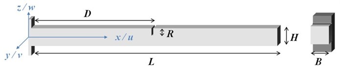
A typical Euler-Bernoulli cantilever beam damaged by a small discrete single-side crack is considered, and a Cartesian coordinate system -- is established, as shown in Fig. 1. The length, height and width of the beam are , and , respectively. The crack of a depth , which is supposed to remain open during vibrations, is at the position of distance to the clamping end. Normally, the relative position is used to represent the dimensionless crack location and the relative depth is used to represent the dimensionless crack severity. Young’s modulus and mass density are represented by and , respectively. For the convenience of deduction and calculation, another Cartesian coordinate system -- is established as well, in which , , , hence the length, height and width of the beam in the new coordinate system are 1, , , respectively.
Fig. 1An Euler-Bernoulli cantilever beam model with a single edge crack
Presuming the crack is small enough to cause no volume change, the following relationship between the fractional change of eigenfrequency and that of modal strain energy is proposed by Gudmundson [16]:
where and are the angular eigenfrequencies before and after the crack occurrence, and subscript demotes the thmode, respectively. Considering that the eigenfrequency difference is very small, the sum of and is feasible to be regarded as a double value of , hence the following relationship formula can be acquired:
where is the eigenfrequency change. In order to satisfy the assumption, usually, the relative depth is restricted in the region (0, 0.5). The restriction is reasonable for damage detection at earliest possible stages.
The th modal strain energy of an undisturbed Euler-Bernoulli beam in the -- coordinates is given as follows [17]:
where is the th mode shape.
For an Euler-Bernoulli beam structure with an edge crack under bending, the stress intensity factor is [23]:
where is a geometrical factor expressed as Eq. (5) and is the stress level given by Eq. (6) with regard to a plane state of stress:
Hence, the strain energy density function can be obtained as follows:
The decrease of modal strain energy is:
where is the area of the crack damage. Since :
Since , it’s convenient to convert Eq. (9) to the following form:
Substituting Eq. (3) and (10) into Eq. (2), the following equation can be got:
where and .
The mode shape of an Euler-Bernoulli cantilever beam is given as:
where:
Therefore:
For the first mode ( 1), 1.875, thus 12.3623. Similarly, 485.52, 3806.2. Since is a constant for a certain crack, it can be eliminated in division between any pair of eigenfrequency change ratios. Therefore, the following equations can be obtained:
The relative damage location can be determined by solving the equations using the Newton-Raphson method.
2.2. Analysis of uniqueness of solution
Each sub-equation in the above mentioned Eq. (14) can be solved independently, but each sub-equation has several solutions. Let , and , then the logarithmic values of , and in the -interval (0, 1) are plotted in Fig. 2.
The function is monotone increasing in the interval (0, 0.217] and monotone decreasing in the interval (0.217, 1), as shown in Fig. 2(a). The maximum value of in the interval (0.364, 1) is smaller than that in the interval (0, 0.217], thus Eq. (14a) has only one solution in the interval (0.364, 1). If the damage is located in this interval, there is only one simultaneous solution of three sub-equations. In the interval (0, 0.364], Eq. (14a) has two solutions, one of which in the interval (0, 0.217] and the other is in (0.217, 0.364].
As shown in Fig. 2(b), values of in (0, 0.167] and (0.167, 0.364] are different, considering that Eq. (14a) has only one solution in the interval (0, 0.167], thus if the damage is located in (0, 0.167], it can be determined by the simultaneous solution of Eqs. (14a) and (14b). In the interval (0.167, 0.364], Eq. (14b) also has two solution, in the intervals (0.167, 0.217] and (0.217, 0.364], respectively.
In that case, consider values of in the interval (0.167, 0.364]. As shown in Fig. 2(c), is monotone decreasing in the interval (0.167, 0.318], and the minimum of in (0.167, 0.318] is larger than that in (0.318, 0.364]. That means there exist only one simultaneous solution of the three sub-equations in (0.167, 0.318]. In (0.318, 0.364], decreases first and then increases, therefore Eq. (14c) may have two solutions. However, either of Eq. (14a) and (14b) has only one solution in this interval, thus the three sub-equations also have only one simultaneous solution.
To sum up, there exist one and only one solution for Eq. (14) in the -interval (0, 1), indicating the relative damage location .
According to Eq. (11), the variation of normalized post-damaged eigenfrequency versus relative damage location can be obtained, as shown in Fig. 3. The normalized post-damaged eigenfrequency is defined as the ratio of post-damaged to pre-damaged eigenfrequency. It’s worth noting that the exact value is determined not only the relative location but also other parameters in Eq. (11), thus the curve in Fig. 3 shows only the general variation trend versus relative location. Evidently, all the three normalized eigenfrequencies approach to 1 near the free end. The second normalized eigenfrequency approaches to 1 while is close to 0.217 and the third normalized eigenfrequency approaches to 1 while is close to 0.133 or 0.5. Being equal to 1 means that the pre-damaged and post-damaged eigenfrequencies are the same. In practical applications, when the damage is located near 1, 0.133, 0.217 or 0.5, the measured post-damaged eigenfrequency may be higher than the pre-damaged eigenfrequency because of the measurement error, thus generally speaking, a tiny plus value of ought to be chosen for calculation instead of the measured value.
Fig. 2Variation curves of gau, gbu, gcu versus relative damage location
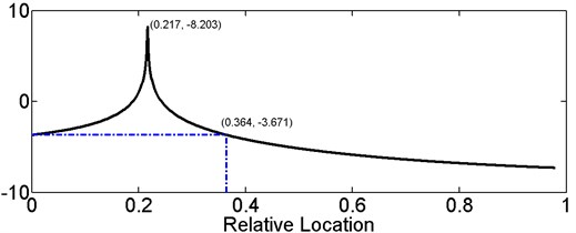
a)
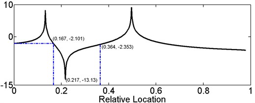
b)
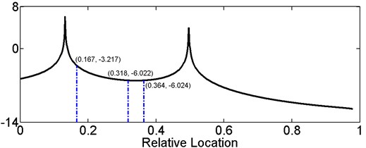
c)
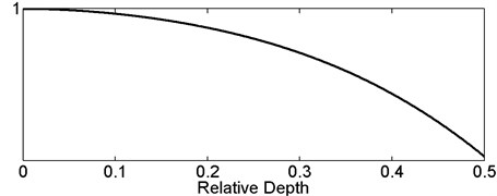
The damage severity can be computed by Eq. (11) after the acquirement of Any eigenfrequency decreases with the increase of due to the monotone increasing function in (0, 0.5), as shown in Fig. 4, thus is able to be determined via any sub-equation.
2.3. Eigenfrequency-based three-contour method
If the pre-damaged eigenfrequency is absent, transform Eq. (11) into:
hence, the post-damaged eigenfrequency is:
Fig. 3General variation trend curve of first, second and third normalized post-damaged eigenfrequency versus relative damage location
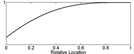
a) First
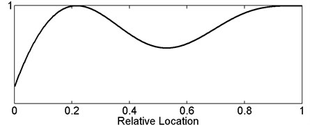
b) Second
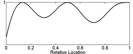
c) Third
Fig. 4General variation trend curve of normalized post-damaged eigenfrequency versus relative damage depth
As we know, the analytic eigenfrequency of an undisturbed Euler-Bernoulli beam is:
therefore, Eq. (15) is equivalent to the following:
In that case, it can be obtained:
Since Eq. (19) is deduced from Eq. (11), there is only one common solution in the -interval (0, 1) and -interval (0, 0.5) for the three sub-equations, notwithstanding that each sub-equation has infinitely many solutions. By using the three-contour method, damage parameters can be determined with the first three eigenfrequencies and dimensional sizes of the beam. Material properties are needless, which are more difficult to be measured than dimensional sizes in practice.
3. Numerical simulation
The proposed two methods, one based on the eigenfrequency change and one based on only the post-damaged eigenfrequency, were testified by both the numerical simulation and the experiment. An intact steel cantilever beam and a series of damaged beams, of length 330 mm, width 15 mm and height 12 mm, were modeled by FEM. Young’s modulus 7803 kg/m2, mass density 207 GPa and Poisson's ratio 0.3, respectively. Each damaged beam contained an open single-side notch crack, but on different beam the crack was of different depth at different position. The first three eigenfrequencies of the undamaged beam are 81.466 Hz, 507.77 Hz and 1409.6 Hz, respectively, and that of cracked beams are listed in Table 1.
Table 1First three eigenfrequencies of damaged beams simulated by FEM
0.2 | 0.3 | e=0.4 | 0.5 | 0.6 | 0.7 | 0.8 | |
0.1 | |||||||
1st eigenfrequency | 81.132 | 81.244 | 81.331 | 81.393 | 81.434 | 81.457 | 81.468 |
2nd eigenfrequency | 507.75 | 507.39 | 506.43 | 505.80 | 505.95 | 506.68 | 507.41 |
3rd eigenfrequency | 1408.0 | 1405.1 | 1407.3 | 1409.6 | 1406.6 | 1403.5 | 1405.7 |
0.2 | |||||||
1st eigenfrequency | 80.223 | 80.635 | 80.957 | 81.191 | 81.342 | 81.427 | 81.466 |
2nd eigenfrequency | 507.71 | 506.32 | 502.75 | 500.42 | 500.97 | 503.67 | 506.41 |
3rd eigenfrequency | 1403.4 | 1392.8 | 1401.0 | 1409.6 | 1398.6 | 1387.0 | 1394.7 |
0.3 | |||||||
1st eigenfrequency | 78.67 | 79.578 | 80.301 | 80.83 | 81.177 | 81.371 | 81.458 |
2nd eigenfrequency | 507.62 | 504.47 | 496.47 | 491.29 | 492.4 | 498.37 | 504.62 |
3rd eigenfrequency | 1395.6 | 1372.4 | 1390.5 | 1409.5 | 1385.3 | 1359.7 | 1375.4 |
0.4 | |||||||
1st eigenfrequency | 76.257 | 77.894 | 79.232 | 80.233 | 80.899 | 81.275 | 81.441 |
2nd eigenfrequency | 507.48 | 501.58 | 486.79 | 477.31 | 478.98 | 489.72 | 501.60 |
3rd eigenfrequency | 1383.5 | 1342.1 | 1374.8 | 1409.4 | 1365.7 | 1319.2 | 1344.0 |
In the eigenfrequency-change-based approach, the crack location was calculated using Eq. (14), and then it is put into Eq. (11) to determine the crack depth. Results are listed in Table 2. Relative errors are calculated and listed as well, which are very small and demonstrate the accuracy of the proposed method.
Table 2Damage parameters calculated by the eigenfrequency-change-based method
0.2 | 0.3 | e=0.4 | 0.5 | 0.6 | 0.7 | 0.8 | |
0.1 | |||||||
Calculated | 0.200 | 0.300 | 0.402 | 0.498 | 0.600 | 0.697 | 0.806 |
Relative error | 0 | 0 | 0.5 % | 0.4 % | 0 | 0.4 % | 0.75 % |
Calculated | 0.100 | 0.100 | 0.099 | 0.097 | 0.102 | 0.102 | 0.098 |
Relative error | 0 | 0 | 1 % | 3 % | 2 % | 2 % | 2 % |
0.2 | |||||||
Calculated | 0.199 | 0.299 | 0.402 | 0.496 | 0.601 | 0.696 | 0.796 |
Relative error | 0.5 % | 0.33 % | 0.5 % | 0.8 % | 0.17 % | 0.57 % | 0.5 % |
Calculated | 0.203 | 0.203 | 0.199 | 0.201 | 0.201 | 0.199 | 0.198 |
Relative error | 1.5 % | 1.5 % | 0.5 % | 0.5 % | 0.5 % | 0.5 % | 1 % |
0.3 | |||||||
Calculated | 0.200 | 0.299 | 0.403 | 0.493 | 0.598 | 0.701 | 0.794 |
Relative error | 0 | 0.33 % | 0.75 % | 1.4 % | 0.33 % | 0.14 % | 0.75 % |
Calculated | 0.299 | 0.300 | 0.300 | 0.297 | 0.297 | 0.305 | 0.293 |
Relative error | 0.33 % | 0 | 0 | 1 % | 1 % | 1.7 % | 2.3 % |
0.4 | |||||||
Calculated | 0.200 | 0.299 | 0.403 | 0.490 | 0.596 | 0.705 | 0.790 |
Relative error | 0 | 0.13 % | 0.75 % | 2 % | 0.67 % | 0.71 % | 1.25 % |
Calculated | 0.392 | 0.396 | 0.403 | 0.392 | 0.394 | 0.408 | 0.395 |
Relative error | 2 % | 1 % | 0.75 % | 2 % | 1.15 % | 2 % | 1.25 % |
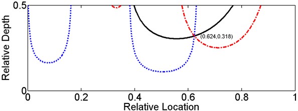
The three-contour method was validated using eigenfrequencies of the defective beam with a relative crack location 0.6 and a relative crack depth 0.3 provided above, as an instance. Fig. 5 shows three curved surfaces calculated via the three sub-equations in Eq. (19). The - and y-axes represent relative crack location and depth, respectively. The -axis in Fig. 5(a), (b) and (c) represent , and , respectively. For the conditions 0.6 and 0.3, 6.07, 2.81 and 17.07. The corresponding contours are projected onto the - plane and shown in Fig. 6, as the solid line, dotted line and dash dotted line, respectively. The contours intersect in the point 0.624 and 0.318. The relative errors are 4 % and 6 %, respectively, which denote a high precision of the proposed method.
Actually, the three contours are generally impossible meet in an exact point. It’s more frequent that each pair of contours intersect and finally three intersection points generate a triangle. Therefore, commonly, the triangular geometric center is selected as the intersection point of the three contours.
4. Experimental Illustration
Experiments were conducted to demonstrate the proposed algorithms. An uncracked and two cracked aluminum cantilever beams were manufactured with the same dimensions of 270 mm×10 mm×10 mm and material properties. An artificial single notch crack was made on each defective beam by wire-cutting technique with the relative depth 0.4. The crack on one beam is at position of 108 mm to the clamping end and the other is 189 mm, which means that the crack location e are respective 0.4 and 0.7.
The shock test was implemented to determine the first three eigenfrequencies of each cantilever beam. A pendulum applied a shock excitation to the beam at the position of 10 mm from the free end, and a self-synchronizing multipoint laser Doppler vibrometer [24] was employed to measure the out-of-plane surface displacement variation of four sampling points on the beam, as shown in Fig. 7. Laser Doppler vibrometer is a non-contact measurement tool, applying no accessional mass and influence to the specimen. When the pendulum almost hit the beam, the vibrometer was triggered to record the out-of-plane displacement, from the spectrum of which the first three eigenfrequencies of the corresponding beam can be extracted [24]. In order to eliminate error, an average value of eigenfrequencies obtained from the four sampling points was applied to the crack parameter calculation. All the measured eigenfrequencies and calculated crack parameters are shown in Table 3. Relative errors are computed and tabled, as well.
Fig. 5Variation curved surface of fc2/fc1, fc3/fc2, fc3/fc1 versus relative damage location and depth
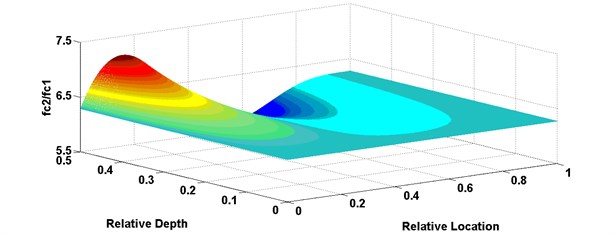
a)
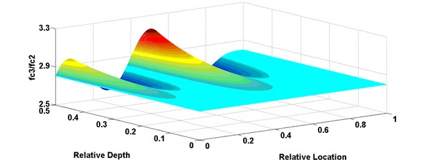
b)
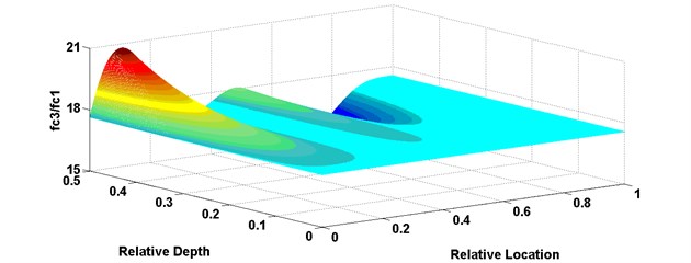
c)
Fig. 6Contours and their intersection under the damage conditions e= 0.6 and α= 0.3
Errors in the experiment are relatively larger than that in the numerical simulation. It is generally believed that the main error source is the difference between the real structure and its theoretical mathematic model based on the theory of Euler-Bernoulli beam and the rotational spring approximation of the crack damage. The difference brings forth an inherent error in the algorithm. The FEM model itself is established on the theory of Euler-Bernoulli beam, hence in numerical simulation this error is reduced. On the other hand, although a non-contact optical metrology method is adopted, the experimental setup induced measurement error is still inevitable. However, the relative errors in the experiments are less than 20 %, which can be accepted in engineering applications.
Fig. 7Experimental layout for the measurement of eigenfrequencies of a cantilever beam by LDV
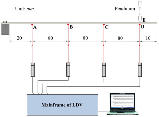
Table 3Eigenfrequencies of test beams and damage parameters calculated by the proposed two methods
Intact | 0.4 | 0.7 | |
1st eigenfrequency | 105.6 | 103.3 | 105.4 |
2nd eigenfrequency | 663.6 | 637.7 | 646.8 |
3rd eigenfrequency | 1865.7 | 1813.2 | 1735.9 |
calculated by Eq. (14) | – | 0.41 | 0.68 |
Relative error | – | 2.5 % | 2.85 % |
calculated by Eq. (11) | – | 0.37 | 0.33 |
Relative error | – | 7.5% | 17.5 % |
calculated by Eq. (19) | – | 0.41 | 0.74 |
Relative error | – | 2.5 % | 5.7 % |
calculated by Eq. (19) | – | 0.34 | 0.37 |
Relative error | – | 15 % | 7.5 % |
5. Conclusions
The location and the severity of a structural damage can be assessed by the change of eigenfrequency before and after the damage occurrence. Cantilever beam is one of the mostly common used structure types in engineering fields. In this paper, two eigenfrequency-based methods are developed to identify the damage location and severity of a cantilever beam. One is based on the eigenfrequency variation before and after the damage appearance, and the other is a three-contour method based on eigenfrequencies of the defective beam only. Both the two methods enjoy the virtue of demanding no knowledge of material characteristics of the structure. The three-contour method is less precise but more universal than the eigenfrequency-variation-based method, since it needs no frequency of the healthy structure. The uniqueness of solution is analyzed and confirmed, and numerical simulative and experimental verifications are carried out to show that the proposed methods are simple, effective and accurate.
References
-
Doebling S., Farrar C., Prime M., Shevitz D. Damage Identification and Health Monitoring of Structural and Mechanical Systems from Changes in Their Vibration Characteristics: a Literature Review. Los Alamos National Laboratory Report, LA-13070-MS, 1996.
-
Sohn H., Farrar C., Hemez F., Shunk D., Shevitz D, Nadler B. A Review of Structural Health Monitoring Literature. Los Alamos National Laboratory Report, LA-13976-MS, 2003.
-
Cruz P., Salgado R. Performance of vibration-based damage detection methods in bridges. Computer-aided Civil and Infrastructure Engineering, Vol. 24, Issue 1, 2009, p. 62-79.
-
Fan W., Qiao P. Vibration-based damage identification methods: a review and comparative study. Structural Health Monitoring, Vol. 10, Issue 1, 2011, p. 83-111.
-
Adams R., Cawley P., Pie C., Stone, B. A vibration technique for non-destructively assessing the integrity of structures. Journal of Mechanical Engineering Science, Vol. 20, Issue 2, 1978, p. 93-100.
-
Papadopoulos C., Dimarogonas A. Coupled longitudinal and bending vibrations of a rotating shaft with an open crack. Journal of Vibration and Control, Vol. 117, Issue 1, 1987, p. 81-93.
-
Rizos P., Asgragathos N., Dimarogonas A. Identification of crack location and magnitude in a cantilever beam from the vibration modes. Journal of Sound and Vibration, Vol. 138, Issue 3, 1990, p. 381-388.
-
Ostachowicz W., Krawczuk M. Analysis of the effect of cracks on the natural frequencies of cantilever beam. Journal of Sound and Vibration, Vol. 150, Issue 2, 1991, p. 191-201.
-
Liang R., Choy F., Hu J. Detection of cracks in beam structures using measurements of natural frequencies. Journal of the Franklin Institute-Engineering and Applied Mathematics, Vol. 328, Issue 4, 1991, p. 505-518.
-
Nandwana B., Maiti S. Detection of the location and size of a crack in stepped cantilever beams based on measurements of natural frequencies. Journal of Sound and Vibration, Vol. 203, Issue 3, 1997, p. 435-446.
-
Chaudhari T., Maiti S. A study of vibration of geometrically segmented beams with and without crack. International Journal of Solids and Structures, Vol. 37, Issue 5, 2000, p. 761-779.
-
Owolabi G., Swamidas A., Seshadri R. Damage detection in beams using changes in frequencies and amplitudes of frequency response function. Journal of Sound and Vibration, Vol. 265, Issue 1, 2003, p. 1-22.
-
Cawley P., Adams R. The location of defects in structures from measurements of natural frequencies. Journal of Strain Analysis, Vol. 14, Issue 2, 1979, p. 49-57.
-
Hearn G., Testa R. Modal analysis for damage detection in structures. Journal of Structural Engineering, Vol. 117, Issue 10, 1991, p. 3042-3062.
-
Narkis Y. Identification of crack location in vibrating simply supported beams. Journal of Sound and Vibration, Vol. 172, Issue 4, 1994, p. 549-558.
-
Gudmundson P. Eigenfrequency changes of structures due to cracks, notches or other geometrical changes. Journal of the Mechanics and Physics of Solids, Vol. 30, Issue 5, 1982, p. 339-353.
-
Kim J., Stubbs N. Crack detection in beam-type structures using frequency data. Journal of Sound and Vibration, Vol. 259, Issue 1, 2003, p. 145-160.
-
Kim J., Ryu Y., Cho H., Stubbs N. Damage identification in beam-type structures: frequency-based method vs mode-shape-based method. Engineering Structures, Vol. 25, Issue 1, 2003, p. 57-67.
-
Rubio L. An efficient method for crack identification in simply supported Eular-Bernoulli beams. Journal of Vibration and Acoustics, Vol. 131, Issue 5, 2009, p. 051001.
-
Sayyad F., Kumar B. Identification of crack location and crack size in a simply supported beam by measurement of natural frequencies. Journal of Vibration and Control, Vol. 18, Issue 2, 2012, p. 183-190.
-
Sayyad F., Kumar B. Theoretic al and experimental study for identification of crack in cantilever beam by measurement of natural frequencies. Journal of Vibration and Control, Vol. 17, Issue 8, 2011, p. 1235-1240.
-
Sayyad F., Kumar B. Approximate analytical method for damage detection in beam. International Journal of Damage Mechanics, Vol. 21, Issue 7, 2012, p. 1064-1075.
-
Chondros T., Dimarogonas A., Yao J. A continuous cracked beam vibration theory. Journal of Sound and vibration, Vol. 215, Issue 1, 1998, p. 17-34.
-
Yang C., Guo M., Liu H., Yan K., Xu Y., Miao H., Fu Y. A multi-point laser Doppler vibrometer with fiber-based configuration. Review of Scientific Instruments, Vol. 84, Issue 12, 2013, p. 121702.
About this article

The authors would like to acknowledge the financial support provided by the National Science Foundation of China (NSFC) under Grant No. 11502257, the key subject “Computational Solid Mechanics” of CAEP, and the Science and Technology Development Foundation of CAEP under Grant No. 2014B0101009.
