Fault diagnosis of rolling bearing under complex working conditions based on time-frequency joint feature extraction-deep learning

1. Introduction

Rolling bearing is one of the key components of kinds of machinery, and its degradation and damage will have a significant impact on the performance and life of the entire machine system [1]. In recent years, most of relevant studies are under the assumption of constant working conditions, and their effects will be reduced greatly under complex working conditions such as varying speed, varying loading, strong noise inference and so on [2]. Therefore, it is of great significance to ensure the normal operation of mechanical equipment by studying the intelligent fault diagnosis method under the above-mentioned complex work conditions. Currently, the solution to the above problem usually focuses on two directions: 1) Feature extraction based on time-frequency analysis method. 2) Intelligent algorithm for subsequent classification by using the extracted features.

In the past decades, kinds of time-frequency feature extraction methods such as empirical mode decomposition (EMD), short-time Fourier transform (STFT) and variational mode decomposition (VMD) and so on have been used widely in fault diagnosis due to the reason that they could reflect the fault characteristics in time and frequency simultaneously [3-6]. Bao proposed a new time-frequency analysis method, which can adapt to the change of STFT based on fast path optimization, and the proposed new time-frequency analysis method is used in fault diagnosis of planetary gearboxes successfully [7]. The correlation coefficient characterization method is used to obtain the sensitivity of each IMF obtained by EMD, then signal is reconstructed by using the obtained sensitive IMFs to remove noise, finally fault diagnosis of shearer rocker in strong noise environment is realized by using the reconstructed signal [8]. Unfortunately, there exists inherent defects in STFT and EMD: the diagnosis effect of STFT is related closely to its window width, but the window width is usually fixed and cannot be adjusted adaptively. The modal aliasing phenomenon of EMD is inevitable, which affects the decomposition result to some extent. VMD is a relative new time-frequency processing method proposed in recent years, which could decompose the analyzed signal into multiple single-component amplitude modulation signals at one time, and the above defects encountered by STFT and EMD could be avoided by VMD [9]. Ding proposed a VMD algorithm based on variable particle swarm optimization parameters for nonlinear and nonstationary problems [10]. Similarly, Wang also proposed a new genetic algorithm to optimize the parameters of VMD, and the accuracy and robustness of the proposed VMD were improved greatly in the diagnostic area [11]. Though the use of VMD has achieved good results in feature extraction, the extracted features only contain characteristics in one single aspect, which is often insufficient in reflecting the fault state, and the phenomenon is especially severe in complex work condition [12], so this paper attempts to use VMD for fault feature extraction in three aspects (time domain, frequency domain and time-frequency domain) simultaneously.

After extracting features from vibration signals, intelligent algorithms are often used as the carrier to create a solid fault classification model. From the end of the last century to the beginning of this century, there are three kinds of intelligent algorithm classification models: models based on rich experience and knowledge, models based on corresponding statistical analysis, modes based on shallow machine learning algorithms such as random forest, support vector machine, K-nearest neighbor algorithm and so on [13-19]. However, the above mentioned three models have the defects of requiring rich professional knowledge or complex mapping relationships. Besides, their language expression abilities are very limited, and there are also different distribution of training and test data. With the rapid development of deep learning, it has been used widely in fault diagnosis in recent years, which could explore the mapping relationship between the vibration signals or extracted feature and the corresponding fault types more precisely. The extracted two-dimensional images removing the influence of handmade features are used as input of LeNet-5 to achieve a high recognition rate successfully [20]. The spectral coefficient and wavelet characteristic values of the vibration signal are extracted and input into the deep confidence network model to obtain a relative satisfactory diagnostic effect [21]. The advantages of LSTM network and statistical process analysis are combined and a LSS model is proposed for aero-engine bearing performance degradation prediction [22].To solve the difficulty in fault feature extraction of rolling bearing under complex working conditions and inspired by the above-mentioned deep learning literatures, a fault diagnosis method of rolling bearing under complex working conditions based on time-frequency joint feature extraction-deep learning is proposed. The main contributions of the study include the following aspects:

1) A time-frequency feature extraction method based on VMD is proposed to address the shortcomings of traditional time-frequency analysis methods such as STFT and EMD mentioned above. Furthermore, based on the proposed time-frequency extraction method, time-domain, frequency-domain and time-frequency domain feature extraction vectors are formed to effectively solve the problem of key feature information loss caused by a single time-domain ore frequency-domain feature vector, thereby providing a basic guarantee for improving subsequent classification accuracy.

2) A hybrid deep learning model named SAM-RNN-DCNN is constructed by combining sparse attention mechanism (SAM), recurrent neural network (RNN) with convolutional neural network (CNN) using their respective advantages, and the constructed model has the advantages of reducing the complexity of training data, increasing the interdependence among sequences and having high diagnostic accuracy.

3) The advantages of the proposed time-frequency feature extraction method and the proposed hybrid deep model (SAM-RNN-DCNN) are combined to solve the fault diagnosis problem under variable speed, variable load and strong noise interference. Corresponding experiments are carried out to show the wonderful performance of the proposed method.

4) Comparisons are also carried out to verify the advantages of the proposed method over the other related methods.

2. Theoretical basis

2.2. Recurrent neural network (RNN)

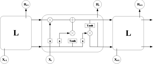
The dynamic temporal behavior and related remote dependencies of the input sequences could be captured by RNN. Besides, the correlations between sequences also could be enhanced by RNN and the output of neurons can directly act on itself in the next time frame [25], which makes RNN have strong memory capabilities. However, RNN has the problem of gradient vanish [26]. In order to solve this problem, the long short-term memory recurrent neural network (LSTM-RNN) was derived, which is a variant of RNN and can solve the problem of gradient disappearance perfectly, so it has been used widely in fault diagnosis. The architecture of LSTM-RNN is shown in Fig. 1.

The LSTM-RNN network structure is generally composed of three gates: the forget gate, the input gate, and the output gate [25].The math expressions of these three gates are as follows:

5

$\left\{\begin{array}{l}{f}_t=\sigma \left(w_f*\left[H_{t-1},X_t\right]+b_f\right),\\ i_t=\sigma \left(w_i*\left[H_{t-1},X_t\right]+b_i\right),\\ \widehat{C_t}=\mathrm{t}\mathrm{a}\mathrm{n}\mathrm{h}\left(W_c*\left[H_{t-1},X_t\right]+b_c\right),\\ C_t=f_t*C_{t-1}+i_t*\widehat{C_t},\\ o_t=\sigma \left(W_O*\left[H_{t-1},X_t\right]+b_o\right),\\ H_t=o_t*\mathrm{t}\mathrm{a}\mathrm{n}\mathrm{h}\left(C_t\right),\end{array}\right.$

where, $C_t$ represents the calculation method of the storage unit of $t$ time. $H_t$ represents all the output points of the storage cell of time $t$. $W$ and $b$ are the coefficient matrix and bias vector, and $\sigma$ is the activation function. $i$, $f$ and $o$ are the calculation method of the three gates of $t$ time point.

Fig. 1LSTM-RNN architecture

2.3. Convolutional neural network (CNN)

CNN is one of feedforward neural networks with the advantages of local cognition, shared weight values, and down sampling in space and time, which usually consists of multiple convolutional levels performing feature extraction tasks and one single output stage of combined extraction of advanced features to predict the desired output [27]. Fig. 2 shows a simple CNN architecture. Generally, CNNs have the ability of reducing the number of parameters through convolution, and can also handle the mapping relationship between signal and fault type effectively [28]. Many different network structures have been developed to make them more suitable for diagnosis in various situations with continuous development. However, most of these CNN structures are composed of the following modules.

Fig. 2Basic architecture of CNN

Convolutional layer: the convolutional layer consisting of multiple feature maps can learn the features of the input data. Neurons in one feature map are mainly connected to local areas of the previous function map by a set of weights [29]. The calculation of convolutional layer can be expressed by Eq. (6):

6

${\chi }_j^n=f\left({\sum }_{i\in M_j}^{}{X}_i^{I-1}*k_{ij}^I+b_j^i\right),$

where $X_i^{I-1}$ is the $j$ feature in layer $I-1$, $M$ and $k$ represent the input feature set and convolution kernel respectively. $f(.)$ and $b$ represent the nonlinear activation function and bias term respectively.

Pooling layer: the pooling layer is typically located between two consecutive convolutional layers. It is used to reduce the dimensionality of the convolutional layer for the purpose of feature extraction. Depending on the application, the pooling tier can be maximum pooling or average pooling. The calculation process for its maximum pooling is shown in Eq. (7):

7

$x_j^{l+1}=p\left(x_j^l\right),$

where $x_j^{l+1}$ is the $j$ characteristic of layer $l+1$, and $p\left(x_j^l\right)$ represents pooling operations in the network.

Fully connected layer: its role is mainly to extend the output of the last pooled layer into a one-dimensional feature vector and input into the follow fully connected layer. The relevant calculations can be shown in Eq. (8):

8

$x^l=f\left(w^l{x}^{l-1}+b^l\right),$

where $w^l$ and $b^l$ represent the weight and bias values of the fully connected layer respectively.

SoftMax: SoftMax is a generalization of Logistic functions to multidimensionality. SoftMax sums the vectors of $k$ real values to 1. The input of SoftMax can be positive, negative, zero, or greater than 1, and SoftMax converts the input between 0 and 1, so it can be used for multi-class classification. The mathematical equation for SoftMax can be represented by Eq. (9):

9

$\sigma (\overrightarrow{z}{)}_i=\frac{e^{zi}}{{\sum }_{j=1}^k{e}^{zi}},$

where $\overrightarrow{z}$ is the input vector of SoftMax, $e^{zi}$ is the standard exponential function being applied on each element of the input vector, and $k$ is the number of classes in the multiclass classification.

2.4. Sparse attention mechanism (SAM)

SAM was first proposed in literature [30], which can learn both local characteristics and long-range sparse correlations [31], SAM has been gradually applied on fault diagnosis owing to its unique advantages. Fig. 3 shows the schematic of a general SAM.

Fig. 3SAM schematic

The SAM presented in reference [32] is used in this article, which has strong effectiveness in improving diagnostic accuracy and expanding the receptive field without adding more convolutional layers, and has better performance in processing longer sequences. This attention mechanism uses latent variables to learn the most relevant features, allowing visualization of the most important timestamps for each instance to facilitate understanding and interpretability of the output results. Furthermore, SAM can improve attention while reducing the complexity of data. The parameter in SAM has only one $\alpha$ (sparsity coefficient), which is defined in Eq. (10):

10

${\alpha }_t-T_l:t-1=\alpha -en{t}_{\mathrm{m}\mathrm{a}\mathrm{x}}\left(h_{t-T_l:t-1}\cdot h_t^T\right)=\mathrm{R}\mathrm{e}LU\left(\left(\alpha -1\right)\times \left(h_{t-T_l:t-1}\cdot h_t^T\right)-\tau 1\right){)}^{\frac{1}{\alpha }-1},$

where $\tau$ is the Lagrange multiplier, $\alpha -en{t}_{\mathrm{m}\mathrm{a}\mathrm{x}}$ maps the latent variable to a sparse attention score ${\alpha }_{\mathrm{t}}-T_l:t-1\in {\mathfrak{R}}^{T_l\times 1}$, which is mainly based on the point-multiplied similarity $h_{t-T_l:t-1}\in {\mathfrak{R}}^{T_l\times d_{hid}}$ between historical steps and the current step size $h_t\in {\mathfrak{R}}^{1\times d_{hid}}$, and $1$ refers to the vector. $\mathrm{R}\mathrm{e}LU\mathbb{k}$ is the activation function.

3. Time-frequency joint feature extraction and hybrid deep learning diagnostic model based on VMD decomposition

Addressing the issue of low diagnostic accuracy due to insufficient features under variable operating conditions, a fault diagnosis model based on VMD decomposition combining feature extraction with hybrid deep learning is proposed, which not only solves the problem of insufficient extracted fault feature in diagnosis process, but also has high diagnostic accuracy. The specific diagnostic process is shown in Fig. 4, and its details are as follows.

Fig. 4Diagnostic flowchart

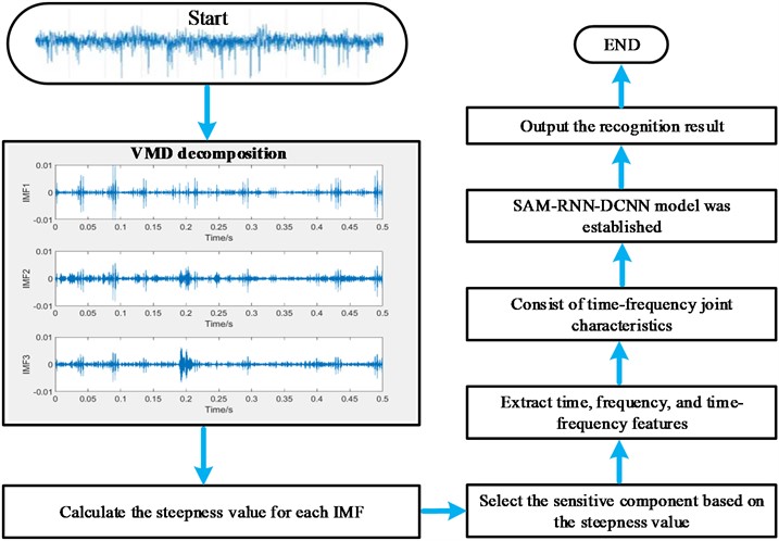
Step 1: collect the vibration data of rotating machinery under different running states.

Step 2: apply VMD analysis on the collected vibration data and several IMFs are obtained.

Step 3: to extract sensitive features and eliminate noise interference, the steepness values of the obtained IMFs are calculated and the IMF with biggest steepness value are selected for subsequent handling.

Step 4: the time-domain, frequency-domain and time-frequency domain features are extracted based on the selected IMF to avoid the problem of key feature information loss caused by a single time-domain ore frequency-domain feature vector, thereby providing a basic guarantee for improving subsequent classification accuracy.

Step 5: construct the hybrid deep learning model (SAM-RNN-DCNN) through combining sparse attention mechanism (SAM), recurrent neural network (RNN) with convolutional neural network (CNN) using their respective advantages to reduce the complexity of training data, increase the interdependence among sequences and increase diagnostic accuracy.

Step 6: divide the feature vectors obtained in step 4 into training and test parts: the training parts are used to train the constructed hybrid deep learning model and the test parts are input into the trained model to get classification results.

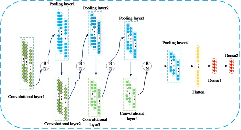
In this hybrid model, ReLU is used as the activation function and maximum pooling operation. The BN layer is added after the convolutional layer, which helps to improve the domain adaptability and generalization of the model. It is found that the effects of four-layer convolutional layer and five-layer convolutional layer are the same through experimental comparison, so the four-layer convolutional layer is selected to reduce the depth of the convolutional layer, and the results of the experiment are shown in Table 1. Furthermore, two fully connected layers are adopted: Dense 1 is used mainly to map the abstract information in the different sizes of the receptive field learned by the previous convolutional layer to a larger space, increasing the characterization ability of the model. Dense2 is used mainly to match the output scale of the signal detection network. The specific structure of the used CNN part in the paper is shown in Fig. 5.

Fig. 5The specific structure of the used CNN

The proposed hybrid model naming SAM-RNN-DCNN comprehensively utilizes the advantages of SAM in improving diagnostic accuracy, RNN’s strong network memory and CNN’ high computational efficiency. The model is mainly composed of four modules: SAM module, RNN module, CNN module, and connection output module. A dropout layer is also added to the model,which can alleviate the overfitting phenomenon effectively [33]. The SAM-RNN-DCNN model is shown in Fig. 6.

3.1. Hyperparameter settings

The accuracy of diagnosis is closely related to the setting of hyperparameters, which not only affects the speed of diagnosis, but also has a significant impact on the stability and accuracy of diagnosis [34]. In this paper, the Adam optimizer is used, which can introduce both momentum and adaptive learning rate to accelerate convergence, so that the corresponding weights can converge to the optimal interval much faster. The learning rate determines whether the objective function can converge to the local minimum and the time it converges to the minimum. Momentum affects the direction of gradient descent, and the appropriate momentum size helps to accelerate or decelerate the gradient change of the base learning rate relative to the network. In this article, the size of the learning rate is 0.00001 and the size of the momentum is 0.9 based on experience. The main hyperparameters used in this article are presented in Table 2.

Fig. 6SAM-RNN-DCNN hybrid model

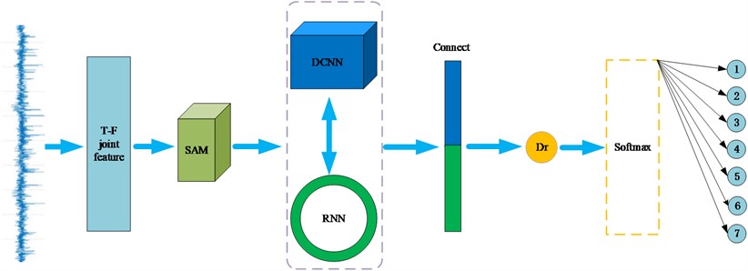
Table 2Hyperparameter settings

No.	Layer type	Kernel number	Kernel size	Kernel stride
1	Batch size	32	/	/
2	Epoch	100	/	/
3	Conv1d_1	16	64×1	2×1
4	Conv1d_2	32	5×1	2×1
5	Conv1d_3	64	3×1	2×1
6	Conv1d_4	64	3×1	2×1
7	Every MaxPooling1D	64	2×1	2×1
8	Dropout	1	0.5	/
9	Dense1	1	200	/
10	Dense2	1	100	/

4. Experimental verification

Two types of experimental data representing the complex work conditions of time-varying speed and time-varying loading respectively are selected to verify the effectiveness of the proposed method. Besides, the robustness to noise of the proposed method is verified by adding different degree of noise into the vibration signals.

4.1. Experimental verification under variable rotational speed working condition

The accuracy of the diagnostic model for diagnosing bearing faults under different speed scenarios is a very important indicator of the diagnostic performance of the model [35]. In order to verify the diagnostic performance of the proposed model under different speeds, the bearing dataset of the University of Ottawa in Canada was selected, which contains the vibration signals collected from bearings with different fault types under time-varying speed conditions. All data were collected on the test bench as shown in Fig. 7, where the bearing type used is ER16K, and the specific parameters of the bearing are shown in Table 3. The data set includes three kinds of fault: normal, inner ring fault, and outer ring fault. Each fault type contains four states in which the speed is continuously raised, decreased, raised and then decreased, decreased and then raised. The changes of the rotational speed are shown in Fig. 8. A total of 36 datasets are collected, all of which were sampled at 200 kHz with a sampling duration of 10 seconds.

Table 3Test bench bearing parameters

Type	Number of balls	Pitch diameter	Ball diameter	Bearing FCCo	Bearing FCCI	Diameter ratio of sheaves	Number of gear teeth
ER16K	9	38.52 mm	7.94 mm	3.57	5.43	1:2.6	18

Fig. 7Bearing test bench

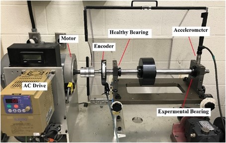
Fig. 8The fours state of time-varying rotational speed

a) The rotational speed is always increasing

b) The rotational speed is constantly decreasing

c) The rotational speed is increasing and then decreasing

d) The rotational speed is decreasing and then increasing

The original time-domain waveforms of the four time-varying speed conditions corresponding to the three fault states are plotted in Fig. 9.

Fig. 9Time domain waveforms under variable speed

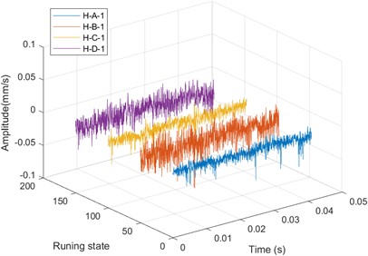
a) Four conditions s under normal

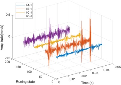
b) Four conditions with inner ring failure

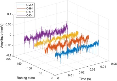
c) Four conditions with outer ring failure

7 different data sets are selected, and their IMF components as shown in Fig. 10 are obtained after VMD decomposition. The fault information sensitive IMF component is selected by comparing the steepness values of each IMFs. The three conditions with rotational speed being always increasing are taken as examples, and their corresponding time-frequency diagram as shown in Fig. 11. The time-domain domain, frequency domain and time-frequency domain features are extracted to form time-frequency joint features and used as input of the established SAM-RNN-DCNN hybrid deep learning model for fault diagnosis.

Fig. 10VMD decomposition

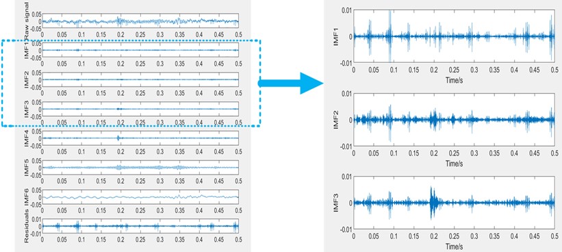
Fig. 11Time-frequency diagrams of the three conditions with rotational speed being always increasing

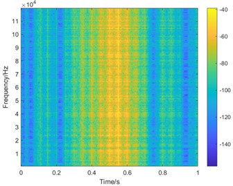
a) Time-frequency diagram of healthy bearing with always increasing speed

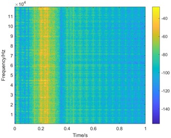
b) Time-frequency diagram of inner race faulty bearing with always increasing speed

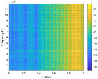
c) Time-frequency diagram of outer race faulty bearing with always increasing speed

The ACC and Loss curves as shown in Fig. 12 of the diagnostic hybrid model are obtained after 100 iterations, and it could be observed that a high accuracy rate of 99.7% and fast convergence ratio could be obtained by the proposed method. Besides, the hybrid model has the advantages of perfect stability and no overfitting.

Fig. 12Training and validations acc and loss graphs

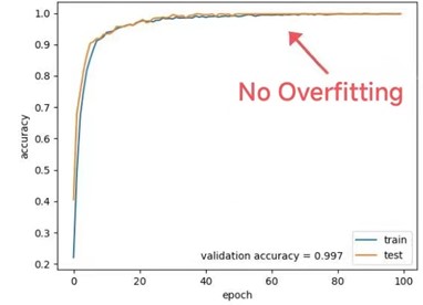
a) Accuracy

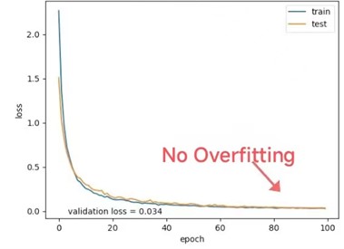
b) Loss

Fig. 13Confusion matrix diagram

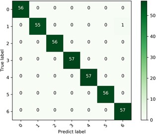
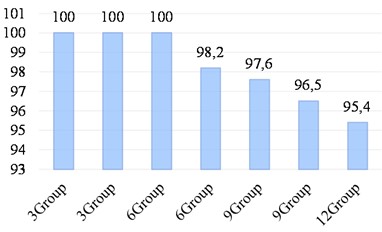
Fig. 14Accuracy rate by situation

In the experiment, 7 types of fault categories are selected, and the excellent performance of the proposed model can be seen intuitively by drawing the confusion matrix as shown in Fig. 13.

3, 6, 9 and 12 groups of preprocessed data sets with different fault types under different rotational speeds are selected respectively to verify the generalization of the proposed hybrid model, and the generalization verification result is presented in Fig. 14, based on which it can be seen that the accuracy of identifying faults is more than 95 %. It is verified that the hybrid model has strong robustness to variable rotational speed.

4.2. Experimental verification of variable load conditions

CWRU dataset is one of the most commonly used datasets, and the test bench with its structure diagram are given in Fig. 15 [36]. The bearing data set under 0 HP, 1 HP, 2 HP, 3 HP load (1 HP = 0.746 KW) are selected to verify the proposed method’ robustness to variable load (Note: all the data set is collected under sampling frequency 12 kHz), and the speeds corresponding to each load are shown in Table 4. The data set is divided into four fault types: normal, inner ring fault, outer ring fault and ball failure, which can be further subdivided into 10 fault types as shown in Table 5 according to the fault’ severity.

Fig. 15The test bench with its schematic diagram

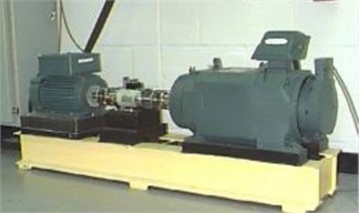
a) Bearing test bench

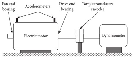
b) Schematic diagram of the structure

Table 4The speeds corresponding to each load

Dataset	Motor load	Shaft speed
A	0 Hp	1797 Rpm
B	1 Hp	1772 Rpm
C	2 Hp	1750 Rpm
D	3 Hp	1730 Rpm

Table 510 types of faults

Fault ID	Fault Cause	Severity
1	Normal	N/A
2	Inner race fault	0.007 inch
3	Ball fault	0.007 inch
4	Outer race fault	0.007 inch
5	Inner race fault	0.014 inch
6	Ball fault	0.014 inch
7	Outer race fault	0.014 inch
8	Inner race fault	0.021 inch
9	Ball fault	0.021 inch
10	Outer race fault	0.021 inch

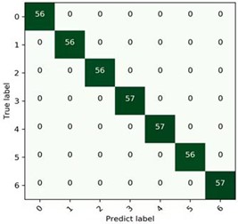
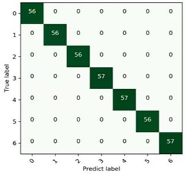
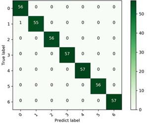
In the experiment, 7 different fault types of data sets under four different loads from0-3HP were selected separately, and they are processed by the proposed feature extraction process, then are fed into the hybrid deep learning model for fault classification. The form and accuracies of the corresponding confusion matrixes as shown in Fig. 16 are used to verify the excellence of the proposed model under variable load condition.

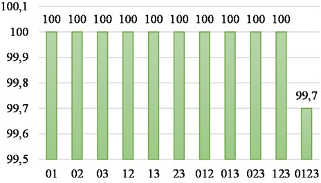
In order to further verify the generalization of the proposed model under different loads, two combinations and three combinations were randomly selected under 0-3 HP loads, and the experimental results were shown in Fig. 17. It can be seen that except for the accuracy of 99.7 % under the four loads, the diagnostic accuracies of the rest are 100 %, which fully verifies that the proposed method has strong generalization virtue under different loads.

Fig. 16Confusion matrix diagram under each load

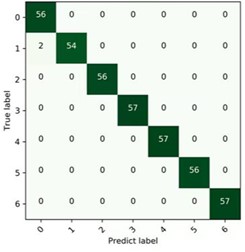
a) 0 HP

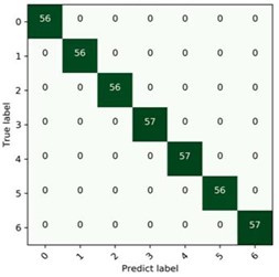
b) 1 HP

c) 2 HP

d) 3 HP

e) 0-3 HP

Fig. 17Accuracy in each case

5. Comparative experiments

In the section, the RNN, DCNN and RNN-DCNN models are used for comparison. The data set in section 3 are processed using the proposed feature extraction method same as section 3, then the extracted features are input into the above three models, and the iterations of the training models is 100. The corresponding last classification results of the four deep learning models are presented in Fig. 19, based on which the high accuracy of the proposed method is evident. Besides, it was found that there existed overfitting phenomenon in the RNN, DCNN and RNN-DCNN models, but not in the proposed SAM-RNN-DCNN hybrid model.

Fig. 18Accuracy at each signal-to-noise ratio

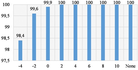
Fig. 19Comparative test under variable load

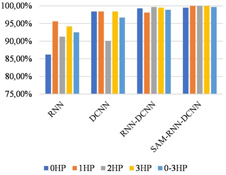
Fig. 20Comparative test under variable rotational speed

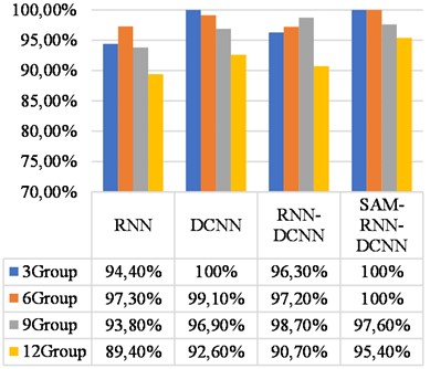
The second comparison experiment uses the dataset under variable speed same as section 3.1: 3, 6, 9 and 12 groups of data set are set and the feature extraction are same. The extracted features are input into the RNN, DCNN and RNN-DCNN models and the last comparison results are given in Fig. 20, based on which the advantage of the proposed model over the other three models are is further verified.

6. Discussion

The experimental results of three case studies (time varying speed, time-varying loading and strong noise inference) show that the proposed method exhibits excellent classification performance in two different experiments. The emergence of this result is due to our consideration of the fact that bearings often operate at complex situation and are susceptible to time-varying conditions and strong noise interference in actual operation. Therefore, we propose one combined method to tackle the difficulty. By integrating time-frequency feature extraction method based on VMD with one constructed hybrid deep learning model, the classification performance of the model under time-varying speed, time-varying load and strong noise interference has been improved. For the experimental dataset of case 1, that is under time-varying speed situation, the accuracy of the proposed method is more than 95 %. Besides, the accuracy is almost unaffected by the number of test vectors. As for the experimental of case 2, that is under time-varying load situation, the accuracy under the four different loads is 99.7 %, and the diagnostic accuracies of the rest are 100 %. For the experimental dataset of case 3, that is under strong noise inference, the proposed method is about 5 % higher than the other related methods. It is worth noting that compared to traditional processing methods, this method is more intelligent, efficient, and has better generalization performance. In addition, we mainly use single vibration signals without the need for additional tachometers or human intervention, and can still meet diagnostic requirements under strong noise interference.

7. Conclusions

Aiming at solving the problem of insufficient fault information based on single domain and the low diagnostic accuracy under complex time-varying working conditions, an intelligent fault diagnosis method based on time-frequency joint feature extraction-deep learning is proposed. The proposed method takes advantage of VMD’ virtue in handling nonlinear and non-stationary vibration signals, and the problem of insufficient fault information relying on single domain could be solved to great extent. One hybrid deep learning model naming SAM-RNN-DCNN is proposed, which comprehensively combines the advantages of SAM, RNN and DCNN and could realize high-precision fault diagnosis.

Effectiveness of the proposed is verified thorough the experiments under three complex work conditions (time-varying speed condition, time-varying loading condition and strong background noise). Besides, the advantage of the proposed method over the other three related models, that is RNN, DCNN and RNN-DCNN is also verified. In all, the proposed method has strong stability, generalization and noise robustness under complex working conditions.

Up to now, the proposed method is only effective in fault diagnosis of rotating machinery when single fault arises, and its use in compound fault diagnosis of rotating machinery is our future work.