Abstract
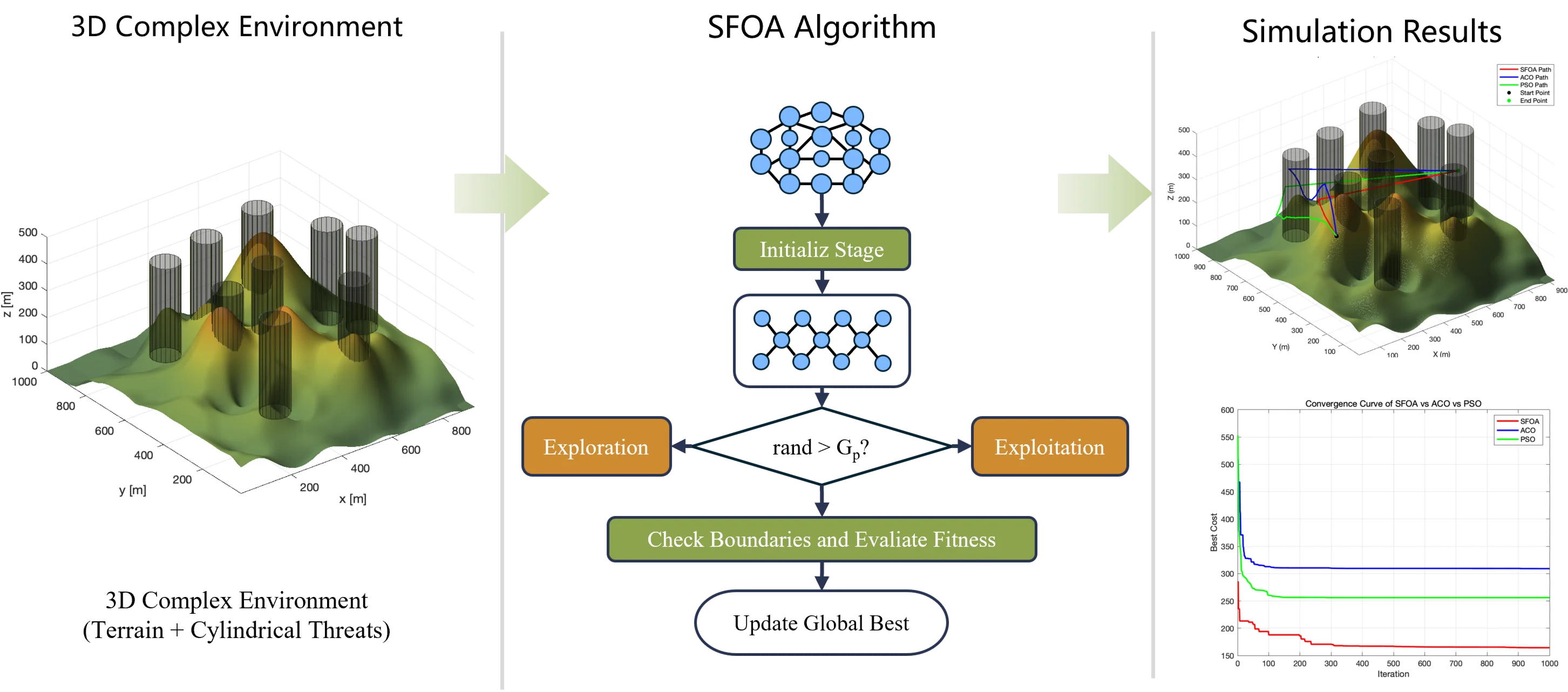
When solving the path planning problem for Unmanned Aerial Vehicle (UAV) in a three-dimensional complex environment, traditional algorithms often face issues like falling into local optimum easily, insufficient global search ability, poor efficiency and defective optimization result. To address these issues, a three-dimensional path planning method is proposed based on the Starfish Optimization Algorithm (SFOA). This algorithm, inspired by the exploration, preying, and regeneration behaviors of starfish, balances global search and local exploitation, enhancing UAV trajectory planning in complex environments. The study constructs a complex three-dimensional environment model and designs a comprehensive optimization objective by covering constraints like trajectory length, safety, flight height, and smoothness. The trajectory planning framework proposed in this study is designed for pre-mission planning, generating UAV paths offline based on known static terrain and threat information. Comparative experimental results with Ant Colony Optimization and Particle Swarm Optimization show that the SFOA-based UAV trajectory planning achieves significant improvements in comprehensive cost and convergence speed, demonstrating superior global optimization performance. This offers an innovative solution for UAV efficiently and safe trajectory planning in complex environments.
Highlights
- Proposes a 3D UAV trajectory planning method based on the Starfish Optimization Algorithm (SFOA), addressing the limitations of traditional algorithms such as easy local optima and insufficient global search capability.
- Constructs a comprehensive multi-objective cost function integrating path length, obstacle avoidance safety, flight altitude constraints, and trajectory smoothness, ensuring feasible and optimal paths.
- SFOA balances global exploration (hybrid 5D/1D search) and local exploitation (predation-regeneration mechanism), adapting to high-dimensional complex optimization scenarios.
- Comparative experiments with ACO and PSO show SFOA reduces the best comprehensive cost by up to 46.84% (vs ACO) and 35.81% (vs PSO) in complex environments, with faster convergence speed.
1. Introduction
Unmanned aerial vehicles (UAVs), as emerging aerial vehicles, are becoming increasingly prevalent in military, civilian, and commercial sectors. However, trajectory planning remains a critical factor restricting their effectiveness. UAV trajectory planning aims to find the optimal flight path from the current position to the target position in each three-dimensional space while ensuring flight safety. In actual flights, UAVs' positions change constantly, and their operating environments are often highly complex. Therefore, flight paths must be optimized in real-time based on environmental conditions and mission requirements to handle uncertainties and avoid collisions. Given the complex flight constraints and dynamic environments, it is essential to develop constraint models and apply efficient optimization methods for solving.
In recent years, an increasing number of researchers have integrated UAV operation features and low-altitude flight environment characteristics to explore UAV trajectory planning using various algorithms [1], [2]. In complex environments, UAV trajectory planning faces multiple challenges, such as obstacle avoidance in uncertain terrains, threat region evasion, dynamic flight constraints including turning radius and climb angle limits, and the need for real-time path updates. Many classical methods, such as the A* algorithm [3], artificial potential field method [4], [5], and Voronoi diagrams [6], are extensively applied in path planning but are mainly suitable for two-dimensional space. For complex three-dimensional path planning, intelligent methods have gained considerable attention. Typical examples include genetic algorithms [7], artificial bee colonies [8], ant colony optimization [9], and particle swarm optimization [10], [11]. In UAV path planning, the ant colony algorithm stands out for its simple coding and effective optimization guidance [12]. Particle swarm optimization has also proven effective for UAV path planning in known static rough terrains, offering fast convergence, global optimization, and parallel search advantages [13].
In UAV path planning, ACO guides agents by combining pheromone trails and heuristic. Each UAV probabilistically selects the next waypoint according to the pheromone concentration and heuristic desirability, gradually reinforcing shorter and safer routes while weakening less efficient ones [14]. In addressing complex problems, the ant colony algorithm has drawbacks like slow convergence and low solution precision defined here as the residual gap between returned cost and the theoretical optimum; typical mitigations include hybridizing ACO with local 2-opt refinement or adaptive tuning of pheromone parameters. The particle swarm algorithm is sensitive to parameters and prone to local optima. To tackle these issues, meta-heuristic algorithms have emerged as an effective approach for complex optimization problems [15]. They can effectively avoid local optima, offering strong adaptability and robustness for handling diverse and complex optimization challenges. Three-dimensional intelligent methods refer to bio-inspired and heuristic optimization algorithms capable of handling multi-objective UAV path planning in complex 3D terrains. These include Genetic Algorithms (GA), Particle Swarm Optimization (PSO), Ant Colony Optimization (ACO), and Starfish optimization algorithm (SFOA).
Unlike Grey Wolf Optimization (GWO) and Whale Optimization Algorithm (WOA), which primarily relies on fixed encircling or spiral update patterns, the Starfish Optimization Algorithm (SFOA) combines five-dimensional hybrid exploration and adaptive regeneration mechanisms inspired by starfish arm coordination. This dual-phase search allows SFOA to balance exploration and exploitation more flexibly in high-dimensional spaces such as 3D UAV path planning. The Starfish Optimization Algorithm (SFOA) is a novel search strategy inspired by the exploration, foraging, and regeneration behaviors of starfish in nature, operating in two phases: exploration and exploitation. During the exploration phase, the selection between five-dimensional and one-dimensional search strategies is based on the number of optimization variables (nD). When nD > 5, a five-dimensional pattern ensures sufficient global exploration across multiple dimensions. When nD ≤ 5, the search space is narrower and requires more precision, so a one-dimensional search improves convergence accuracy and reduces redundant computation, it uses a hybrid search strategy combining five-dimensional and one-dimensional search patterns to boost computational efficiency while maintaining strong search capabilities. In the exploitation phase, the algorithm mimics the foraging and regeneration of starfish, employing bidirectional search and unique movement patterns to ensure effective convergence. Through extensive testing on benchmark functions and engineering problems, SFOA has shown remarkable advantages in solving global optimization problems [16].
Traditional path-planning algorithms, though effective for specific problems, still suffer from slow convergence, local optima, and high computational complexity when dealing with complex environments, multiple constraints, and multi-objective optimization. To address these issues, this paper proposes a UAV path-planning method based on the Starfish Optimization Algorithm. It leverages the bio-inspired characteristics of starfish foraging and regeneration to enhance the global search ability and local optimization precision in path planning.
The rest of this paper is structured as follows. Section 2 presents the modeling of UAV path planning. Section 3 explains the basic principle and characteristics of the SFOA. In Section 4, simulation verification of UAV path planning in complex environments using SFOA is carried out, in a complex environment with nine obstacles, SFOA reduced the best cost by up to 46.84 % and 35.81 % compared to ACO and PSO, respectively. In a simpler five-obstacle scenario, SFOA still achieved reductions of 45.52 % and 41.24 % over ACO and PSO. These results validate the efficiency and robustness of SFOA in multi-objective 3D path planning, offering an innovative and effective solution for safe and efficient UAV trajectory design in diverse and challenging environments. Finally, Section 5 offers conclusions and suggestions for future work.
2. Modeling of UAV path planning
2.1. Three - dimensional path constraint model for UAV
UAV path planning is a crucial task-execution step, aiming to plot a safe, feasible, and optimal route that meets mission requirements. In complex environments, this involves obstacle avoidance, threat evasion, and considering flight altitude, path smoothness, and maneuverability constraints. This paper develops a 3D path maneuverability constraint model [17], which transforms path planning into a multi-constraint optimization problem via a comprehensive cost function.
The UAV path-planning issue is defined as an optimization problem. The goal is to generate the optimal path that meets various constraints by minimizing the cost function .
Path Representation: Using discrete path points allows for flexible modeling of complex paths, enables numerical optimization, and supports better visualization and evaluation of each path segment for cost computation. The UAV path is represented as a collection of discrete path points, each with 3D coordinates. Adjacent path segments are determined strictly by this sequential order, because the cumulative path length can only be computed by summing consecutive segments, smoothness and turning-angle constraints require consecutive points to calculate direction changes and time-window and safety constraints are validated along the chronological visiting sequence of nodes. Without such ordering, it would be impossible to evaluate the feasibility or cost of a trajectory in a consistent manner [18]. As shown in Eq. (1):
where is the number of path points, and is the 3D coordinate of the path point.
2.1.1. Path length constraint
The primary optimization objective for UAV paths is to minimize the path length. The path length is defined as the sum of Euclidean distances between all adjacent path points in the path, adjacent path segments are determined by the sequential order of the discrete path points. Each pair , forms one segment for cost evaluation, as shown in Eq. (2):
where and are two adjacent path points, and denotes the Euclidean distance between these two points.
2.1.2. Safety constraints
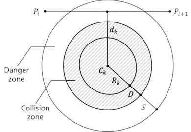
To prevent UAV - obstacle collisions, paths must avoid threat areas modeled as cylinders, with their projections represented by the center and radius .
Threat Cost Function: For the path segment vector , the threat cost is determined by the minimum distance to the threat center , as shown in Eq. (3):
where is the safety distance, is the collision zone width which is related with UAV diameter, is the threat radius, and is the minimum distance between the path segment and the threat center. To minimize the influence of noise in minimum distance calculations, such as those introduced by discrete sampling or terrain artifacts, such as a safety buffer is incorporated in the cost function. Furthermore, the elevation data is preprocessed by smoothing or interpolation to suppress local discontinuities and ensure stability in path evaluation.
The total threat cost is given by Eq. (4):
where is the total number of threats.
Fig. 1Determination of the threat cost
2.1.3. Flight altitude constraints
The UAV’s flight altitude must be maintained within a permissible range, between and . Consequently, a flight altitude cost function is defined.
For the path point , the altitude cost is calculated as Eq. (5):
where is the height of path point , and are the minimum and maximum allowable flight heights, respectively. The total altitude cost is given by Eq. (6):
2.1.4. Smoothness constraints
Path smoothness, determined by turning angles and climb angles, better matches UAV dynamic characteristics. In this study, both turning angle limit and climb angle limit are set to 45°, which is a conservative estimate derived from typical dynamic constraints of fixed-wing and rotary-wing UAV platforms. These values are selected to ensure that generated paths are dynamically feasible and compliant with UAV maneuvering limits, including constraints on roll rate, pitch angle, and climb performance. Fixed-wing UAVs operating at medium airspeeds often have turning constraints ranging between 30° and 60°, and practical climb angles usually fall within the 20°-45° range, depending on power-to-weight ratio and airframe configuration [19]-[22].
The smoothness cost function is then computed as Eq. (7):
where is the turning angle between path segments and , is calculated via the ground projection of the path segments and the angle between them. The climbing angle is the angle between a path segment and the horizontal plane. and are the climb angles for path segments and , which are determined by the height difference and ground projection length of the path segments. and represent the maximum allowable turning and climb angles, respectively.
2.1.5. Overall cost function
By considering the optimality, safety and feasibility constraints associated with a path , the overall cost function is defined as Eq. (8):
where is the weight for each cost component. to represents the path length (2), threat (4), altitude constraint (6), and smoothness (7). By defining these aspects, this paper formulates the UAV path-planning issue as a multi-objective optimization problem. The comprehensive cost function not only reflects path optimality but also incorporates UAV dynamic characteristics and operational constraints, thus generating safe, smooth, and efficient 3D flight paths. The key elements in scene modeling in this study include terrain digital elevation models, cylindrical obstacle parameters, task node coordinates and requirements, and four quantitative constraints.
2.2. Construction of UAV 3D environmental model
To verify the optimization performance of the Starfish Optimization Algorithm in a 3D environment, this study uses MATLAB 2019b to simulate a 3D environment, with the ground information of the simulated mountainous map generated through the following steps.
2.2.1. Terrain construction
In this study, the 3D terrain construction process is implemented using the MATLAB programming language. MATLAB is used for its powerful matrix processing and visualization capabilities, which are well-suited for modeling 3D terrain and simulating UAV flight paths. Specifically, the code first reads elevation data from a Terrain.tif file and converts it into a 2D matrix , where each element represents the height at the corresponding terrain location. To ensure the validity of the elevation data, the code further processes negative values by setting all heights below zero to zero. The size of the elevation matrix also determines the map resolution and horizontal dimensions, which are used to construct a mesh grid via the meshgrid function. This grid enables the 3D terrain surface to be plotted and evaluated as part of the UAV path planning environment.
Then, the code uses the meshgrid function to generate 2D coordinate grids, the meshgrid function generates 2D coordinate matrices from vectors, which are necessary for mapping elevation data over a spatial grid and creating surface plots in 3D. resulting in matrices and , which represent the horizontal and vertical coordinates of the terrain data, respectively. By mapping the height values to each point in the terrain through processing and , a complete 3D terrain model is formed, as shown in Eq. (9):
indicates the terrain height, defining the elevation at each point in a 2D plane. This function outlines the 3D terrain’s basic structure, with terrain height determined by the coordinates, which are used to depict the terrain's undulations.
2.2.2. Threat region construction
Threat regions are modeled as multiple cylinders, each represented by the mathematical function in Eq. (10):
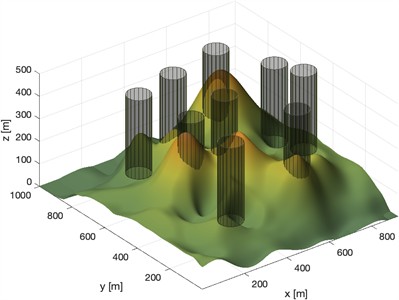
where are the coordinates of the cylinder’s base center, is the cylinder’s radius (indicating the horizontal threat range), and is the cylinder's height (indicating the vertical threat range).
The function uses analytical geometry to define a cylinder’s boundary, defining its position and extent in 3D space. By checking whether a point satisfies the inequality in Eq. (10), the function identifies whether the point lies within the threat region, thus facilitating collision cost computation. Multiple overlapping cylinders create a complex threat environment.
The 3D map generated by MATLAB is shown in Fig. 2.
Fig. 23D UAV environmental model
3. Starfish optimization algorithm
With the rapid development of meta-heuristic algorithms in optimization, bio-inspired algorithms have shown significant superiority in solving multi-dimensional and complex problems. Among these, the Starfish Optimization Algorithm (SFOA) is an emerging bio-inspired meta-heuristic algorithm that simulates the behavior of starfish in nature to provide an innovative solution for global optimization problems.
The SFOA draws inspiration from the behavioral characteristics of starfish and consists of two main phases: exploration and exploitation. In the exploration phase, it mimics the searching ability of starfish arms, using a hybrid five-dimensional and one-dimensional search pattern to enhance search efficiency. In the exploitation phase, it achieves global convergence through predation and regeneration mechanisms.
In the exploration phase, the SFOA employs a hybrid search strategy based on the problem dimension. When the dimension of the optimization problem is greater than 5, the algorithm uses a five-dimensional search pattern to balance the breadth and depth of the search space. When is less than or equal to 5, it adopts a one-dimensional search pattern to improve accuracy. This dynamic adjustment mechanism enables the SFOA to demonstrate remarkable computational efficiency and search ability when dealing with high-dimensional nonlinear optimization problems.
(1) The mathematical model for the exploration phase ( > 5) is as follows, as shown in Eq. (11):
where is the new position of individual in dimension , is the current position of individual in dimension , is the value of the global optimum in dimension for the current population, is the perturbation factor, defined as , used to generate random perturbations, is the angle factor, defined as , used to dynamically adjust the angle, is the current iteration count, and is the maximum number of iterations.
(2) The mathematical model for the exploration phase ( ≤ 5) is as follows, as shown in Eq. (12):
where is the new position of individual in dimension , is the current position of individual in dimension , is the dynamic attenuation factor, defined as , is the position in dimension of the first randomly selected individual in the population, is the position in dimension of the second randomly selected individual in the population, and , are random perturbation factors in the range [–1, 1].
In the exploitation phase, the SFOA uses a bidirectional parallel search strategy and regeneration mechanism to simulate starfish predation and regeneration. The predation phase drives the approach to the global optimum through information sharing among solutions, while the regeneration mechanism enhances the algorithm's global convergence, preventing it from falling into a local optimum. The mathematical model of the predation behavior is shown in Eq. (13):
where is the new position of individual (in vector form, including all dimensions), is the current position of individual (in vector form, including all dimensions), is the global optimum of the current population (in vector form, including all dimensions), is the position of the first randomly selected individual, is the position of the second randomly selected individual, and , are random weight factors in the range [0, 1].
The mathematical model of the regeneration behavior is shown in Eq. (14):
where is current iteration count, is number of individuals in the population, is maximum number of iterations, and is position of the current individual (i.e., the current solution).
The exploitation phase is a highlight of the SFOA. It simulates starfish predation and regeneration. The predation mechanism guides individuals to the global optimum via information sharing, speeding up convergence. Regeneration introduces new diversity to prevent local optima and premature convergence. This bio-inspired strategy revitalizes the population for collaborative optimization. The bidirectional exploitation strategy balances global and local search, giving SFOA strong convergence in complex problems.
Then comes the algorithm update phase. Here, each individual starfish's position is boundary-constrained to stay within the search space. New fitness is calculated and compared to the original. If better, the position and fitness are updated. If the individual's fitness surpasses the current global optimum, the global optimum and its position are updated. This iterative process gradually approaches the optimal solution.
In summary, Hybrid exploration combines high-dimensional and one-dimensional search strategies to balance global and local search efficiency. Adaptive regeneration mimics the starfish’s arm regeneration, reintroducing diversity into the population and avoiding premature convergence. The flowchart of the Starfish Optimization Algorithm is shown in Fig. 3.
Fig. 3Flowchart of the starfish optimization algorithm
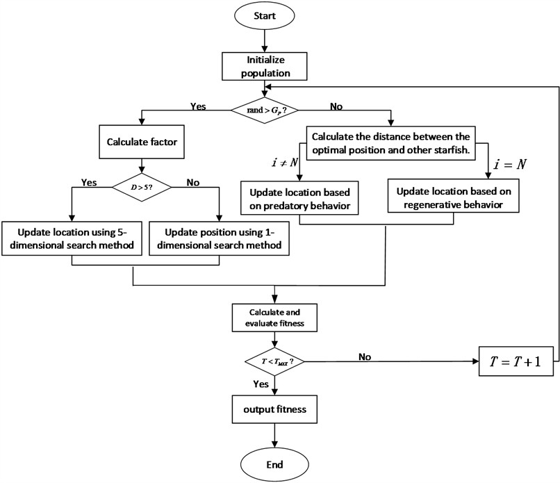
To provide a clearer understanding of the algorithm's operational logic, the flowchart in Fig. 3 illustrates the complete iterative process of the SFOA. The algorithm begins by initializing a population of candidate solutions and evaluating their fitness based on the multi-objective cost function. At each iteration, a decision is made to perform exploration or exploitation based on a dynamic balance factor (GP). In the exploration phase, either a five-dimensional or one-dimensional search pattern is selected depending on the number of problem dimensions, enhancing adaptability and computational efficiency. When in the exploitation phase, the algorithm mimics starfish behaviors such as predation and regeneration to refine the search around promising regions. Throughout the process, individual positions and fitness values are updated, and the global best solution is tracked. After convergence, the optimal trajectory is obtained. In terms of computational complexity, the primary factors influencing performance are the population size, the number of iterations, and the number of decision variables. Each iteration involves operations for fitness evaluation and position updates. Consequently, the overall time complexity of the algorithm is, which is manageable for moderate-scale problems but may require optimization techniques such as parallelization in large-scale or real-time applications.
To cope with large-scale scenarios, SFOA can be parallelized through a two-level strategy: (i) individual-level parallelism maps the fitness evaluation of all Npop starfish to GPU threads within a single CUDA kernel, eliminating the Npop factor from the critical path; (ii) data-level parallelism partitions the high-resolution DEM into tiles, each processed by an independent MPI process, with intra-process OpenMP further accelerating per-tile calculations.
The pseudocode for the Starfish Optimization Algorithm is shown in Table 1.
Table 1The pseudocode for the starfish optimization algorithm
Algorithm 1 SFOA Pseudo-code |
Input: , , , , , Output: , , Curve 01: Set population size and maximum iterations 02: Initialize population and calculate fitness for each individual 03: While 04: Update parameters , theta, based on 05: If rand < % Exploration phase 06: Update positions for each search agent based on high or low dimension strategy 07: Else % Development phase 08: Update positions based on regeneration behavior for last agent 09: End If 10: Calculate fitness for each agent and update best solution 11: Update convergence curve (Curve) 12: 13: End While |
From a mathematical modeling perspective, the SFOA simulates the flexibility of starfish through random factors and multi-dimensional search patterns in its exploration behavior. The predation and regeneration mechanisms dynamically adjust individual positions during iterations, promoting the approach to the global optimum based on the distribution of current solutions. This mathematical framework enables the SFOA to adaptively optimize paths, offering a solid theoretical foundation for multi-objective optimization problems.
These SFOA designs deliver outstanding optimization performance in benchmark tests and real-world engineering problems. Literature verification shows that compared with 100 meta-heuristic algorithms, the SFOA surpasses 95 % in accuracy and 97 % in efficiency, especially in high-dimensional optimization problems.
This paper’s experimental results further confirm the SFOA’s excellent performance in complex optimization problems. Compared with traditional algorithms (Particle Swarm Optimization and Ant Colony Algorithm), the SFOA offers higher computational efficiency, stronger global search ability, and better performance in path smoothness and threat avoidance. This makes the SFOA ideal for high-dimensional, multi-constraint optimization problems like UAV 3D path planning, logistics optimization, and resource allocation.
4. Starfish optimization algorithm for UAV path simulation
This chapter will conduct simulation modeling in MATLAB, with the model involving four key elements. The digital elevation model (DEM) provides terrain elevation data to determine feasible flight altitudes; cylindrical obstacles restrict accessible airspace and introduce safety constraints; mission nodes represent spatial targets with mission requirements; and four quantitative constraints – path length, safety distance, altitude range, and smoothness collectively evaluate the feasibility and quality of the planned drone trajectory.
4.1. Simulation settings
To verify the SFOA’s capability in UAV path planning, this study conducts simulations with detailed designs of the algorithm's key parameters and path-planning constraints, as shown in Table 2. The parameter settings used in this study, such as population size, GP, and exploration angle, were determined based on preliminary experiments and established references.
Table 2Algorithm parameter settings
Category | Parameter |
Population size | 50 |
Initial balance factor between global and local search (GP) | 0.5, Parameter to control the exploration and exploitation behavior of the algorithm |
Number of path nodes (n) | 15 (excluding the starting and ending points) |
Optimization dimension (nD) | 45 (×3) |
UAV diameter () | 1 m |
In experiment, the start and end points are set as | Start = (260, 50, 150), End = (450, 850, 150) |
Flight altitude constraints of the UAV | The UAV’s flight altitude is restricted to between 100 m and 200 m above the terrain surface |
Maximum turning angle | 45° |
Maximum climb angle | 45° |
Safety distance | 10 m |
Nine threat regions (cylinders) are arranged in the terrain, with parameters including center coordinates, height, and radius. For specifics on all obstacles, refer to Table 3.
Table 3Coordinates, radius and heights of all obstacles
Obstacle ID | Center points coordinates | Radius | Heights |
1 | 250, 150, 150 | 50 | 350 |
2 | 200, 650, 150 | 50 | 350 |
3 | 300, 460, 100 | 50 | 350 |
4 | 400, 700, 150 | 50 | 350 |
5 | 450, 450, 150 | 50 | 350 |
6 | 600, 200, 150 | 50 | 350 |
7 | 640, 750, 150 | 50 | 350 |
8 | 800, 600, 100 | 50 | 350 |
9 | 800, 420, 150 | 50 | 350 |
The UAV path objective function consists of four parts: path length cost , threat cost , flight altitude cost , and smoothness cost . The total cost is their weighted sum, calculated by Eq. (15). The optimal solution is defined as the minimum comprehensive cost across all candidate trajectories evaluated during the iterative process. SFOA updates the global best position whenever a better solution is found, and the final reported optimal cost corresponds to the lowest cost obtained at convergence:
In this paper’s simulation, the weight coefficients are set as follows: 0.2, 0.4, 0.2, 0.2.
4.2. Comparison and analysis of simulation results
To assess the effectiveness and scalability of the SFOA-based drone path planning method, we conducted two simulation experiments under different levels of environmental complexity. The first experiment was designed in a relatively simple scenario with five static obstacles, while the second experiment involved a more complex environment with nine obstacles. In both experiments, we compared the performance of SFOA with two widely used meta-heuristic algorithms: ant colony optimization (ACO) and particle swarm optimization (PSO). The experiments collected data at 100 iterations, 500 iterations, and 1,000 iterations to assess the baseline performance and scalability of the algorithms as problem complexity and the number of iterations increased.
4.2.1. Experiments in a simple environment
In this scenario, the drone is tasked with navigating a 3D environment containing five cylindrical threat zones. Environmental parameters are shown in Table 3, and SFOA parameter settings are shown in Table 2. The population sizes for ACO and PSO are the same as those for SFOA. These three algorithms were executed with 100, 500, and 1000 iterations, respectively. For each case, we simultaneously present the optimized 3D flight trajectories, as shown in Fig. 4. The corresponding convergence curves are shown in Fig. 5.
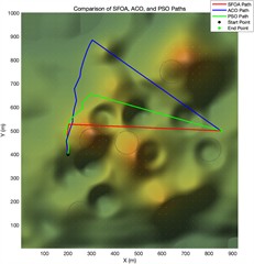
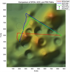
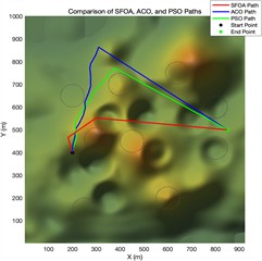
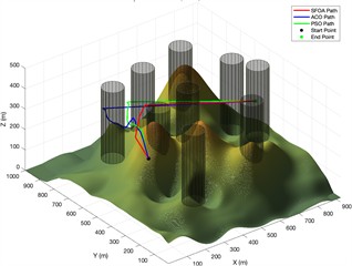
Fig. 4Trajectory planning diagram in a simple experimental environment

a) Top view of flight path planning after 100 iterations of different algorithms

b) Side view of flight path planning after 100 iterations of different algorithms
c) Top view of flight path planning after 500 iterations of different algorithms
d) Side view of flight path planning after 500 iterations of different algorithms

e) Top view of flight path planning after 1000 iterations of different algorithms
f) Side view of flight path planning after 1000 iterations of different algorithms
The convergence curve is shown in Fig. 5.
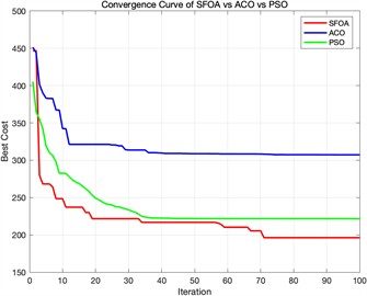
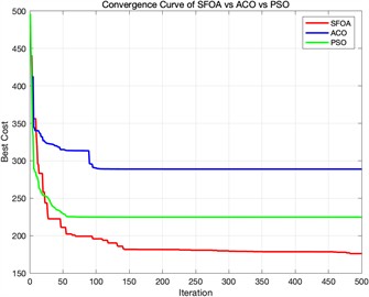
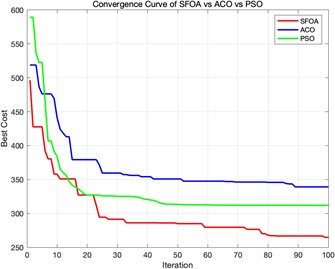
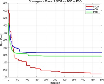
Fig. 5Algorithm fitness convergence curve diagram
a) Fitness convergence curve diagram when different algorithms are iterated 100 times
b) Fitness convergence curve diagram when different algorithms are iterated 500 times
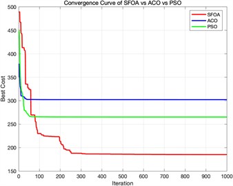
c) Fitness convergence curve diagram when different algorithms are iterated 1000 times
Algorithm fitness convergence curve diagram Fig. 4 shows the 3D path planning results and convergence curves of ACO, PSO, and SFOA under three different iteration settings. The subplots on the far left of each row display the top-down trajectories on the terrain, while the subplots on the right show the corresponding 3D flight paths between obstacles. In all cases, SFOA paths consistently achieve shorter and smoother routes, more efficiently avoiding obstacles while maintaining a balanced altitude distribution. Especially at low iteration counts, SFOA can find competitive paths as early as 100 iterations, while ACO and PSO produce longer and less optimized trajectories. This indicates that SFOA exhibits superior convergence performance in the early stages
The convergence plot in Fig. 5 further supports this observation. At 100 iterations, SFOA exhibits the fastest trend of decreasing total cost, significantly outperforming ACO and PSO. At 500 and 1000 iterations, SFOA continues to improve steadily and reaches the lowest final cost, while ACO stagnates early on and PSO converges at a slower rate. As the number of iterations increases, the gap between SFOA and the other two algorithms widens further, highlighting SFOA's robustness and scalability.
Specific experimental data are shown in Table 4.
Table 4Comparison of simulation results
Iteration | Algorithm | Time taken (s) | Average | Standard deviation | Optimal value |
100 | SFOA | 0.69 | 220.0087 | 37.4293 | 196.1974 |
ACO | 0.74 | 319.4148 | 26.7407 | 307.3099 | |
PSO | 0.71 | 238.7353 | 34.7276 | 221.4830 | |
500 | SFOA | 3.58 | 191.6742 | 34.6347 | 171.6709 |
ACO | 3.94 | 295.6567 | 18.1126 | 315.2578 | |
PSO | 3.99 | 228.8928 | 20.5604 | 292.1947 | |
1000 | SFOA | 6.18 | 204.9176 | 51.0014 | 185.1284 |
ACO | 6.87 | 302.8948 | 4.7793 | 302.2744 | |
PSO | 6.73 | 267.3955 | 14.6430 | 265.1127 |
Table 4 summarizes the best cost achieved by SFOA, ACO, and PSO in the simple environment with five obstacles. SFOA significantly outperforms both comparison algorithms. At 100 iterations, SFOA reduces costs by 36.15 % compared to ACO and 11.42 % compared to PSO. With increased iterations, the performance advantage remains stable or improves – at 500 iterations, the improvement reaches 45.52 % (vs ACO) and 41.24 % (vs PSO). These results demonstrate SFOA’s superior search efficiency and optimization accuracy even in relatively simple terrain configurations.
Overall, trajectory visualization and convergence behavior indicate that SFOA can quickly and reliably generate high-quality paths in simple environments, making it a powerful optimization algorithm for real-time or time-constrained drone missions.
4.2.2. Experiment in a complex environment
To further evaluate scalability, we conducted a second experiment in a more complex scenario with higher obstacle density, which included nine obstacles and increased spatial constraints and solution search space. The test settings used in the experiment are shown in Tables 2 and 3. For each case, we present the optimized 3D flight trajectories, as shown in Fig. 6. The corresponding convergence curves are shown in Fig. 7.
The convergence curve is shown in Fig. 7.
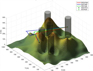
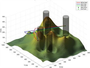
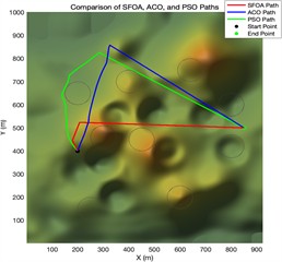
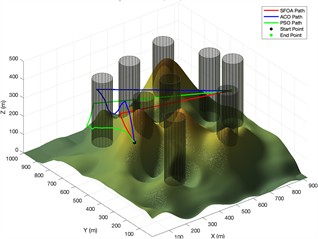
Fig. 6Trajectory planning diagram in a Complex experimental environment
a) Top view of flight path planning after 100 iterations of different algorithms
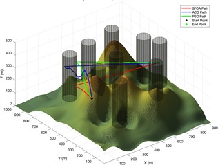
b) Side view of flight path planning after 100 iterations of different algorithms
c) Top view of flight path planning after 500 iterations of different algorithms
d) Side view of flight path planning after 500 iterations of different algorithms
e) Top view of flight path planning after 1000 iterations of different algorithms
f) Side view of flight path planning after 1000 iterations of different algorithms
Fig. 7Algorithm fitness convergence curve diagram
a) Fitness convergence curve diagram when different algorithms are iterated 100 times
b) Fitness convergence curve diagram when different algorithms are iterated 500 times
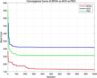
c) Fitness convergence curve diagram when different algorithms are iterated 1000 times
Fig. 6 shows the simulation results in a more challenging 3D terrain containing nine cylindrical obstacles. The results show three iteration settings for the ACO, PSO, and proposed SFOA algorithms. Like the previous section, each row shows the top-view paths, 3D flights trajectories, and convergence curves for the three algorithms.
As can be seen from the figure, the superiority of SFOA becomes even more evident under these more constrained conditions. Even in complex environments, the SFOA trajectory adopts shorter, smoother, and more obstacle-avoidant paths across all iteration settings.
In the convergence curve plot, the SFOA curve rapidly decreases and converges to a lower final cost than the other two algorithms, and this holds true at all iteration levels. The red curve also exhibits lower volatility, indicating better stability and fewer local minimum traps. Additionally, a visual comparison of 3D paths shows that SFOA navigates more effectively in narrow spaces between obstacles. This supports the conclusion that SFOA has stronger global search and constraint handling capabilities, especially as environmental complexity increases.
Specific experimental data are shown in Table 4.
Table 5Comparison of simulation results
Iteration | Algorithm | Time taken (s) | Average | Standard deviation | Optimal value |
100 | SFOA | 0.89 | 299.5491 | 43.9956 | 264.7615 |
ACO | 0.98 | 367.8600 | 43.5554 | 339.1565 | |
PSO | 1.01 | 335.1795 | 55.7187 | 312.0123 | |
500 | SFOA | 4.43 | 214.0971 | 66.4972 | 171.6709 |
ACO | 5.11 | 323.1564 | 26.7845 | 315.2578 | |
PSO | 4.97 | 299.9072 | 21.4181 | 292.1947 | |
1000 | SFOA | 8.52 | 173.0144 | 14.0124 | 164.3933 |
ACO | 9.86 | 312.5457 | 16.2351 | 309.1856 | |
PSO | 9.90 | 259.6608 | 17.3646 | 256.1049 |
The quantitative comparison in Table 5 highlights the performance advantage of SFOA over ACO and PSO in the complex environment. At 100 iterations, SFOA reduces the best cost by 21.91 % and 15.12 % compared to ACO and PSO, respectively. With more iterations, the advantage becomes more pronounced – at 1000 iterations, SFOA outperforms ACO and PSO by 46.84 % and 35.81 %, respectively. These results affirm the algorithm’s superior global search capability and convergence performance, particularly in high-dimensional, obstacle-dense environments.
The two simulation experiments conducted in this study comprehensively evaluated the performance of the SFOA-based path planning algorithm in environments of varying complexity. In a simple scenario with five obstacles, SFOA demonstrated faster convergence speed and better path quality even with a limited number of iterations. Compared to ACO and PSO, SFOA consistently generates shorter, smoother trajectories with lower cost values and better obstacle avoidance performance. In a complex environment involving nine obstacles, the advantages of SFOA become even more pronounced. As the number of dimensions and obstacle density increase, the algorithm maintains robust performance. It demonstrates strong global search capabilities and is less prone to premature convergence. Convergence curves further confirm its efficiency and stability at different iteration levels.
In both cases, SFOA achieves the lowest optimal cost, smallest standard deviation, and fastest convergence speed in most test settings, not only demonstrating its effectiveness but also consistency. Additionally, its performance scales well with increasing problem complexity and iteration counts, supporting its application in constrained and large-scale drone mission planning. These results validate the effectiveness, robustness, and scalability of the SFOA algorithm in multi-objective 3D drone trajectory planning tasks, making it a competitive choice for real-world deployment.
5. Conclusions
This study proposes and validates a three-dimensional UAV path-planning method based on the Starfish Optimization Algorithm tailored for complex environments. A comprehensive cost function is formulated, integrating multiple constraints, such as path length, flight altitude, obstacle avoidance, and path smoothness to address the multi-objective nature of the problem. A detailed 3D environmental model is constructed, incorporating terrain undulations and threat regions, and multiple optimization objectives are designed accordingly.
Experimental results demonstrate that SFOA exhibits strong global and local optimization capabilities, enabling it to efficiently generate safe, smooth, and optimal flight paths in complex 3D environments. Compared to Ant Colony Optimization and Particle Swarm Optimization, SFOA achieves superior performance in terms of path smoothness, convergence speed, and overall cost. During the optimization process, it effectively avoids obstacles, shortens flight time, and reduces energy consumption, thereby validating its effectiveness in multi-objective path planning.
Despite its promising performance, the current implementation of SFOA has certain limitations. The high iteration count, and computational complexity of the cost function limit its applicability in real-time scenarios. Moreover, the algorithm relies on manually tuned parameters, which may require adjustment for different operational environments, reducing its adaptability. Additionally, the current model assumes static threat configurations; its performance may degrade in dynamic environments involving moving obstacles.
Future research will focus on improving the real-time responsiveness, robustness, and scalability of SFOA. Key directions include integrating adaptive parameter tuning mechanisms, employing parallel computing for real-time execution, extending the model to handle dynamic environmental changes, and exploring its applicability in multi-UAV coordination and real-time path adjustment in dynamic mission contexts.
References
-
Y. Yang, Y. Fu, D. Lu, H. Xiang, and K. Xu, “Three-dimensional unmanned aerial vehicle trajectory planning based on the improved whale optimization algorithm,” Symmetry, Vol. 16, No. 12, p. 1561, Nov. 2024, https://doi.org/10.3390/sym16121561
-
Y. Song, X.-L. Ding, and C. Cheng, “UAV path planning based on improved ant colony algorithm,” Manufacturing Automation, Vol. 46, No. 12, pp. 61–67, Dec. 2024, https://doi.org/10.3969/j.issn.1009-0134.2024.12.009
-
G. Nannicini, D. Delling, D. Schultes, and L. Liberti, “BidirectionalA* search on time‐dependent road networks,” Networks, Vol. 59, No. 2, pp. 240–251, May 2011, https://doi.org/10.1002/net.20438
-
R. A. Conn and M. Kam, “On the moving-obstacle path-planning algorithm of Shih, Lee, and Gruver,” IEEE Transactions on Systems, Man, and Cybernetics, Part B (Cybernetics), Vol. 27, No. 1, pp. 136–138, Feb. 1997, https://doi.org/10.1109/3477.552194
-
M. G. Park, J. H. Jeon, and M. C. Lee, “Obstacle avoidance for mobile robots using artificial potential field approach with simulated annealing,” in IEEE International Symposium on Industrial Electronics Proceedings, Vol. 3, pp. 1530–1535, Nov. 2025, https://doi.org/10.1109/isie.2001.931933
-
F. Aurenhammer, “Voronoi diagrams-a survey of a fundamental geometric data structure,” ACM Computing Surveys, Vol. 23, No. 3, pp. 345–405, Sep. 1991, https://doi.org/10.1145/116873.116880
-
Y. Chen, J. Yu, Y. Mei, S. Zhang, X. Ai, and Z. Jia, “Trajectory optimization of multiple quad-rotor UAVs in collaborative assembling task,” Chinese Journal of Aeronautics, Vol. 29, No. 1, pp. 184–201, Feb. 2016, https://doi.org/10.1016/j.cja.2015.12.008
-
D. Karaboga and B. Basturk, “A powerful and efficient algorithm for numerical function optimization: artificial bee colony (ABC) algorithm,” Journal of Global Optimization, Vol. 39, No. 3, pp. 459–471, Oct. 2007, https://doi.org/10.1007/s10898-007-9149-x
-
C. Mou, W. Qing-Xian, and J. Chang-Sheng, “A modified ant optimization algorithm for path planning of UCAV,” Applied Soft Computing, Vol. 8, No. 4, pp. 1712–1718, Sep. 2008, https://doi.org/10.1016/j.asoc.2007.10.011
-
Y. Liu, X. Zhang, Y. Zhang, and X. Guan, “Collision free 4D path planning for multiple UAVs based on spatial refined voting mechanism and PSO approach,” Chinese Journal of Aeronautics, Vol. 32, No. 6, pp. 1504–1519, Jun. 2019, https://doi.org/10.1016/j.cja.2019.03.026
-
Y. Hao, W. Zu, and Y. Zhao, “Real-time obstacle avoidance method based on polar coordination particle swarm optimization in dynamic environment,” in 2nd IEEE Conference on Industrial Electronics and Applications, pp. 1612–1617, May 2007, https://doi.org/10.1109/iciea.2007.4318681
-
C. Zhang, Z. Zhen, D. Wang, and M. Li, “UAV path planning method based on ant colony optimization,” in Chinese Control and Decision Conference (CCDC), pp. 3790–3792, May 2010, https://doi.org/10.1109/ccdc.2010.5498477
-
Z. Xu, “Rotary unmanned aerial vehicles path planning in rough terrain based on multi-objective particle swarm optimization,” Journal of Systems Engineering and Electronics, Vol. 31, No. 1, pp. 130–141, Jan. 2020, https://doi.org/10.21629/jsee.2020.01.14
-
Z. Xu, Y. Wang, and Q. Xiong, “Research on photomask defects path optimization based on ant colony algorithm mixed with 2-opt,” Optoelectronic Technology, Vol. 41, No. 4, pp. 274–279, 2021.
-
J. Zhan, C. Niu, and X. Wan, “Grey wolf optimization algorithm based on optimal individual information fusion strategy,” Journal of Information Engineering University, Vol. 25, No. 6, pp. 710–716, Dec. 2024.
-
C. Zhong, G. Li, Z. Meng, H. Li, A. R. Yildiz, and S. Mirjalili, “Starfish optimization algorithm (SFOA): a bio-inspired metaheuristic algorithm for global optimization compared with 100 optimizers,” Neural Computing and Applications, Vol. 37, No. 5, pp. 3641–3683, Dec. 2024, https://doi.org/10.1007/s00521-024-10694-1
-
M. D. Phung and Q. P. Ha, “Safety-enhanced UAV path planning with spherical vector-based particle swarm optimization,” Applied Soft Computing, Vol. 107, p. 107376, Aug. 2021, https://doi.org/10.1016/j.asoc.2021.107376
-
Y. Yang, Y. Fu, R. Xin, W. Feng, and K. Xu, “Multi-UAV trajectory planning based on a two-layer algorithm under four-dimensional constraints,” Drones, Vol. 9, No. 7, p. 471, Jul. 2025, https://doi.org/10.3390/drones9070471
-
J. Akshya et al., “Geometric optimisation of unmanned aerial vehicle trajectories in uncertain environments,” Vehicular Communications, Vol. 54, p. 100938, Aug. 2025, https://doi.org/10.1016/j.vehcom.2025.100938
-
R. Li, G. Chen, Y. Lu, K. Qin, T. Zhou, and W. Wang, “Longitudinal perching trajectory planning for a fixed-wing unmanned aerial vehicle at high angle of attack based on the estimation of region of attraction,” Drones, Vol. 9, No. 2, p. 87, Jan. 2025, https://doi.org/10.3390/drones9020087
-
T. Zhang, J. Yu, J. Li, and J. Wei, “Upgraded trajectory planning method deployed in autonomous exploration for unmanned aerial vehicle,” International Journal of Advanced Robotic Systems, Vol. 19, No. 4, Jul. 2022, https://doi.org/10.1177/17298806221109697
-
S. Lee, H. Kang, J. Lee, and Y. Kim, “Optimal policy of pitch-hold phase for mine detection of UAV based on mixed-integer linear programming,” International Journal of Aeronautical and Space Sciences, Vol. 23, No. 4, pp. 746–754, Mar. 2022, https://doi.org/10.1007/s42405-022-00454-7
About this article

This study has been supported by the Open Fund Project of Key Laboratory of Civil Aviation Flight Technology and Fight Safety (Grant No. FZ2021ZZ06). This work has also been supported by Central University Basic Research Projects (Grant No. 24CAFUC04002) and the Sichuan Engineering Research Center for Smart Operation and Maintenance of Civil Aviation Airports (Grant No. JCZX2023ZZ07 and No. JCZX2024ZZ25). This work has also been supported by Sichuan Flight Engineering Technology Research Center Project (Grant No. GY2024-30D). This work has also been supported by Student Innovation and Entrepreneurship Training Program (Grant No. 202510624005).
The datasets generated during and/or analyzed during the current study are available from the corresponding author on reasonable request.
Weiqi Feng was responsible for the conceptualization, formal analysis of this research, data curation, writing-original draft preparation. Yujie Fu and Yong Yang were responsible for the research methodology, formal analysis, and visualized the experimental results. Changjian Gao and Kaijun Xu validated the effectiveness of the experimental results and contributed to the manuscript writing.
The authors declare that they have no conflict of interest.
