Abstract
Accurate positioning in space is an important foundation for ensuring the stability of autonomous flight and successful mapping and navigation of unmanned aerial vehicles (UAVs). At present, the SLAM algorithm based on the Cartographer algorithm for real-time positioning and mapping is widely used in fields such as robot navigation and autonomous driving. However, in the context of UAV applications, this algorithm has a high dependence on the amount of point cloud information in the surrounding environment, and cannot achieve precise positioning in open spaces with insufficient lighting and fewer feature points, resulting in significant mapping errors. In order to solve the problem of low positioning estimation accuracy in the Cartographer algorithm in above environment, this paper proposes a precise positioning algorithm for UAVs that integrates VIO and Cartographer. This algorithm can continuously output more accurate position estimation information during UAV flight, compensating for the problem of inaccurate position estimation caused by partial feature loss or coordinate system drift in point clouds. In addition, this algorithm ensures navigation obstacle avoidance in narrow spaces by improving positioning accuracy and mapping accuracy, making it more applicable in the field of UAVs. Finally, the effectiveness of the proposed positioning algorithm was verified through experimental analysis of the Cartographer dataset and practical testing of UAVs in real scenarios.
1. Introduction
The key technology for mobile robots to achieve autonomous movement in unknown environments is known as Simultaneous Localization and Mapping (SLAM) [1]. Accurate positioning in space is an important foundation for ensuring the stability of autonomous flight and successful mapping and navigation of UAVs [2]. At present, the commonly used laser SLAMs for indoor positioning of UAVs include Hector SLAM, Karto SLAM, Gmapping, and Cartographer [3]. The Cartographer algorithm is a set of graph optimized laser SLAM algorithms launched by Google and it has been widely used in intelligent vehicles, robots, UAVs and other fields due to its advantages of high accuracy, good real-time performance and stability [4]. In recent years, many researchers and developers have made improvements to Cartographer, including improving the efficiency and accuracy of map construction, and increasing adaptability to dynamic environments. However, due to the fact that the Cartographer uses unscented Kalman filter to process LiDAR data to obtain the observed position [5], the method of obtaining the observed position based on inertial measurement sensor data and point cloud matcher has issues with position estimation lag and accuracy [6-7]. Hess et al. proposed a real-time loop closure algorithm [8], which updates the position estimation of the robot by utilizing closed-loop constraints in a local map and eliminates the lag in position estimation by combining it with a global map. This algorithm can significantly improve the position estimation accuracy and real-time performance of the Cartographer algorithm. However, in open environments, the point cloud data information provided by radar is insufficient, and the point cloud data information within the scanning radius range constantly changes, making it difficult to form closed-loop constraints, and the position estimation accuracy cannot achieve ideal results. Ye et al. proposed a method for integrating inertial sensor data with LiDAR data [9], which can reduce computational resource requirements and improve positioning accuracy and map construction stability. However, in the application scenario of rapid movement of UAVs, coordinate system drift may occur. [10] Gao et al. [10] proposed VIO (visual-inertial odometry) as the front-end algorithm for SLAM mapping in the application of quadruped robots, and processed the image data of binocular cameras through LK optical flow tracking [11] and pre-integrated IMU data [12], optimizing the close fusion of inertial sensor data and visual data, greatly improving positioning accuracy. However, in the case of rapid movement of UAVs, visual data noise is high, leading to inaccurate positioning of the odometer output by VIO tight coupling and a decrease in positioning accuracy. Huang et al. [13] proposed the wheel based odometry method to eliminate motion distortion, reduce cumulative errors, and improve map construction performance. However, for UAVs, odometry information can only be provided through the IMU of flight control, and the accuracy is not as accurate as the pose obtained through wheels.
To sum up, although there are many improved Cartographer algorithms currently available, most of them have certain limitations in the application direction of drones due to their rich environmental characteristics, complex structures, and static scenes. To solve the problem of insufficient point cloud data and fast moving coordinate system drift in open environments, we propose an algorithm that integrates VIO to optimize Cartographer position estimation based on our previous experience in engineering measurement research on underwater robots and structural vibration [14-15]. In addition to radar data and flight control IMU data, the position data of optimized tightly coupled binocular vision VIO is also introduced into the position estimation of the algorithm. After preprocessing these two kinds of data, the Kalman filter is used to output more accurate position information to the SLAM algorithm. This algorithm can provide initial position information for point cloud matching nonlinear least squares calculation, thereby enhancing the accuracy of mapping. By comparing the experimental data with the original algorithm, the improved algorithm achieves more accurate positioning, smaller coordinate system drift error, stronger robustness, and more accurate map construction.
This paper is organized as follows: Section 2 is the basic theory derivation for algorithm construction. In Section 3, we constructed an improved cartographer algorithm that integrates VIO. Section 4 is devoted to experimental validation of the proposed improved cartographer algorithm integrating VIO using an UAV. Conclusions close the paper in Section 5.
2. Algorithm construction
Cartographer laser SLAM mapping is a type of SLAM synchronous positioning and map construction algorithm. It refers to the robot starting from an unknown location in an unknown environment, positioning its pose through repeatedly observed point cloud features during its movement, and then constructing an incremental map based on its own position, thereby achieving the goal of simultaneous positioning and map construction. The use of Ceres nonlinear optimization method and the idea of constructing a global map based on submap can effectively avoid interference from moving objects in the environment during the mapping process. In each frame, the Cartographer generates a new submap based on the LiDAR data in the current frame and matches it with the submap from the previous frame. If there are overlapping areas between two submaps, the loopback detection function [16] can be used for precise spatial mapping.
2.1. Coordinate transformation
The construction of precise maps using the Cartographer algorithm requires data information from multiple different sensors, which often requires a certain coordinate transformation before being used by the algorithm. Coordinate transformation helps UAVs align multiple data coordinate systems in different environments, achieving precise positioning and map building functions. Taking the inertial odometer, two-dimensional radar, and depth camera as examples in unmanned aerial vehicles, the coordinate relationship in centimeter length units is shown in Fig. 1.
Fig. 1Schematic diagram of sensor coordinate system
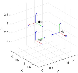
The Cartographer algorithm uses a transformation matrix to achieve coordinate transformation. The algorithm converts the data of each sensor based on the given position and direction of each sensor. Taking the coordinate transformation of radar sensors as an example, its transformation matrix relationship can be represented by Eq. (1):
where is a point in the LiDAR coordinate system, is a point in the map coordinate system, is the translation matrix, and is the rotation matrix. By using this transformation matrix, the coordinate information of various sensors at different spatial positions is integrated into the same coordinate system. After coordinate unification, the algorithm can continuously calculate the robot’s position based on data from multiple sensors, improving the accuracy of position estimation.
2.2. Local SLAM and global SLAM
The Cartographer algorithm can be treated as two relatively independent and interrelated subsystems. The first is the local SLAM (front-end), which is responsible for establishing a series of submaps, outputting and storing odometers and submaps. The second is global SLAM (back-end), which matches the submaps generated by the front-end according to the timestamp, and then optimizes the global submaps and odometers. The Cartographer algorithm first processes the LiDAR data in the front-end stage. The radar provides a frame of point cloud information every time it scans, and is converted into point cloud data in the radar coordinate system according to Eq. (2):
where is the position of the three-dimensional point on the radar coordinate system, is the radian required to rotate around the -axis to return to the radar coordinate system. Matching the converted radar data with the previous submap, the position of the point beam falls to the optimal position on the submap after conversion. As the data frames are continuously inserted, they are combined to form a new submap. Subsequently, in order to eliminate sensor measurement errors and improve the accuracy of the map, was optimized through matching algorithms and outputing the optimal pose for matching. This least squares problem can be solved by using the Ceres library in Cartographer according to Eq. (3):
where is a linear evaluation function, is the position in the submap coordinate system, and is a subset of the square radius of the Submap. Through this optimization method, Cartographer has higher accuracy than raster maps. Therefore, the adjacent two submaps obtained through scan matching during the mapping process are relatively accurate, but there are still cumulative errors compared to the global SLAM. The Cartographer algorithm adopts a branch and bound optimization method for optimization search, which can efficiently search for the best match in the global position space. For candidate positions, only one matching score needs to be calculated, and the pre-calculated values can be used to accelerate this calculation, thereby improving search efficiency and improving the accuracy of mapping.
2.3. Visual inertia odometer (VIO) algorithm
At present, the main navigation systems for UAVs include GPS satellite navigation systems, integrated navigation systems with LIDAR and inertial navigation. However, when the GPS signal is weak or there is significant environmental interference during the navigation process, the effectiveness of the data of these navigation systems is greatly reduced. The VIO algorithm for tightly coupled binocular camera IMU data and visual data can effectively solve the above problems. By aligning the IMU pose sequence with the camera pose sequence, the true scale of the camera trajectory can be obtained. The VIO-SlAM is divided into three parts in this paper: front-end visual inertial navigation odometer, back-end nonlinear optimization, and loop detection, as shown in Fig. 2.
Fig. 2Schematic diagram of VIO-SLAM structure
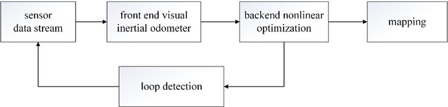
Adopting the binocular LK optical flow method for feature tracking and built-in IMU pre-integration processing to optimize the tightly coupled VIO algorithm theory, the sliding window is optimized for tightly coupled backend nonlinearity, and loop detection and repositioning are used to eliminate accumulated errors and improve positioning accuracy.
2.4. Improved cartographer algorithm integrating VIO
The improved Cartographer algorithm based on VIO proposed in this paper tightly couples the IMU of binocular cameras and the visual data of binocular fish eyes with VIO, and outputs the odom data information after fusion with the flight control IMU and LiDAR multi-sensor. After preprocessing, it is converted into robot_local_position and then used Kalman filtering to denoise the incoming data, followed by normalization processing. Finally, the processed data is input into the Kalman filter for state estimation, and the position estimation value is calculated based on the state estimation results, greatly improving robustness and accuracy of position estimation. Applying the processed position information to the Cartographer algorithm for mapping can improve the accuracy of the map.
2.5. Optimized tightly coupled VIO position output
Using LK optical flow method for feature tracking in VIO tightly coupled binocular fish eye visual data and pre-integrated binocular camera IMU data, the optimized variables are calculated using Jacobian matrix and covariance matrix through minimum edge residual, visual residual, etc. Finally, loop detection is performed to improve the accuracy of the output position information. The LK optical flow method tracks the movement of image pixels, while and represent the position of pixels in the image. By using the least squares method, the position movement of pixels within time can be calculated, as shown in Eq. (4):
The feature quantity to be estimated is the spatial three-dimensional coordinates , and the observed values are the coordinates of the feature points on the camera normalization plane. Therefore, the observed values cannot be directly output as position information. It is necessary to transform the matrix and perform inverse depth parameterization to meet the Gaussian system, and calculate the three-dimensional coordinate output. The equation is shown in Eq. (5):
where is the inverse depth. Then, the optimized visual position data is tightly coupled with the IMU preprocessed pose data for VIO, thereby outputting more stable position information.
2.6. Position output after fusion of LiDAR and flight control IMU
The Cartographer algorithm integrates local SLAM and global SLAM, and both SLAM processes require optimized position information, which is the scanned position data obtained from radar observations . When the radar is applied to UAVs during testing, the platform cannot achieve decisive stability, so it integrates the IMU (Inertial Measurement Unit) of flight control. IMU will provide the direction of gravity, which is used to project radar data onto the 2D plane, provide the radar with an attitude, and determine the 2D plane scanned by the radar. Mapping navigation requires submap matching, and the construction of submap is an iterative process of continuously aligning Scans with the coordinate system of submap. Scans' data is obtained from each frame of the radar using Eq. (6):
where is the radius size of the submap. When matching and aligning the obtained Scans’ data with the submap, it needs to be converted into the position of the radar frame in the submap coordinate system . The conversion can be done through Eq. (7):
Through the transformed position , the constructed submap can be matched to obtain more accurate maps.
2.7. Optimization of position information output using Kalman filtering
The front-end of the Cartographer is responsible for inputting and storing position information data. In order to provide accurate position information for it, this paper constructs a sequence by pruning to ensure that all data timestamps are in order before tightly coupled VIO pose data and LiDAR fusion flight control IMU data fusion. Then, the first and last LiDAR odometer data and VIO odometer data are taken out, and the position transformation relationship at two time points is calculated using Eq. (8):
where is the position transformation from the last data to the first data, and is the first received VIO or Lidar position data. is the VIO or Lidar position data received at the last moment. Calculate the translation from the last data to the first data, and then divide by the elapsed time to obtain the average linear velocity of the , , and axes for that time period. The initial prediction of odom and point cloud position by Cartographer is based on the uniform velocity model, which is often difficult to meet in practical application scenarios. For UAVs, the shorter the running distance, the more capable the uniform velocity model can replace the linear and angular velocities of UAVs. Therefore, using the closest two odometer data for estimation can obtain more accurate odometer data. The position of each timestamp of the UAV can be obtained through an inference device, and its displacement inference mainly relies on the latest line velocity from odom, which is calculated using Eq. (9):
By calculation, Lidar_linearlocal and VIO_linearlocal can be obtained, both of which can be used to calculate and infer the latest speed information and odometer data in UAV coordinate system. However, due to the different accuracy of sensors in different environments, the calculated UAV line speed is weighted and integrated according to Eq. (10) to obtain odometer data:
where robot_local_position is the latest odometer data, and and are the weights of trust for the two postures. The weight of and depends on the variance of Lidar_linearlocal and VIO_linearlocal. Under the conditions of , , and 1, the smaller the data variance, the greater the trust weight.
Obtain the latest odometer information and input it into the Kalman filter for prediction. In Eq. (11), is the current robot_local_position odometer information observation value, is the previous time value, and during the testing process, the UAV is set to move at a constant speed, so the speed remains unchanged:
The simplified matrix equation yields the predicted pose result , where is the hyperparameter, represents the predicted pose from the previous moment, and represents the noise generated during the UAV motion process.
Perform covariance calculation on the predicted pose result from the previous moment, and simplify the equation as shown in Eq. (12):
The covariance of the calculated pose estimation contains the covariance of the prior estimation, remains the covariance of the noise:
where, is the measured value, is the matrix between the observed value and the measured value, is the observed value, and is the noise of the observed value. Apply Eq. (13) to calculate Eq. (14), where is the position measurement value, is the velocity measurement value, is the position observation value, is the velocity observation value, is the observation position noise, and is the observation velocity noise:
In this experiment, only the position is observed without considering the velocity. The observation value is equal to the measurement value, so matrix is [1, 0]. The observation velocity and noise are both 0, and only the pose measurement calculation is considered. Therefore, Eq. (14) can also be simplified into Eq. (15):
The calculated measurement value is in the basic equation (16), and is the predicted value from the previous moment. The accurate pose output is obtained by inputting the corrected estimation result:
The updated Kalman gain Eq. (17) and the updated validation estimation covariance Eq. (18) will yield and , respectively, for the next Kalman filtering process. In Eq. (17), is the variance of the observed noise, which is not considered in this experiment. The value of is 0, and is the identity matrix:
The real-time processing of updated position information through Kalman filtering will make it more accurate, providing it to the local SLAM and global SLAM systems in the Cartographer algorithm to achieve higher positioning accuracy and robustness in mapping.
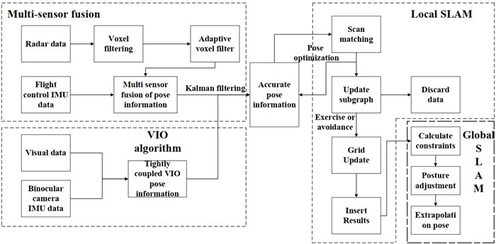
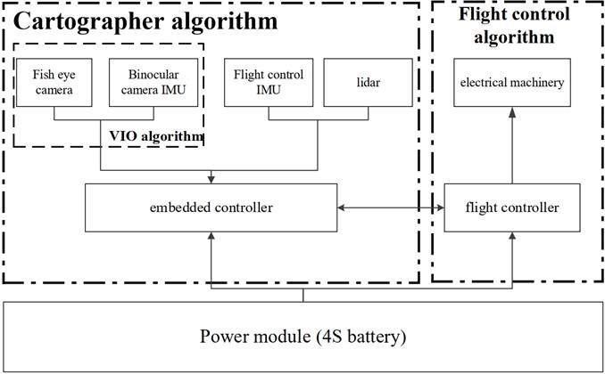
The structure of the improved Cartographer algorithm that integrates binocular VIO is shown in Fig. 3, which is divided into four parts: the VIO algorithm part, the multi-sensor fusion part, the global SLAM, and the local SLAM. Compared to the original Cartographer front-end, the improved algorithm after fusion is responsible for the input, storage, and operation of LiDAR data, and outputs odom data for Cartographer mapping. The improved algorithm solves the problem of inaccurate positioning caused by insufficient point cloud data in complex environments due to map matching using time stamps and the problem of inaccurate positioning accuracy caused by coordinate system drift caused by the rapid movement of the drone when integrating IMU data and LiDAR data for flight control. Combined with the optimized VIO tightly coupled algorithm and Kalman filtering algorithm, it can enhance robustness and adapt to environments with fewer feature points, improve the accuracy of position estimation and ensure the accuracy of the mapping.
Fig. 3Cartographer algorithm framework diagram
3. Experimental validation
After installing the environment dependencies of programs such as the Cartographer algorithm, VIO algorithm, and ROS robot software platform on an embedded platform, the algorithm data input interface was connected to the ROS platform. ROS provides hardware, device drivers, and other functions. In order to facilitate the observation of real-time data, a method of sharing ROS interface data between the host computer and the laptop computer is adopted, and flight instructions are issued and valid data is recorded on the laptop computer.
Fig. 4Photo of the UAV
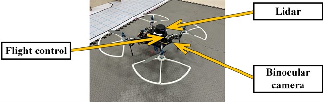
3.1. Design of UAV controller
The hardware platform of this paper is a self-built unmanned aerial vehicle, as shown in Fig. 4. The flight controller is PX4 flight control, using Cortex-M7 core and having a master-slave processor. It can communicate with onboard computers through its own UART serial port or USB interface. The embedded controller is Jetson Orin NX, the binocular camera is RealsenseT265, and the two-dimensional radar is Silan A2M12 LiDAR. The structure and algorithm framework of the entire UAV are shown in Fig. 5.
Fig. 5Hardware structure of quadrotor UAV
3.2. Site layout and experimental testing
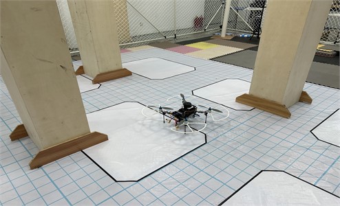
The flight test environment is located inside the safety net site, with three rectangular obstacles placed around the UAV to provide more point cloud information and facilitate the accuracy of the map. The improved algorithm and original algorithm proposed in this paper are tested, and the effectiveness of the algorithm is verified through various data analysis and comparison. The size of the site is within the radar scanning radius, and the takeoff height of the UAV does not exceed the height of the obstacle. The actual test environment is shown in Fig. 6.
Fig. 6Real flight test of UAV in laboratory
4. Comparison and analysis of test data
In order to further verify the accuracy of the improved algorithm, the improved algorithm was run separately from the original algorithm and the VIO algorithm. By using unmanned aerial vehicles for fixed-point flight, the positioning data of 20 sampling points were recorded for two situations: insufficient data in open point clouds and rapid movement. The relative error with the actual position data measured in the environment was calculated and the absolute value was taken, which is shown in Fig. 7 and Fig. 8.
Fig. 7Comparison of absolute relative error values for insufficient point cloud data
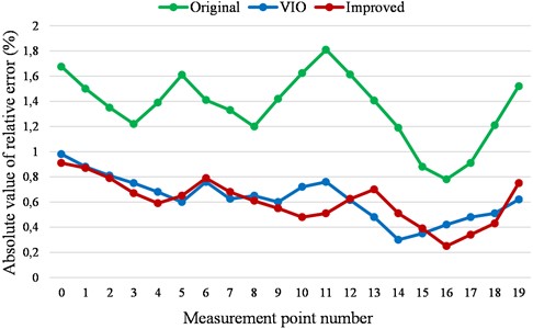
Fig. 8Comparison of absolute values of relative error for rapid movement
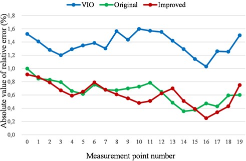
Through the data analysis of Fig. 7 and Fig. 8, it can be concluded that the original algorithm has a large range of absolute relative error changes and obvious curve peaks when the environmental point cloud information is insufficient. The VIO algorithm also has a large fluctuation range of output pose information when moving rapidly. In comparison, the improved algorithm tends to output sensor values with more accurate pose information in either case. Therefore, the improved algorithm that integrates both poses has a smaller relative error in pose information and a smoother and more stable error curve.
Positioning accuracy is one of the important standards for algorithm improvement. In order to evaluate the accuracy of the improved algorithm, local position information data of the integrated UAV is observed and recorded based on the data of these 40 sampling points. Due to the fast refresh rate of data, the average of 10 data records is taken each time, and their absolute translation error, mean square translation error, absolute rotation error, and mean square rotation error are compared item by item. The data records are shown in Fig. 9.
Through analysis of Fig. 9, it can be clearly observed that the improved algorithm has greatly reduced various errors, and the accuracy of positioning is improved by about 19.6 % compared to the original algorithm. In order to further test the actual effectiveness of the algorithm, multiple algorithms and combinations were compared, and the experimental site was mapped as shown in Fig. 10, and more detailed data analysis was conducted.
Fig. 9Data test comparison and quantitative analysis
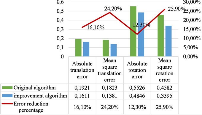
Fig. 102D maps of the laboratory constructed using different algorithms
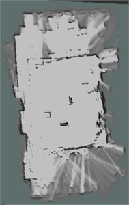
a) Lidar
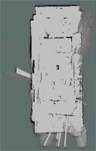
b) Lidar +IMU
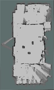
c) Lidar +VIO
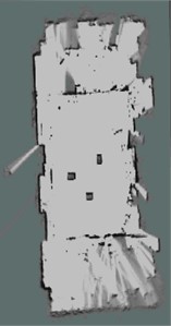
d) Lidar +IMU+VIO
Fig. 10(a) is a map constructed with only LiDAR data, Fig. 10(b) is a map containing LiDAR and IMU data, Fig. 10(c) is a map constructed with LiDAR and VIO data, and Fig. 10(d) is a map constructed with three types of data fusion: LiDAR+IMU+VIO. Fig. 10(a) uses LiDAR as a single source of pose information, resulting in significant map errors. Fig. 10(b) uses IMU data from flight control as auxiliary data, which plays a certain optimization role. Fig. 10(c) shows that the improved algorithm combines VIO data with the original algorithm data from Cartographer for filtering, resulting in significant map optimization. Fig. 10(d) introduces IMU data into the improved algorithm as auxiliary, greatly improving map matching. From the perspective of the constructed maps, it can be seen that the improved algorithm results in a more complete map with almost no coordinate system drift. The combination matching score of each algorithm is shown in Fig. 11.
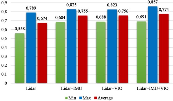
From Fig. 11, it can be intuitively concluded that when VIO is integrated with the Cartographer algorithm for localization, it has the highest matching score. In actual testing, this combination performs better than other combinations in pointing flight. After reaching the designated point, the UAV can perform faster convergence control with higher accuracy, and the accuracy of the map is also increased by about 14.8 %. Based on the test results, it can be further concluded that the improved algorithm not only improves the accuracy of positioning, but also has smaller drift error, achieving the best mapping effect and improving the accuracy of subsequent navigation obstacle avoidance control.
Fig. 11Combination matching score of each algorithm
5. Conclusions
This paper mainly focuses on the problem of inaccurate mapping caused by the inaccurate positioning of the Cartographer algorithm using LiDAR on UAVs. By integrating tightly coupled VIO position information and performing Kalman filter to optimize the position estimation of the Cartographer algorithm, various flight tests and data comparison analysis are conducted to verify the accuracy of the improved algorithm. After comparative analysis, the improved algorithm can stably and continuously output low ripple position information when the UAV is moving rapidly. For some open environments with less point cloud information and environments with fewer spatial feature points due to insufficient lighting, the positioning accuracy of the improved algorithm is improved by about 30 % compared to the original algorithm. The output position information of the improved algorithm is integrated into the Cartographer algorithm, resulting in an increase of about 20 % in map matching and a significant improvement in the accuracy of the flight control system.
References
-
J. J. Leonard and H. F. Durrant-Whyte, “Simultaneous map building and localization for an autonomous mobile robot,” in IROS’91: IEEE/RSJ International Workshop on Intelligent Robots and Systems ’91, Vol. 3, pp. 1442–1447, Feb. 2024, https://doi.org/10.1109/iros.1991.174711
-
H. Durrant-Whyte and T. Bailey, “Simultaneous localization and mapping: part I,” IEEE Robotics and Automation Magazine, Vol. 13, No. 2, pp. 99–110, Jun. 2006, https://doi.org/10.1109/mra.2006.1638022
-
T. Xia and X. Shen, “Research on parameter adjustment method of cartographer algorithm,” in 2022 IEEE 6th Advanced Information Technology, Electronic and Automation Control Conference (IAEAC), pp. 1292–1297, Oct. 2022, https://doi.org/10.1109/iaeac54830.2022.9930054
-
C. Cadena et al., “Past, present, and future of simultaneous localization and mapping: toward the robust-perception age,” IEEE Transactions on Robotics, Vol. 32, No. 6, pp. 1309–1332, Dec. 2016, https://doi.org/10.1109/tro.2016.2624754
-
W. Muhammad and A. Ahsan, “Airship aerodynamic model estimation using unscented Kalman filter,” Journal of Systems Engineering and Electronics, Vol. 31, No. 6, pp. 1318–1329, Dec. 2020, https://doi.org/10.23919/jsee.2020.000102
-
R. Desai, D. Martelli, J. A. Alomar, S. Agrawal, L. Quinn, and L. Bishop, “Validity and reliability of inertial measurement units for gait assessment within a post stroke population,” Topics in Stroke Rehabilitation, pp. 1–9, Aug. 2023, https://doi.org/10.1080/10749357.2023.2240584
-
C. Prados Sesmero, S. Villanueva Lorente, and M. Di Castro, “Graph SLAM built over point clouds matching for robot localization in tunnels,” Sensors, Vol. 21, No. 16, p. 5340, Aug. 2021, https://doi.org/10.3390/s21165340
-
W. Hess, D. Kohler, H. Rapp, and D. Andor, “Real-time loop closure in 2D lidar slam,” in 2016 IEEE International Conference on Robotics and Automation (ICRA), pp. 1271–1278, May 2016, https://doi.org/10.1109/icra.2016.7487258
-
H. Ye, Y. Chen, and M. Liu, “Tightly coupled 3D lidar inertial odometry and mapping,” in 2019 International Conference on Robotics and Automation (ICRA), pp. 3144–3150, May 2019, https://doi.org/10.1109/icra.2019.8793511
-
F. Gao et al., “Positioning of quadruped robot based on tightly coupled LiDAR vision inertial odometer,” Remote Sensing, Vol. 14, No. 12, p. 2945, 2945, https://doi.org/10.3390/rs14122945
-
T. Hu, R. Fuchikami, and T. Ikenaga, “Temporal prediction-based temporal iterative tracking and parallel motion estimation for a 1-ms rotation-robust LK-based tracking system,” IEEE Transactions on Instrumentation and Measurement, Vol. 72, pp. 1–14, Jan. 2023, https://doi.org/10.1109/tim.2023.3295456
-
Y. Huang, G. Wu, and Y. Zuo, “Research on slam improvement method based on cartographer,” in 9th International Symposium on Test Automation and Instrumentation (ISTAI 2022), pp. 349–354, Jan. 2022, https://doi.org/10.1049/icp.2022.3248
-
C. Zhang, L. Chen, and S. Yuan, “ST-VIO: visual inertial odometry combined with image segmentation and tracking,” IEEE Transactions on Instrumentation and Measurement, Vol. 69, No. 10, pp. 1–1, Jan. 2020, https://doi.org/10.1109/tim.2020.2989877
-
X. Du and Q. Fu, “Surrogate model-based multi-objective design optimization of vibration suppression effect of acoustic black holes and damping materials on a rectangular plate,” Applied Acoustics, Vol. 217, p. 109837, Feb. 2024, https://doi.org/10.1016/j.apacoust.2023.109837
-
X. Du, C. Zong, B. Zhang, and M. Shi, “Design, simulation, and experimental study on the hydraulic drive system of an AUV docking device with multi-degree freedom,” Journal of Marine Science and Engineering, Vol. 10, No. 11, p. 1790, Nov. 2022, https://doi.org/10.3390/jmse10111790
-
A. Fișne, M. U. Bahçeci, M. Dursun, S. Aydoğmuș, and Çetintepe, “High-level synthesis based radar hardware implementation and performance comparison,” in 2022 Innovations in Intelligent Systems and Applications Conference (ASYU), pp. 1–6, Sep. 2022, https://doi.org/10.1109/asyu56188.2022.9925373
About this article

This research was funded by the National Key Research and Development Program of China (Grant number 2019YFB2006402), College Students’ Innovative Entrepreneurial Training Plan Program of Jiangsu Province (Grant number 202311276080Y) and the Scientific Research Foundation for High-Level Talents of Nanjing Institute of Technology (Grant number YKJ202102).
The datasets generated during and/or analyzed during the current study are available from the corresponding author on reasonable request.
Conceptualization, Jiaqi Xu and Zhou Chen; Methodology, Jiaqi Xu and Zhou Chen; Software, Jiaqi Xu and Zhou Chen; Validation, Jie Chen and Jingyan Zhou; Formal analysis, Jiaqi Xu and Zhou Chen; Investigation, Zhou Chen; Writing-original draft preparation, Zhou Chen; Writing-review and editing, Xiaofei Du. All authors have read and agreed to the published version of the manuscript.
The authors declare that they have no conflict of interest.
