Abstract
Traditional visual SLAM methods are built on the strong assumption that the system operates in static environments, with limited consideration of moving objects. This assumption often leads to significant performance degradation when dynamic elements are present. To mitigate the impact of moving objects and enhance both localization accuracy and mapping quality, we propose a visual SLAM framework that explicitly removes dynamic object interference from the visual odometry and mapping modules. First, we refine the data association process in visual odometry by introducing motion consistency constraints, which reduce incorrect feature matches and thereby improve pose estimation accuracy. At the same time, depth information from RGB-D sensors is used to validate potentially dynamic feature points. Second, within the mapping module, we formulate keyframe selection as a vertex cover problem to ensure the local representativeness of keyframes. This approach not only reduces mapping artifacts but also enables the comprehensive detection and removal of dynamic objects. Finally, experiments conducted on the TUM RGB-D dataset demonstrate that our system achieves higher accuracy, robustness, and stability compared to baseline methods.

Highlights
- Adopting the GMS algorithm, we filter erroneous matches via motion consistency constraints and verify dynamic points using RGB-D depth information. This dual mechanism overcomes RANSAC’s limitations in dynamic scenes, enhancing pose estimation accuracy and robustness.
- Formulating keyframe selection as a vertex cover problem balances coverage and efficiency. K-D Tree-accelerated DBSCAN (with KNN-adaptive parameters) clusters dynamic points, ensuring thorough removal and high-fidelity static map reconstruction.
- Integrating feature matching, dynamic labeling, and clustering, the framework adapts to low/high-dynamic scenes via initialization-derived parameters. It reduces ATE RMSE by 37.68% (low-dynamic) and 77.57% (high-dynamic) vs. ORB-SLAM2.
1. Introduction
Simultaneous Localization and Mapping (SLAM) [1] is a core perception technology that allows mobile robots to localize themselves while simultaneously constructing maps of their surroundings. Unlike systems that rely on prior environmental knowledge or infrastructure-based positioning technologies (e.g., Bluetooth, WiFi, or Ultra-Wideband anchors), SLAM operates autonomously and estimates real-time poses by integrating data from multiple sensors – commonly cameras, LiDAR, and IMUs – while incrementally generating environmental representations in the form of point clouds or voxel grids.
However, conventional visual SLAM frameworks largely assume static environments, which results in substantial pose estimation errors when applied to dynamic scenes. Quantitative evaluations using the TUM RGB-D dataset reveal considerable performance degradation. In highly dynamic scenarios, the Absolute Trajectory Error (ATE) root mean square error (RMSE) exceeds 0.29 m, while even in low-dynamic scenes the ATE RMSE remains above 0.0089 m, primarily due to interference from dynamic features.
Although existing visual SLAM frameworks have demonstrated notable success in static environments [2], their application in indoor settings remains severely constrained by dynamic moving objects. Current approaches face three major limitations. First, RANSAC-based geometric methods fail to filter dynamic objects that exhibit motion relative to the camera but appear locally static, leaving as much as 60-80 % of dynamic features unprocessed. Second, deep learning-based methods introduce 30-50 % additional computational overhead while offering limited generalizability to previously unseen dynamic targets. Third, keyframe selection strategies in mapping modules typically neglect the removal of dynamic features, leading to 20-30 % contamination of maps in terms of feature points.
In summary, to alleviate the degradation of tracking, localization, and mapping performance caused by indoor dynamic environments in conventional SLAM frameworks, this paper presents a motion-consistency-driven visual SLAM approach that leverages RGB-D data. The proposed method builds upon established SLAM pipelines and feature-matching paradigms. Specifically, within the visual odometry module, depth information is fused with motion consistency criteria to detect and filter out dynamic feature points, thereby enhancing pose estimation precision in dynamic scenarios; for the mapping module, unsupervised clustering is applied to the pre-filtered dynamic features to excise the 3D geometric information of dynamic objects, effectively preventing environmental map contamination.
2. Related work
Recent advancements in deep learning have greatly accelerated the development of visual SLAM systems. In 2023, Zijing Song et al. [3] proposed YF-SLAM, a YOLO-FastestV2-based framework tightly integrated with depth geometry for dynamic feature rejection. This approach detects dynamic regions and removes transient features using depth-geometric constraints. However, its effectiveness decreases in scenarios with multiple categories of dynamic objects or occlusions, where it may fail to completely filter dynamic features and thus degrade localization accuracy. In 2024, Yang Wang et al. [4] introduced an enhanced feature extraction method for visual SLAM in low-light dynamic conditions. By applying Contrast-Limited Adaptive Histogram Equalization (CLAHE) [5] to improve image contrast, their method extracts more distinctive features. Nevertheless, the unchanged feature-matching mechanism remains vulnerable to mismatches. Also in 2024, Jinhong Lv et al. [6] developed MOLO-SLAM, a dynamic semantic SLAM system built upon ORB-SLAM2 [7] and YOLOv8 instance segmentation. By computing dynamic confidence through instance segmentation and multi-geometric constraints, it achieves superior localization accuracy in dynamic environments. However, the framework’s computational redundancy in static scenes results in slightly lower precision than the original ORB-SLAM2.
Zihan Zhu et al. NICE-SLAM [8] (2022) employs implicit scene representation via Neural Radiance Fields (NeRF) [9], enabling enhanced environmental modeling. However, the lack of loop-closure detection risks accumulated pose drift during long-term operation, thereby compromising global map consistency. In 2024, Chi Yan et al. [10] pioneered the integration of 3D Gaussian Splatting (3DGS) [11] into visual SLAM. By leveraging 3DGS’s explicit geometric representation, their method accelerates optimization while preserving rendering fidelity compared with neural implicit approaches. Nonetheless, the framework is limited to static environments and lacks mechanisms for handling dynamic objects, restricting its practical applicability. Shuangfeng Wei et al. [12] combined geometric models with optical flow for dynamic feature detection, further enhanced with semantic information from BiSeNet V2 [13]. Their approach constructs semantically enriched maps by identifying dynamic targets through feature-point quantity analysis. Also in 2024, Run Qiu et al. [14] proposed SPP-SLAM, a semantic-constrained dynamic SLAM system that estimates feature dynamic probability using semantic and geometric constraints. Although it significantly reduces pose estimation errors in highly dynamic scenarios through historical state-adaptive updates, its reliance on prior semantic knowledge limits performance with unknown dynamic objects, and the accuracy improvements in low-dynamic environments remain marginal.
In conclusion, existing approaches continue to face notable limitations: monocular methods suffer from scale ambiguity and are incapable of producing dense environmental maps required for advanced applications, while deep learning-based solutions introduce substantial computational overhead and demand additional hardware resources due to their reliance on semantic information. To overcome these challenges in indoor dynamic environments, this paper introduces a motion-consistency-constrained visual SLAM framework that employs a depth camera as the primary sensor. Within the visual odometry module, depth information is fused with motion-consistency assumptions to identify and filter dynamic features. During mapping, dynamic 3D object information is removed using the DBSCAN clustering algorithm, while the point cloud map of the scene is reconstructed by combining dynamic feature statistics with a keyframe selection strategy. The main contributions of this work are summarized as follows:
(1) Visual Odometry Framework for Dynamic Indoor Environments: We establish a visual odometry framework tailored to dynamic indoor scenarios. Initial pose estimation is derived by clustering raw feature matches under motion-consistency-constraints, which filter out mismatches. The initial pose is further refined through local pose graph optimization to enhance both accuracy and robustness. Depth validation of mismatched features enables the identification of dynamic feature points, which serve as seed locations for comprehensive dynamic object detection within the environment.
(2) Dynamic Object-Filtered Scene Mapping Framework: We design a mapping framework that filters dynamic objects from the scene. Keyframe selection incorporates local representativeness constraints formulated as a vertex cover problem, ensuring that selected keyframes capture environmental features comprehensively while minimizing redundancy. Dynamic feature points are clustered into complete moving objects via spatiotemporal consistency analysis, ensuring that the final environmental map preserves only static structures.
3. Algorithm structure
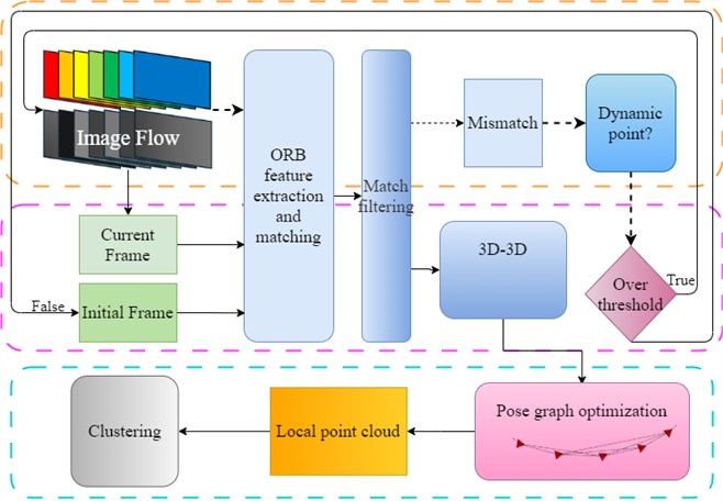
This study investigates visual SLAM in dynamic indoor environments. In the visual odometry module, it addresses the reduced accuracy of camera pose estimation caused by degraded data association due to moving objects. Within the mapping module, dynamic targets are generated and their 3D information is filtered to minimize environmental map contamination. Fig. 1 illustrates the workflow of the proposed visual SLAM method, which processes highly-dynamic image streams through feature extraction and matching optimization, dynamic feature labeling and removal, complete dynamic object identification, and a keyframe selection mechanism that incorporates dense reconstruction considerations. The system ultimately produces a static indoor scene point cloud map by integrating multi-stage dynamic filtering with spatial representation techniques.
3.1. Visual odometry for indoor dynamic environments
3.1.1. Optimization of feature matching
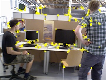
Feature matching, which establishes correspondences between feature points in consecutive images via descriptor comparison, is a fundamental component of visual odometry. In practice, however, erroneous matches often occur, degrading pose estimation accuracy. Traditional approaches typically rely on the RANSAC (RANdom Sample Consensus) [15] algorithm to mitigate mismatches. Nevertheless, in dynamic environments, conventional RANSAC is limited by fixed error thresholds and inefficient iterative sampling, resulting in suboptimal speed and accuracy. To overcome these challenges, this study employs the GMS (Grid-based Motion Statistics) [16] algorithm, which filters matches using a regional statistical model to retain motion-consistent correspondences. As shown in Fig. 2, the optimized approach markedly reduces the number of false matches.
Fig. 1System framework
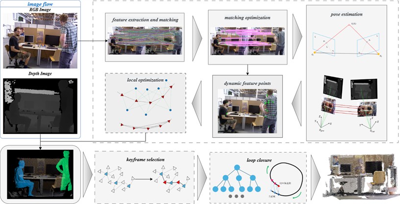
Fig. 2Optimized feature matching
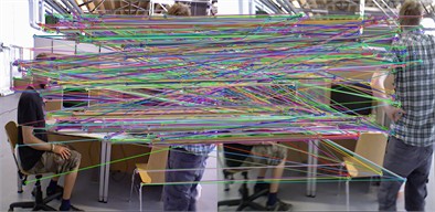
a) Brute-force
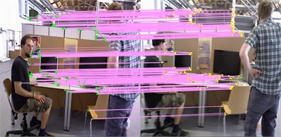
b) Ours
3.1.2. Dynamic feature point labeling
Based on the analysis of the feature matching methodology discussed previously, erroneous feature point matches can be categorized into two distinct types. The first type arises from feature descriptors exhibiting significant discrepancies yet still satisfying the minimum matching criteria, representing random errors. The second type comprises feature pairs with high descriptor similarity and small matching distances but lacking corroborating matches of the same type in their local neighborhood; these cases predominantly correspond to isolated dynamic feature points [16]. To address this issue, the proposed strategy selects erroneous matches with matching distances below a predefined threshold for validation against a pre-estimated geometric model. Specifically, the Euclidean distance between the transformed coordinates of the current point (via rotation) and its reference position is calculated. Matches that satisfy this distance threshold are subsequently classified as dynamic points.
As illustrated in Fig. 3, consider a spatial point with coordinates in the camera coordinate system of the current frame , corresponding to pixel coordinates . This point corresponds to a spatial point in the reference frame , where has pixel coordinates . According to the camera motion model, the coordinates of when back-projected into the reference frame are denoted as , which is obtained using Eq (1):
where denotes the rotation matrix from the current frame to the reference frame, and represents the translation vector. Both are derived from the feature matching set introduced in the previous subsection, combined with a specific camera pose estimation model, as illustrated in Fig. 4. is selected from the candidate dynamic point set and back-projected. Assuming that the spatial point lies on a moving object, this results in two visually similar feature points, and , occupying distinct spatial positions in the reference coordinate system. Ideally, the coordinates of and should coincide. However, the presence of dynamic objects introduces deviations between these coordinates, which are quantified by calculating the Euclidean distance between the two points. Denoting the coordinates of as and those of as , the distance between and can be computed using Eq. (2):
Fig. 3Determination of dynamic feature points
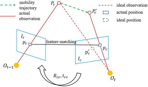
Let denote the threshold for identifying dynamic points, which is determined by comprehensively considering both camera observation errors and pose estimation inaccuracies. The candidate dynamic point set is generated from erroneous feature matches. These mismatches may include cases caused by static objects, where the corresponding spatial point distance variation significantly exceeds the threshold . To reduce false labeling of dynamic points, the maximum allowable error distance can be constrained by taking into account the sensor sampling frequency and the typical movement speeds of common indoor objects.
Fig. 4Filtering of dynamic feature points
a) Candidate dynamic feature points

b) Dynamic feature points
3.1.3. Initialization in dynamic scenarios
By integrating dynamic feature point identification and rejection methods, the system jointly optimizes the initial pose estimates of the visual SLAM system and the corresponding map points. During initialization, the system seeks to minimize dynamic features in the image stream to establish a stable initial map, while adaptively determining parameters required for subsequent clustering-based dynamic object detection based on this initialized map. The framework assumes minimal structural changes in environmental objects, allowing clustering parameters to be generated once during initialization and reused throughout operation.
In the first stage of initialization for binocular and RGB-D cameras, dynamic feature detection can be combined with dynamic feature point discrimination methods, introducing an additional step for selecting the first keyframe compared to monocular camera initialization. The overall workflow is illustrated in Fig. 5. After system startup, ORB features are extracted from the continuously input image stream, and feature matching is performed. For well-matched feature points, a 3D-3D motion model is used to estimate pose information. For mismatched feature points, motion consistency constraints are applied based on this pose information to determine whether they correspond to dynamic features. For frames containing dynamic features, point cloud structures are reconstructed, and adaptive DBSCAN is applied to determine clustering parameters, including radius and minimum sample count thresholds. These parameters are then directly used in subsequent clustering operations.
Fig. 5Flowchart of dynamic scene initialization
3.2. Map construction with dynamic object removal
3.2.1. Keyframe selection
Camera sensors typically sample the surrounding environment at frequencies of no less than 30 frames per second, resulting in visual SLAM systems having to process massive amounts of image frame data. If every frame were to indiscriminately contribute to map construction, it would impose excessive computational overhead on the SLAM system and generate significant data redundancy. Therefore, selecting representative images as keyframes provides an effective solution to mitigate this issue.
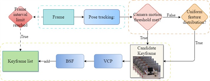
Current keyframe selection mechanisms typically rely on criteria such as image information content, frame overlap, or temporal intervals; however, they often fail to account for the influence of dynamic environments and lack sufficient representativeness. To address this, this section adopts the keyframe selection mechanism proposed in KeySLAM [17], transforming keyframe selection into a Vertex Coverage Problem (VCP) on an undirected graph and using the minimal solution of the model to select keyframes, effectively balancing environmental representation with keyframe quantity minimization. First, pose information for the current image frame is obtained from visual odometry, and the distance and attitude differences between the current frame and the previous frame are calculated. If these values exceed predefined thresholds, the current frame is added to the candidate keyframe container; if the thresholds are not exceeded but the feature points are evenly distributed across the image, the current frame is also added; otherwise, it is discarded. Next, it is determined whether the container contains the minimum number of frames required to construct the Vertex Coverage Problem. If the number of frames exceeds this minimum, an undirected graph is built based on the co-visibility relationships between image frames, and the minimal solution of this model is obtained. Subsequently, it is verified whether all keyframes are connected within the network. For any disconnected keyframes, a Breadth-First Search (BFS) is performed to establish bridge nodes, which are treated as keyframes and added to the container. Finally, considering the impact of dynamic feature points, dynamic feature detection is conducted on the selected keyframes; for keyframes containing dynamic features exceeding the maximum point threshold, replacement or enhancement is performed. The overall selection process is illustrated in Fig. 6.
Fig. 6Selection of keyframes
3.2.2. Dynamic target labeling
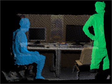
Starting from the dynamically labeled feature points obtained in visual odometry, moving objects in the scene are clustered, with each cluster representing a dynamic target, as illustrated in Fig. 8. The green feature points in Fig. 7(a) indicate dynamic points identified by visual odometry, whose 3D structures can be rapidly reconstructed using depth information. Fig. 7(b) shows two clustered dynamic targets in the local point cloud, exhibiting incomplete coverage compared to the image plane due to significant depth measurement errors in these regions caused by the depth camera.
DBSCAN (Density-Based Spatial Clustering of Applications with Noise) [18] is a density-based spatial clustering algorithm that is robust to noise. By defining density-connected sets as clusters, it ensures stable operation on noisy datasets and is unaffected by target shape constraints. Considering that DBSCAN’s time complexity depends on neighborhood point searches, constructing a K-D Tree index for the clustered dataset reduces distance-based search latency [19], thereby accelerating dynamic target identification and minimizing unnecessary cluster generation. The K-D Tree-accelerated DBSCAN clustering relies on two critical initialization parameters: the neighborhood radius and the minimum number of points in a neighborhood , whose selection directly impacts clustering quality and speed. Excessively small values may fragment a single target into multiple clusters, compromising dynamic target completeness and map quality, whereas excessively large values may cause oversegmentation by merging adjacent structures into dynamic targets, increasing computational load. To address parameter selection, this section employs the K-Nearest Neighbor (KNN) [20] algorithm to compute Euclidean distances between all point cloud points, forming a distance distribution matrix . For each row in this matrix, the average distance is calculated. Subsequently, the average number of neighboring points within -radius spheres across the point cloud determines .
Fig. 7Determine complete dynamic objectives

a) Dynamic feature points
b) Results of clustering
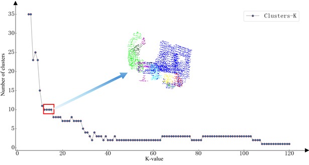
The aforementioned method generates candidate lists for the two critical parameters – neighborhood radius and minimum point threshold . To identify optimal parameters for the current scene data, DBSCAN is executed using paired values from corresponding positions in both candidate lists. Taking the scenario in Fig. 7(b) as an example, the relationship between cluster quantity and K-nearest neighbor values is illustrated in Fig. 8. Analysis reveals that the cluster count gradually stabilizes with increasing K-values, and the first stabilization interval is selected to determine the optimal and parameters.
Fig. 8Number of cluster classes graph
4. Experiments
4.1. Experimental data and evaluation criteria
This study employs the public RGB-D dataset [21], released in 2012 by the Computer Vision Group at the Technical University of Munich (TUM). The dataset contains 39 indoor sequences, with RGB and depth images captured by Microsoft Kinect sensors at a resolution of 640×480 pixels and a frame rate of 30 Hz. Depth data are obtained by projecting a random speckle pattern and analyzing its distortion to compute depth values. The raw depth maps have a resolution of 320×240 pixels; however, following hardware calibration and alignment with the color images, they are provided as 16-bit PNG files at 640×480 resolution. The effective sensing range of the depth camera spans from 0.8 m to 3.5 m, with optimal accuracy achieved between 1 m and 4 m. The depth measurement error along the Z-axis is approximately 1 cm. Ground-truth trajectory data are post-processed with a motion capture system, yielding absolute errors of less than 10 mm in position and 0.5° in orientation across the capture area.
The TUM dataset includes standard static scenes, structural and textured environments, and dynamic sequences. To evaluate the performance of the proposed visual SLAM scheme in indoor dynamic settings, five dynamic sequences were selected for testing, as shown in Fig. 9. Scene naming follows a specific convention: “freiburg3” indicates the sensor code; “sitting” refers to dynamic targets performing only minor movements, such as turning or making gestures; and “walking” denotes targets engaging in larger motions, such as walking back and forth. The suffixes “static”, “halfsphere”, “rpy” and “xyz” specify four different camera motion modes: the camera remains stationary, moves along a hemispherical trajectory with a diameter of 1 m, rotates about the roll, pitch, and yaw axes, or translates along the XYZ axes, respectively. For simplicity, “freiburg”, “halfsphere”, “rpy”, “sitting”, “walking” and “xyz” are abbreviated as “fr”, “h”, “r”, “s”, “w”, and “x” For example, the sequence “fr3/sitting_xyz” is denoted as “fr3/s/x” in this paper.
Experimental results are evaluated using Absolute Trajectory Error (ATE) [22] and Relative Pose Error (RPE) [22] to quantitatively assess the camera motion trajectory estimated by the visual SLAM system.
Fig. 9TUM RGB-D dataset

a) fr3/s/h

b) fr3/s/s

c) fr3/w/r

d) fr3/w/s

e) fr3/w/x
4.2. Experimental results and analysis
This section presents comparative experiments between the improved algorithm and classical approaches. In the first part, the TUM dataset with ground-truth trajectories is employed to evaluate the performance of the original ORB-SLAM2 and the proposed scheme using metrics such as ATE, RPE, and trajectory errors. Tables 1, 2, and 3 report the RMSE, mean, median, and standard deviation (S.D.) of these evaluation metrics in dynamic scenarios. These quantitative indicators effectively capture the accuracy, stability, and robustness of visual SLAM solutions, thereby enabling a comprehensive analysis and assessment of improvements in system localization performance.
In dynamic scenarios, the proposed method enhances localization performance by thoroughly detecting and eliminating dynamic feature points during system initialization and feature matching. In low-dynamic environments, ATE metrics show moderate improvements, with RMSE values reduced by an average of 37.68 %, although the overall enhancement remains limited. This limitation arises from the sparse distribution of dynamic points caused by minimal motion of dynamic targets. The mean and median values decrease by an average of 34.24 % and 27.78 %, respectively, while the standard deviation (S.D.) drops by 50.08 %, indicating a marked improvement in system stability. In high-dynamic scenarios, the RMSE of ATE metrics decreases by 77.57 % on average, demonstrating that the baseline method inevitably incorporates numerous dynamic feature points into data association, whereas the proposed approach effectively mitigates their impact to improve accuracy. The mean and median values are reduced by an average of 75.93 % and 72.62 %, respectively, with S.D. values declining by 83.07 %. Particularly significant improvements are observed in the fr3/w/x scenario, where camera motion occurs primarily along horizontal or vertical axes. In this case, dynamic objects remain relatively static with respect to the camera, rendering conventional RANSAC algorithms ineffective for dynamic point detection. The proposed method overcomes this limitation by integrating spatial distance verification through feature back-projection, enabling robust detection and removal of dynamic features and thereby substantially enhancing trajectory estimation accuracy and robustness.
Table 1Results of ATE
Scene | Evaluation index | fr3/s/h | fr3/s/s | fr3/w/r | fr3/w/s | fr3/w/x |
ORB-SLAM2 (m) | RMSE | 0.0378 | 0.0065 | 0.1471 | 0.0206 | 0.2952 |
Mean | 0.0335 | 0.0055 | 0.1324 | 0.0171 | 0.2594 | |
Median | 0.0281 | 0.0048 | 0.1239 | 0.0125 | 0.2455 | |
S.D. | 0.0174 | 0.0034 | 0.0640 | 0.0114 | 0.1409 | |
Ours (m) | RMSE | 0.0163 | 0.0053 | 0.0270 | 0.0081 | 0.0283 |
Mean | 0.0154 | 0.0047 | 0.0259 | 0.0073 | 0.0254 | |
Median | 0.0153 | 0.0043 | 0.0239 | 0.0067 | 0.0225 | |
S.D. | 0.0054 | 0.0023 | 0.0078 | 0.0034 | 0.0124 | |
Promotion (%) | RMSE | 56.82 | 18.55 | 81.62 | 60.67 | 90.41 |
Mean | 54.02 | 14.47 | 80.45 | 57.14 | 90.20 | |
Median | 45.59 | 9.98 | 80.73 | 46.31 | 90.82 | |
S.D. | 69.28 | 30.87 | 87.81 | 70.24 | 91.17 |
Tables 2 and 3 report the relative pose estimation errors between cameras in terms of translation and rotation, measured in meters and degrees, respectively. A combined analysis with Table 1 shows that the proposed method achieves an average RMSE reduction of 42.38 % for translation errors, with mean, median, and S.D. values improved by 26.47 %, 30.00 %, and 28.22 % on average. For rotation errors, the method achieves an average RMSE reduction of 26.57 %, while the mean, median, and S.D. values decrease by 27.97 %, 28.75 %, and 28.04 %, respectively.
Table 2Translation error of RPE
Scene | Evaluation index | fr3/s/h | fr3/s/s | fr3/w/r | fr3/w/s | fr3/w/x |
ORB-SLAM2 (m) | RMSE | 0.0089 | 0.0045 | 0.0074 | 0.0446 | 0.2906 |
Mean | 0.0071 | 0.0038 | 0.0052 | 0.0151 | 0.0082 | |
Median | 0.0058 | 0.0034 | 0.0040 | 0.0068 | 0.0079 | |
S.D. | 0.0053 | 0.0023 | 0.0053 | 0.0420 | 0.0042 | |
Ours (m) | RMSE | 0.0051 | 0.0031 | 0.0049 | 0.0385 | 0.0287 |
Mean | 0.0041 | 0.0026 | 0.0033 | 0.0125 | 0.0079 | |
Median | 0.0033 | 0.0023 | 0.0021 | 0.0054 | 0.0074 | |
S.D. | 0.0030 | 0.0016 | 0.0037 | 0.0318 | 0.0037 | |
Promotion (%) | RMSE | 42.91 | 31.44 | 33.60 | 13.86 | 90.12 |
Mean | 42.93 | 31.19 | 36.82 | 17.27 | 4.11 | |
Median | 43.82 | 32.06 | 48.10 | 20.61 | 5.38 | |
S.D. | 43.55 | 32.18 | 30.66 | 24.42 | 10.31 |
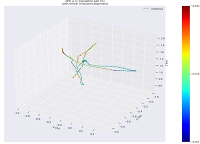
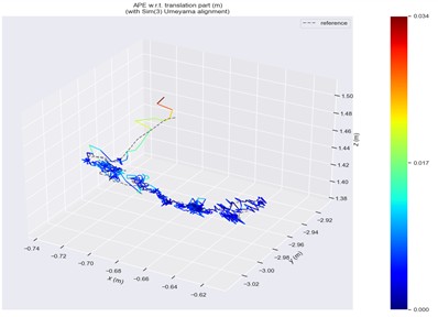
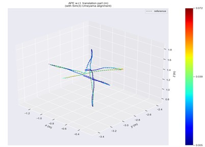
Trajectory error visualizations are provided to compare the original and improved methods. Figs. 10 to 14 present results from selected dynamic scenarios, showing that the proposed method achieves markedly better alignment with the ground-truth trajectories in high-dynamic cases (fr3/w/r, fr3/w/s, fr3/w/x). In particular, for the fr3/w/x sequence, the original method produces a maximum error of 0.639 m, whereas the improved method reduces this to 0.072 m. By contrast, in low-dynamic scenarios (fr3/s/h, fr3/s/s), the trajectory patterns of both methods appear visually similar, with only minor differences in color representation.
Table 3Rotation error of RPE
Scene | Evaluation index | fr3/s/h | fr3/s/s | fr3/w/r | fr3/w/s | fr3/w/x |
ORB-SLAM2 (deg) | RMSE | 0.3928 | 0.1588 | 0.8284 | 0.7587 | 0.9153 |
Mean | 0.3302 | 0.1349 | 0.5586 | 0.3266 | 0.5679 | |
Median | 0.2811 | 0.1137 | 0.4192 | 0.1881 | 0.4286 | |
S.D. | 0.2128 | 0.0838 | 0.6117 | 0.6848 | 0.7179 | |
Ours (deg) | RMSE | 0.2383 | 0.1500 | 0.4578 | 0.6110 | 0.6977 |
Mean | 0.1952 | 0.1212 | 0.2559 | 0.3356 | 0.3554 | |
Median | 0.1603 | 0.1019 | 0.2127 | 0.1912 | 0.2455 | |
S.D. | 0.1367 | 0.0754 | 0.3634 | 0.6098 | 0.4102 | |
Promotion (%) | RMSE | 39.32 | 5.52 | 44.74 | 19.47 | 23.78 |
Mean | 40.86 | 10.13 | 54.19 | –2.75 | 37.42 | |
Median | 42.97 | 10.43 | 49.26 | –1.66 | 42.72 | |
S.D. | 35.76 | 10.04 | 40.60 | 10.95 | 42.85 |
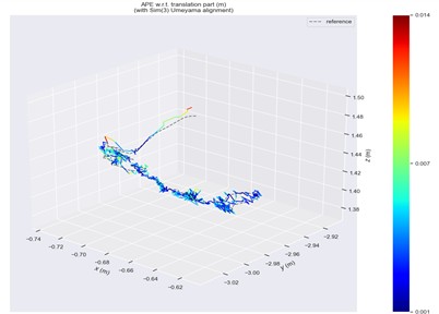
Fig. 10ATE in fr3/sitting/halfsphere scene
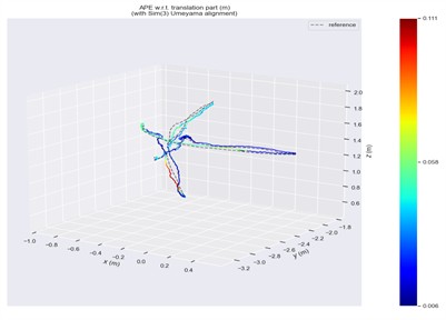
a) ORB-SLAM2
b) Ours
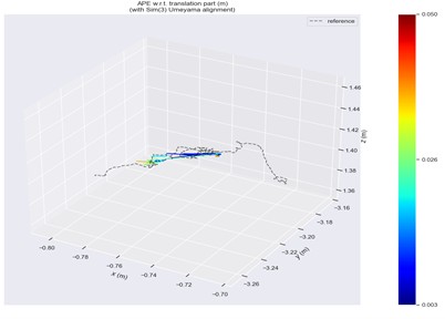
Fig. 11ATE in fr3/sitting/static scene
a) ORB-SLAM2
b) Ours
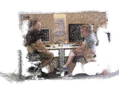
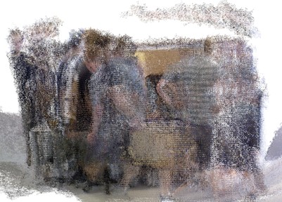
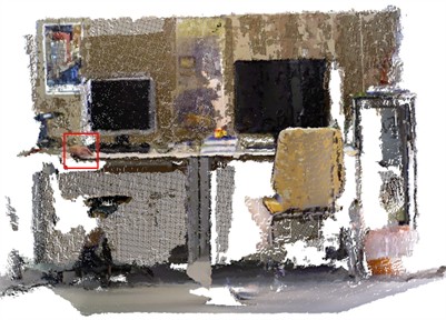
3D reconstruction results on the TUM RGB-D dataset are illustrated in Figs. 14 and 15. Since the original ORB-SLAM2 algorithm cannot directly generate dense point cloud maps, this study employs optimized keyframe poses for final scene reconstruction. In the low-dynamic scenario shown in Fig. 14, the original method reconstructs overall scene structures adequately but fails to detect and remove moving objects. By contrast, the improved method successfully localizes dynamic targets through detected dynamic points and eliminates them. In the high-dynamic scenario of Fig. 15, large object motions severely degrade inter-frame pose estimation in the original method, leading to maps contaminated by distorted dynamic human figures and cluttered structures, which provide little value for downstream tasks. The proposed method mitigates these issues by enhancing feature matching quality and pose estimation accuracy through dynamic feature detection in the visual odometry module, thereby preserving scene structural integrity. Nevertheless, dynamic object clustering may leave residual noise points due to partial occlusions. For instance, as highlighted by the red boxes in Figs. 15 and 16, discontinuous palm regions near tables remain visible in the final point cloud despite dynamic target removal.
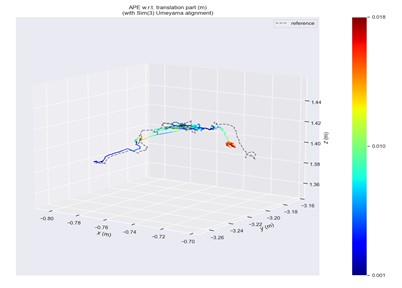
Fig. 12ATE in fr3/walking/rpy scene

a) ORB-SLAM2

b) Ours
Fig. 13ATE in fr3/walking/static scene
a) ORB-SLAM2
b) Ours
Fig. 14ATE in fr3/walking/xyz scene
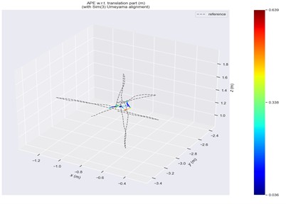
a) ORB-SLAM2
b) Ours
Fig. 15Reconstruction of the fr3/sitting/static scene
a) ORB-SLAM2

b) Ours
Fig. 16Reconstruction of the fr3/walking/xyz scene
a) ORB-SLAM2
b) Ours
5. Conclusions
To address the performance degradation of visual SLAM in indoor dynamic environments caused by moving objects, this study proposes a motion consistency-constrained framework that incorporates dynamic feature elimination into both the visual odometry and mapping modules.
Experiments on the TUM RGB-D dataset demonstrate substantial improvements over ORB-SLAM2. In high-dynamic scenarios, the proposed method reduces the Absolute Trajectory Error (ATE) root mean square error (RMSE) by an average of 77.57 %, while the Relative Pose Error (RPE) translation and rotation errors decrease by 42.38 % and 26.57 %, respectively. Notably, in the fr3/w/x scenario – where dynamic objects and the camera remain relatively static – the maximum trajectory error is reduced from 0.639 m to 0.072 m, effectively overcoming the limitations of traditional approaches.
For mapping, the framework enhances keyframe selection – modeled as a Vertex Cover Problem – and applies DBSCAN clustering to eliminate dynamic objects. This ensures that dense point cloud reconstructions preserve static structures (e.g., walls and furniture), in contrast to baseline methods that yield distorted, dynamically contaminated maps.
Nevertheless, limitations remain. Residual noise persists in areas with occluded dynamic features, and effectiveness is reduced when handling textureless or fast-moving targets. Future work will integrate semantic segmentation, refine clustering parameter selection, and reduce computational overhead to improve real-time applicability.
References
-
J. Kunhoth, A. Karkar, S. Al-Maadeed, and A. Al-Ali, “Indoor positioning and wayfinding systems: a survey,” Human-centric Computing and Information Sciences, Vol. 10, No. 1, p. 18, May 2020, https://doi.org/10.1186/s13673-020-00222-0
-
W. F. A. Wan Aasim, M. Okasha, and W. F. Faris, “Real-time artificial intelligence based visual simultaneous localization and mapping in dynamic environments – a review,” Journal of Intelligent and Robotic Systems, Vol. 105, No. 1, p. 15, May 2022, https://doi.org/10.1007/s10846-022-01643-y
-
Z. Song, W. Su, H. Chen, M. Feng, J. Peng, and A. Zhang, “VSLAM optimization method in dynamic scenes based on YOLO-fastest,” Electronics, Vol. 12, No. 17, p. 3538, Aug. 2023, https://doi.org/10.3390/electronics12173538
-
Y. Wang, Y. Zhang, L. Hu, G. Ge, W. Wang, and S. Tan, “Improved feature point extraction method of VSLAM in low-light dynamic environment,” Electronics, Vol. 13, No. 15, p. 2936, Jul. 2024, https://doi.org/10.3390/electronics13152936
-
G. Yadav, S. Maheshwari, and A. Agarwal, “Contrast limited adaptive histogram equalization based enhancement for real time video system,” in International Conference on Advances in Computing, Communications and Informatics (ICACCI), pp. 2392–2397, Sep. 2014, https://doi.org/10.1109/icacci.2014.6968381
-
J. Lv et al., “MOLO-SLAM: A Semantic SLAM for accurate removal of dynamic objects in agricultural environments,” Agriculture, Vol. 14, No. 6, p. 819, May 2024, https://doi.org/10.3390/agriculture14060819
-
R. Mur-Artal and J. D. Tardos, “ORB-SLAM2: an open-source SLAM system for monocular, stereo, and RGB-D cameras,” IEEE Transactions on Robotics, Vol. 33, No. 5, pp. 1255–1262, Oct. 2017, https://doi.org/10.1109/tro.2017.2705103
-
Z. Zhu et al., “NICE-SLAM: neural implicit scalable encoding for SLAM,” in 2022 IEEE/CVF Conference on Computer Vision and Pattern Recognition (CVPR), pp. 12776–12786, Jun. 2022, https://doi.org/10.1109/cvpr52688.2022.01245
-
B. Mildenhall, P. P. Srinivasan, M. Tancik, J. T. Barron, R. Ramamoorthi, and R. Ng, “NeRF: representing scenes as neural radiance fields for view synthesis,” Communications of the ACM, Vol. 65, No. 1, pp. 99–106, Dec. 2021, https://doi.org/10.1145/3503250
-
C. Yan et al., “GS-SLAM: dense visual SLAM with 3D Gaussian splatting,” in 2024 IEEE/CVF Conference on Computer Vision and Pattern Recognition (CVPR), pp. 19595–19604, Jun. 2024, https://doi.org/10.1109/cvpr52733.2024.01853
-
B. Kerbl, G. Kopanas, T. Leimkuehler, and G. Drettakis, “3D Gaussian splatting for real-time radiance field rendering,” ACM Transactions on Graphics, Vol. 42, No. 4, pp. 1–14, Jul. 2023, https://doi.org/10.1145/3592433
-
S. Wei, S. Wang, H. Li, G. Liu, T. Yang, and C. Liu, “A semantic information-based optimized vSLAM in indoor dynamic environments,” Applied Sciences, Vol. 13, No. 15, p. 8790, Jul. 2023, https://doi.org/10.3390/app13158790
-
C. Yu, C. Gao, J. Wang, G. Yu, C. Shen, and N. Sang, “BiSeNet V2: bilateral network with guided aggregation for real-time semantic segmentation,” arXiv:2004.02147, Jan. 2020, https://doi.org/10.48550/arxiv.2004.02147
-
R. Qiu, Y. He, F. R. Yu, and G. Zhou, “SPP-SLAM: dynamic visual SLAM with multiple constraints based on semantic masks and probabilistic propagation,” in 2024 IEEE Wireless Communications and Networking Conference (WCNC), pp. 1–6, Apr. 2024, https://doi.org/10.1109/wcnc57260.2024.10570745
-
M. A. Fischler and R. C. Bolles, “Random sample consensus: a paradigm for model fitting with applications to image analysis and automated cartography,” Communications of the ACM, Vol. 24, No. 6, pp. 381–395, Jun. 1981, https://doi.org/10.1145/358669.358692
-
J. Bian, W.-Y. Lin, Y. Matsushita, S.-K. Yeung, T.-D. Nguyen, and M.-M. Cheng, “GMS: grid-based motion statistics for fast, ultra-robust feature correspondence,” in 2017 IEEE Conference on Computer Vision and Pattern Recognition (CVPR), pp. 2828–2837, Jul. 2017, https://doi.org/10.1109/cvpr.2017.302
-
K. M. Han and Y. J. Kim, “KeySLAM: robust RGB-D camera tracking using adaptive VO and optimal key-frame selection,” IEEE Robotics and Automation Letters, Vol. 5, No. 4, pp. 6940–6947, Oct. 2020, https://doi.org/10.1109/lra.2020.3026964
-
A. Ram, A. Sharma, A. S. Jalal, A. Agrawal, and R. Singh, “An enhanced density based spatial clustering of applications with noise,” in 2009 IEEE International Advance Computing Conference (IACC 2009), pp. 1475–1478, Mar. 2009, https://doi.org/10.1109/iadcc.2009.4809235
-
Y. Chen, W. Ruys, and G. Biros, “KNN-DBSCAN: a DBSCAN in high dimensions,” ACM Transactions on Parallel Computing, Vol. 12, No. 1, pp. 1–27, Mar. 2025, https://doi.org/10.1145/3701624
-
Z. Zhang, “Introduction to machine learning: k-nearest neighbors,” Annals of Translational Medicine, Vol. 4, No. 11, pp. 218–218, Jun. 2016, https://doi.org/10.21037/atm.2016.03.37
-
J. Sturm, N. Engelhard, F. Endres, W. Burgard, and D. Cremers, “A benchmark for the evaluation of RGB-D SLAM systems,” in 2012 IEEE/RSJ International Conference on Intelligent Robots and Systems (IROS 2012), pp. 573–580, Oct. 2012, https://doi.org/10.1109/iros.2012.6385773
-
Z. Zhang and D. Scaramuzza, “A tutorial on quantitative trajectory evaluation for visual(-Inertial) Odometry,” in 2018 IEEE/RSJ International Conference on Intelligent Robots and Systems (IROS), pp. 7244–7251, Oct. 2018, https://doi.org/10.1109/iros.2018.8593941
About this article

The authors have not disclosed any funding.
The datasets generated during and/or analyzed during the current study are available from the corresponding author on reasonable request.
Shan Zhou contributed the central idea, implemented most of algorithms, and wrote the initial draft of the paper. Shuangfeng Wei contributed to refining the ideas, and finalizing this paper. Shangxing Wang implemented feature matching algorithms, and writing the corresponding part of this paper. Ming Guo and Jianghong Zhao was responsible for data collecting and pre-processing.
The authors declare that they have no conflict of interest.
