Pure IMU localization for intelligent platforms with CNN adaptive invariant extended Kalman filter noise fusion

Han, J.; Hou, Z. W.; Zhang, T.; Wu, S. X.; Xu, D. Y.

doi:10.21595/jve.2025.24765

Journal of Vibroengineering

Browse Journal

Submit article

Published: 13 April 2025

Check for updates

Pure IMU localization for intelligent platforms with CNN adaptive invariant extended Kalman filter noise fusion

J. Han¹

Z. W. Hou²

T. Zhang³

S. X. Wu⁴

D. Y. Xu⁵

^{1, 4, 5}School of Information Science and Engineering, Chongqing Jiaotong University, Chongqing, 400074, China

²Institute of Future Civil Engineering Sciences and Technology, Chongqing Jiaotong University, Chongqing, 400074, China

³Chongqing City Investment Infrastructure Construction Co., Ltd., Chongqing, 400010, China

Corresponding Author:

Z. W. Hou

Cite the article Download PDF

Article in Press

Downloads 79

Abstract

In the context of intelligent vehicles, low- and medium- precision Inertial Measurement Units (IMU) are plagued by high levels of noise and considerable output uncertainly. When positioning and attitude estimation rely solely on IMU data, errors rapidly accumulate over time. To address this issue, this paper introduces a Convolutional Neural Network (CNN)-based noise-adaptive invariant extend Kalman filter (IEKF) vehicle localization. The proposed approach develops CNN models tailored for IMU measurement data as well as the process noise and observation noise in the IEKF. An enhanced CNN architecture and convolution mechanism are designed to dynamically adjust the covariance matrices associated with both process noise and observation noise in response to varying IMU input. This integration with IEKF principles ensures real-time positioning while achieving high accuracy in position prediction. The proposed method was tested and validated on 16 IMU sequences from the KITTI dataset, resulting in a relative translation error performance improvement ranging from a minimum of 10 % to a maximum of 24 % when compared to four existing methods. Additionally, its performance was further evaluated through various metrics including cumulative distribution of errors, root mean square error, and absolute position error. Trajectory tracking experiments further demonstrated that the proposed method produces smoother localization curves and more stable positioning performance.

Pure IMU localization for intelligent platforms with CNN adaptive invariant extended Kalman filter noise fusion

Highlights

The proposed CNN enhanced adaptive IEKF method reduces the relative translation errors by up to 23.9%, 14.8%, 9.8%, and 13.3%, respectively.
CNN's local receptive fields enable more precise modeling of noise than LSTM.
This method can mitigate the error of low-cost IMUs and provide a cost-effective solution for intelligent vehicles positioning.
CNN outperforms LSTM in inertial localization by effectively capturing spatial correlations in IMU sequences processing.
One-dimensional improved CNN is used to dynamically adjust the process and measurement noise of IEKF.

1. Introduction

Micro-Electro-Mechanical System Inertial Measurement Units (MEMS IMUS) are extensively employed in localization applications due to their simple structure, high independence, and low cost. While IMUs can provide stable positioning accuracy over shout durations, their errors accumulate over time, leading to divergent localization results [1]. Conversely, high-precision IMUs are limited by their elevated costs, rendering them unsuitable for civilian applications. To facilitate the widespread adoption of low-cost IMUs, it is essential to address their systematic errors through integration with other sensors or the application of deep learning techniques. Sensor-based approaches frequently utilize Kalman filtering to combine Global Navigation Satellite Systems (GNSS) with IMUs, compensating for limitations of both systems [2-4] and ensuring positional accuracy. However, synchronization errors and GNSS signal instability continue to pose challenges-particularly in demanding scenarios such as long tunnels or densely built urban environments, leaving the issue of IMU error accumulation unresolved. The fusion of LIDAR, odometry, Ultra-Wideband (UWB), and cameras with IMUs has the potential to enhances the robustness and stability of navigation systems within complex and unknown environments [5-8], but the hardware costs and computational resource requirements still remain significant challenges.

In term of deep learning, their application in IMU-based localization has significantly enhanced both positioning accuracy and reliability. Currently, deep learning-driven pure IMU localization methods can be broadly classified into two categories. One approach fully integrates deep learning with IMU without relying on filtering, by predicting the velocity vector to partially correct acceleration and adjust displacement [9]. Regarding the incorporation of attention mechanisms, Zhu et al. [10] introduced normalization modules and convolutional attention blocks into a residual network to enhance the model's capacity for learning spatiotemporal features. Meanwhile, Brotchie et al. [11] employed two deep inertial odometry frameworks that leverage self-attention to capture long-term dependencies in IMU data. In terms of model lightweighting, Zeinali et al. [12] integrated depthwise separable convolutions into their regression model, significantly reducing the number of training parameters. Similarly, Lai et al. [13] replaced traditional convolution operations with Mixer layers to more efficiently capture input data dependencies, resulting in a lighter-weight model. With respect to model fusion, Wang et al. [14] proposed a Spatiotemporal Co-Attention Hybrid Neural Network (SC-HNN) that combines spatial and temporal attention mechanisms to extract both local and global features for velocity prediction. Additionally, Rao et al. [15] combined ResNet with Transformer architectures to enhance the model’s ability to capture spatial context within IMU sequences, thereby improving prediction accuracy for both velocity and trajectory. In displacement prediction tasks, Jayanth et al.’s EqNIO model [16] incorporates the inherent physical rotational reflection symmetry present in IMU data to bolster the generalization capabilities of their framework. It is important to note that these methods do not rely on any external sensors; however, they necessitate highly accurate labels for training ground truth and are heavily dependent on device orientation for transforming IMU data into a global coordinate system.

Other category of positioning methods combines deep learning with Kalman filtering, leveraging physical motion processes to provide more stable and smoother positioning results compared to methods without filtering. Lin et al. [17] proposed a monocular visual-inertial odometry method based on convolutional neural networks with extended Kalman filtering (EKF) for more accurate pose estimation. Chen et al. [18] created a neural Kalman dynamics model that uses visual-inertial odometry for motion prediction, enabling the extraction of relevant features from rich input data. Damagatla and Atia [3] employed EKF combined with deep learning to estimate position, attitude, and velocity values when GNSS signals are available, thus addressing environments without GNSS signals, such as indoors. To overcome data limitations, Akmalioglu et al. [19] proposed a method based on adversarial training and adaptive visual-inertial odometry, which has demonstrated significant potential in visual-inertial navigation due to its superior performance. The above methods effectively reduce positioning errors by integrating high-precision sensors, but synchronization errors between sensors remain a challenge to resolve effectively. Liu et al. [20] employed a CNN to regress relative displacement and uncertainty between two time steps, integrating them into the EKF as observations for state estimation of orientation, velocity, position and IMU biases. This method also extends the two-dimensional localization problem to three-dimensional state estimation. An approach combined magnetic field gradient-based EKF with bidirectional long short-term memory (Bi-LSTM) networks to improve object motion velocity estimation in [21]. The improved dilated convolutional network was introduced in [22] aimed at calibrating and compensating for IMU gyroscope drift. In [23], the separate noise-adaptive model was designed for observation and process noise by employing CNN and LSTM networks, further enhancing localization accuracy. Nevertheless, the incorporation of LSTM results in increased training time and a slower convergence rate, leading to trajectories that exhibit a lack of smoothness and limited improvements in accuracy for shorter test sequences. The above method using IMU signals as inputs to neural network models does not sufficiently address the real-time requirements essential for effective position prediction.

This paper addresses the challenge of manually configuring observation noise and process noise during state updates in Kalman filtering, particularly in relation to the dynamic characteristics of wheeled vehicles. Instead of relying on manual settings, this research investigates adaptive adjustments based on IMU data input. While incorporating LSTM networks increases model complexity, the improvement in localization accuracy is marginal [23]. To achieve smoother localization trajectories and enhanced positioning accuracy, we propose a CNN-integrated noise-adaptive pure IMU IEKF, which incorporates pseudo-measurement information. The details are as follows: (1) deeper one-dimensional convolutional neural network (1D-CNN) architectures are developed to adaptively modify the covariance matrices associated with process noise and observation noise. (2) To ensure real-time position prediction capabilities, the convolution method is refined based on the principles of causal convolution [24] and dilated convolution [25]. (3) An experimental framework based on KITTI dataset [26] is designed, and the effectiveness of the proposed method is verified according to the relevant evaluation indexes. The remainder of this article is organized as follows. We first describe inertial localization with deep learning related methods in Section II. In Section III, we will introduce the IMU model and positioning model of wheeled vehicle motion. Section IV builds upon the models described in the previous section, utilizing the IEKF in combination with IMU outputs to generate vehicle position, orientation, and velocity information. Additionally, deep learning is employed to dynamically adapt the process noise covariance matrix and observation noise covariance matrix within the IEKF. Section V presents the performance of the proposed method on the KITTI dataset. Finally, the conclusion section provides a summary of our work.

2. Pure IMU modeling and localization

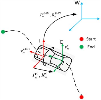
In the IMU localization model for wheel vehicles, three coordinate systems are involved: the IMU sensor coordinate system, the vehicle coordinate system, and the world coordinate system. The mapping between these coordinate systems are depicted in Fig. 1.

Fig. 1Coordinate system of wheeled vehicle in IMU positioning model

2.1. IMU modeling

A pure inertial localization system achieves positioning tasks by integrating angular velocity and acceleration. However, the IMU provides angular velocity and acceleration data with bias and noise [27], as shown below:

1

\begin{array}{l} w_{n}^{I M U} = w_{n} + b_{n}^{w} + w_{n}^{w}, \\ a_{n}^{I M U} = a_{n} + b_{n}^{a} + w_{n}^{a}, \end{array}

where, $b_{n}^{w}$ and $b_{n}^{a}$ represent time-varying zero biases, while $w_{n}^{w}$ and $w_{n}^{a}$ denote zero-mean Gaussian noise. The time-varying zero biases follow a random walk model, which describes the stochastic movement of random variables over a series of discrete time points. Its mathematical expression is as follows:

2

\begin{array}{l} b_{n + 1}^{w} = b_{n}^{w} + w_{n}^{b_{w}}, \\ b_{n + 1}^{a} = b_{n}^{a} + w_{n}^{b_{a}}, \end{array}

where $w_{n}^{b_{w}}$ and $w_{n}^{b_{a}}$ is zero-mean Gaussian noise. The kinematic model of the IMU can be expressed:

3

\begin{array}{l} R_{n + 1}^{I M U} = R_{n}^{I M U} e x p ((w_{n} d t)_{x}), \\ v_{n + 1}^{I M U} = v_{n}^{I M U} + (R_{n}^{I M U} a_{n} + g) d t, \\ p_{n + 1}^{I M U} = p_{n}^{I M U} + v_{n}^{I M U} d t, \end{array}

where $R_{n}^{I M U} \in S O (3)$ is a 3×3 rotation matrix representing the current orientation of the IMU, mapping from the IMU sensor coordinate system to the world coordinate system. $v_{n}^{I M U}$ is a 1×3 vector representing the velocity of the IMU at the current time. $R_{n}^{I M U}$ represent the position of the IMU within the world coordinate system. $d t$ denotes the time interval between two discrete sampling moments, $w_{n}$ and $a_{n}$ is the true angular velocity and acceleration, respectively, while g signifies a known constant corresponding to gravitational acceleration. $(s)_{x}$ refers to a skew-symmetric matrix associated with the cross product of vector $s \in R^{3}$ . Utilizing the above equations, the IMU outputs, including position, velocity, and attitude are transformed into the global coordinate system.

2.2. Localization modeling

Given the initial variables $(R_{0}^{I M U}, v_{0}^{I M U}, P_{0}^{I M U})$ , real-time dead reckoning in the world coordinate system is performed using the IMU-measured angular velocity $w_{n}^{I M U}$ and acceleration $a_{n}^{I M U}$ to localize the vehicle. This involves estimating the state variables of the IMU and the vehicle at time $n$ :

4

x_{n} = (R_{n}^{I M U}, v_{n}^{I M U}, p_{n}^{I M U}, b_{n}^{w}, b_{n}^{a}, R_{n}^{c}, p_{n}^{c}),

where $R_{n}^{c} \in R^{3}$ represents the orientation of the vehicle coordinate system, mapping the IMU coordinate system to the vehicle coordinate system. $p_{n}^{c} \in R^{3}$ denotes the position of the origin of the IMU coordinate system relative to the origin of the vehicle coordinate system, i.e., the lever arm between the IMU and the vehicle. Since the connection between the IMU and the vehicle is rigid, $R_{n}^{c}$ and $p_{n}^{c}$ can be approximated as constants, expressed as follows:

5

\begin{array}{l} R_{n + 1}^{c} = R_{n}^{c} e x p ({(w_{n}^{R^{c}} d t)}_{x}), \\ p_{n + 1}^{c} = p_{n}^{c} + w_{n}^{p^{c}}, \end{array}

where $w_{n}^{R^{c}}$ and $w_{n}^{p^{c}}$ represent zero-mean Gaussian noise with small covariance matrices, describing minor vibrations in the lever arm connecting the IMU and the vehicle. Using Eq. (5), the velocity, position, and other information calculated by the IMU are aligned with the velocity, position, and other information of the vehicle.

3. Noise adaptive IMU filtering method based on CNN

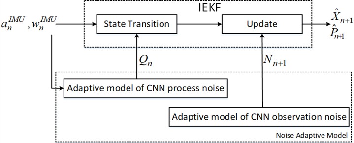
The overall framework of the method that integrates CNN-based adaptive adjustment of IEKF noise is illustrated in Fig. 2. The acceleration and angular velocity measurements from the IMU are separately input into both the IEKF and the noise-adaptive model. This noise-adaptive model dynamically generates the process noise and observation noise covariance matrices required by the IEKF filter, based on real-time IMU signal measurements. By replacing manual configuration with dynamic adjustment, the IMU signal measurements are combined with the IEKF filter principles to obtain the optimal estimation of the system state and covariance matrices.

Fig. 2Overall block diagram

3.1. IEKF principle

3.1.1. State transition equation

The state transition equation of the state variable $x_{n}$ can be easily constructed from Eqs. (2-3) and Eq. (5), and its mathematical expression is as follows:

6

x_{n + 1} = f (x_{n}, u_{n}) + w_{n},

where $u_{n}$ represents input variables, consisting of angular velocity $w_{n}^{I M U}$ and acceleration $a_{n}^{I M U}$ . $w_{n}$ is a vector composed of noise terms $w_{n}^{w}$ , $w_{n}^{a}$ , $w_{n}^{b_{w}}$ , $w_{n}^{b_{a}}$ , $w_{n}^{R^{c}}$ and $w_{n}^{p^{c}}$ , representing zero-mean Gaussian noise with a covariance matrix $Q_{n}$ Due to the nonlinearity of the state equations, linearization is required, according to [28], the state can be decomposed into three Lie groups: $χ_{n}^{I M U} = (R_{n}^{I M U}, v_{n}^{I M U}, p_{n}^{I M U})$ , mapped to $S E_{2} (3)$ , $b_{n} = {[{(b_{n}^{w})}^{T}, {(b_{n}^{a})}^{T}]}^{T} \in R^{6}$ , treated as a Lie group; $p_{n}^{c} \in R^{3}$ and $R_{n}^{c} \in R^{3}$ , mapped to $S O (3)$ . The linearized error is then expressed in vector form:

7

e_{n} = {[(ξ_{n}^{I M U})^{T} {(e_{n}^{b})}^{T} {(ξ_{n}^{R^{c}})}^{T} {(e_{n}^{p^{c}})}^{T}]}^{T} ~ N (0, P_{n}),

where $e_{n} \in R^{21}$ , $P_{n} \in R^{21 \times 21}$ . Each linearized error is mapped to the system state and multiplied by the elements of the system state space, resulting in the following update estimation:

8

\begin{array}{l} χ_{n}^{I M U} = e x p_{S E_{2} (3)} (ξ_{n}^{I M U}) {\hat{χ}}_{n}^{I M U}, \\ b_{n} = {\hat{b}}_{n} + e_{n}^{b}, \\ R_{n}^{c} = e x p_{S O (3)} (ξ_{n}^{R^{c}}) {\hat{R}}_{n}^{c}, \\ p_{n}^{c} = {\hat{p}}_{n}^{c} + e_{n}^{p^{c}}, \end{array}

where $χ_{n}^{I M U}$ , $b_{n}$ , $R_{n}^{c}$ and $p_{n}^{c}$ represent the estimated system state variables.

During the state transition phase, given an initial estimate and assuming $w_{n} = 0$ , the estimations are updated using Eq. (6). The corresponding covariance matrix is updated:

9

P_{n + 1} = F_{n} P_{n} F_{n}^{T} + G_{n} Q_{n} G_{n}^{T},

where $P_{n}$ represents the covariance matrix of the state variables at time $n$ , and $F_{n}$ , $G_{n}$ denote the Jacobian matrices of $x_{n}$ , $u_{n} f (x_{n}, u_{n})$ with respect to. These are computed:

10

F_{n} = I_{21 \times 21} + [\begin{matrix} 0_{3} & 0_{3} & 0_{3} & - R_{n}^{I M U} & 0_{3} & 0_{3 \times 6} \\ (g)_{\times} & 0_{3} & 0_{3} & - (v_{n}^{I M U})_{\times} R_{n}^{I M U} & - R_{n}^{I M U} & 0_{3 \times 6} \\ 0_{3} & I_{3} & 0_{3} & - (p_{n}^{I M U})_{\times} R_{n}^{I M U} & 0_{3} & 0_{3 \times 6} \\ 0_{12 \times 21} \end{matrix}],

11

G_{n} = [\begin{matrix} R_{n}^{I M U} & 0_{3 \times 3} & 0_{3 \times 12} \\ {(v_{n}^{I M U})}_{\times} R_{n}^{I M U} & R_{n}^{I M U} & 0_{3 \times 12} \\ {(p_{n}^{I M U})}_{\times} R_{n}^{I M U} & 0_{3 \times 3} & 0_{3 \times 12} \\ 0_{12 \times 3} & 0_{12 \times 3} & I_{12 \times 12} \end{matrix}] d t .

3.1.2. Observation equation

Considering three different coordinate systems, the vehicle speed in the vehicle coordinate system is represented:

12

v_{n}^{c} = [\begin{matrix} v_{n}^{f o r} \\ v_{n}^{l a t} \\ v_{n}^{n p} \end{matrix}] = {(R_{n}^{c})}^{T} {(R_{n}^{I M U})}^{T} v_{n}^{I M U} + {(w_{n})}_{\times} p_{n}^{c},

where $v_{n}^{f o r}$ , $v_{n}^{l a t}$ and $v_{n}^{u p}$ represent the vehicle’s forward velocity, lateral velocity, and vertical velocity, respectively. In the vehicle coordinate system, the lateral and vertical velocities can be assumed to be approximately zero. Thus, the system's observation equations can be specifically expressed:

13

y_{n + 1} = [\begin{array}{l} y_{n + 1}^{l a t} \\ y_{n + 1}^{u p} \end{array}] = [\begin{array}{l} y_{n + 1}^{l a t} + n_{n + 1}^{l a t} \\ y_{n + 1}^{u p} + n_{n + 1}^{u p} \end{array}] = [\begin{array}{l} y_{n + 1}^{l a t} \\ y_{n + 1}^{u p} \end{array}] + n_{n + 1},

where $n_{n + 1}$ represents observation noise following a zero-mean Gaussian distribution, with a covariance matrix $N_{n + 1} \in R^{2 \times 2}$ , the measurements are $y_{n + 1}^{l a t} = y_{n + 1}^{u p} = 0$ .

Based on Eq. (12-13), the Jacobian Matrix $H_{n + 1}$ of the measurement $y_{n + 1}$ with respect to the linearized error Eq. (7) is given by:

14

H_{n} = A [\begin{array}{l} 0_{3 \times 3} & {(R_{n}^{I M U})}^{T} & 0_{3 \times 3} & - {(p_{n}^{c})}_{\times} & 0_{3 \times 3} & B & C \end{array}],

where $A$ , $B$ and $C$ is:

15

\begin{array}{l} A = [\begin{array}{l} I_{2} & 0_{2} \end{array}], \\ B = {(R_{n}^{c})}^{T} {(R_{n}^{I M U})}^{T} {(v_{n}^{I M U})}_{\times} \\ C = - {(w_{n}^{I M U} - b_{n}^{w})}_{\times} . \end{array},

3.1.3. IEKF update steps

The IEKF method updates the system state ${\hat{x}}_{n + 1}^{+}$ and covariance matrix $P_{n + 1}^{+}$ as follows: Firstly, using Eq. (9) and Eq. (14), the Kalman gain is calculated:

16

S = (H_{n + 1} P_{n + 1} H_{n + 1}^{T} + N_{n + 1}), K = \frac{P_{n + 1} H_{n + 1}^{T}}{S} .

Secondly, the state is updated for Eq. (8):

17

\begin{array}{l} e^{+} = K (y_{n + 1} - {\hat{y}}_{n + 1}), \\ χ_{n + 1}^{I M U +} = e x p_{S E_{2} (3)} (ξ_{n}^{I M U}) {\hat{χ}}_{n + 1}^{I M U}, \\ b_{n + 1}^{+} = b_{n + 1} + e^{b +}, \\ {\hat{R}}_{n + 1}^{c +} = e x p_{S O (3)} (ξ^{R^{\in} +}) {\hat{R}}_{n + 1}^{c}, \\ {\hat{p}}_{n + 1}^{c +} = {\hat{p}}_{n + 1}^{c} + e^{p^{c} +} . \end{array}

Finally, the covariance matrix is updated as:

18

P_{n + 1}^{+} = (I_{21} - K H_{n + 1}) P_{n + 1} .

3.2. Adaptive model of CNN process noise

In the state transition equations of the IEKF, there exists a process noise covariance matrix $Q_{n}$ . Typically, this covariance matrix is assigned a fixed value based on empirical knowledge acquire by researchers. In this work, the IMU signals are used as input to design a noise-adaptive model for the process noise. This model enables the automatic adjustment of the parameters within the process noise covariance matrix in response to varying IMU signal inputs, thereby facilitating an adaptive modification of the process noise within the IEKF.

The neural network structure of the noise-adaptive model for process noise is shown in Fig. 3.

Its input is the IMU sensor values $u_{n} = [a_{n}^{T}, w_{n}^{T}] \in R^{6}$ , where $a_{n} = {[a_{x n}, a_{y n}, a_{z n}]}^{T}$ , $w_{n} = {[w_{x n}, w_{y n}, w_{z n}]}^{T}$ . The output is a 6-dimensional vector $q_{n}$ , specifically refers to $q_{n} = {[q_{n}^{w}, q_{n}^{a}, q_{n}^{b_{w}}, q_{n}^{b_{a}}, q_{n}^{R^{c}}, q_{n}^{p^{c}}]}^{T} \in R^{6}$ , which ultimately forms the process noise covariance matrix. The calculation formula is:

19

\{\begin{array}{l} Q_{n} = d i a g (\sum_{1}, \sum_{2}, \sum_{3}, \sum_{4}, \sum_{5}, \sum_{6}), \\ \sum_{1} = σ_{w}^{2} 1 0^{β t a n h (q_{n}^{w})}, \\ \sum_{2} = σ_{a}^{2} 1 0^{β t a n h (q_{n}^{a})}, \\ \sum_{3} = σ_{b_{w}}^{2} 1 0^{β t a n h (q_{n}^{b_{w}})}, \\ \sum_{4} = σ_{b_{a}}^{2} 1 0^{β t a n h (q_{n}^{b_{a}})}, \\ \sum_{5} = σ_{R^{c}}^{2} 1 0^{β t a n h (q_{n}^{R^{c}})}, \\ \sum_{6} = σ_{p^{c}}^{2} 1 0^{β t a n h (q_{n}^{p^{c}})}, \end{array}

where $σ$ represents the initialization parameter of the process noise covariance, and $β \in R > 0$ is the covariance inflation factor. Tanh is a commonly used activation function in neural networks, which constrains the input values to the range [–1, 1].

The process noise adaptive model employs a convolutional neural network (CNN)-based architecture, consisting of seven layers: an input layer, five hidden layers (designated as layer 1 through layer 5), and an output layer. The input layer receives acceleration and angular velocity data from the IMU sensor, which are processed through multiple convolutional layers. The hidden layers utilize the Relu activation function to progressively extract features from the incoming data. To ensure real-time performance, the model employs causal convolution, which ensures that the model’s decisions rely only on the current and past data without accessing future information, thus adhering to the causality inherent in time-series data. The last convolutional layer incorporates dilated convolution on top of causal convolution, effectively expanding the receptive field to capture broader contextual information while maintaining computational efficiency. To prevent overfitting and improve the model’s generalization capability, dropout layers are included during training. The feature data-processed into a 64-dimensional representation by the convolutional layers are mapped to a 6-dimensional output through a fully connected layer. This mapping aligns with the number of parameters necessary for constructing the process noise covariance matrix. These parameters are used to dynamically adjust the process noise covariance in the IEKF, thereby improving localization accuracy and robustness. The specific parameters of the network architecture for this process noise adaptive model can be found in Table 1.

Fig. 3Process noise CNN structure

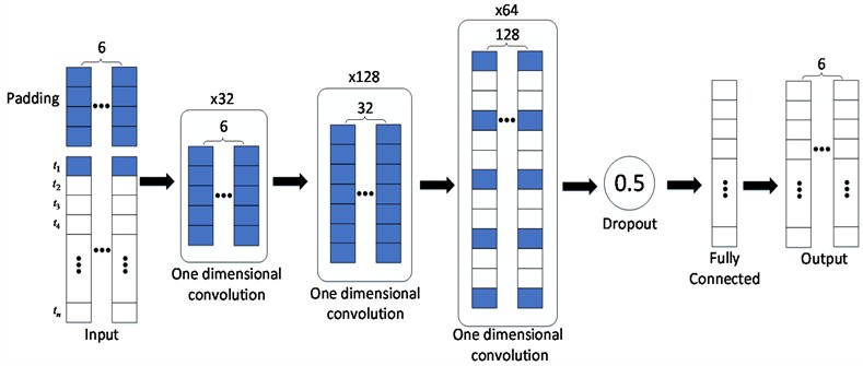
Table 1Process noise CNN structure

Network level	Network name	Content description	Output shape
0	Input	Input layer	( $n$ , 1, 6)
1	Conv1d	Conv1×5	( $n$ , 1, 32)
2	Conv1d	Conv1×7	( $n$ , 1, 128)
3	Conv1d	Conv1×5	( $n$ , 1, 64)
4	Dropout	Dropout (0.5)	( $n$ , 1, 64)
5	Fully connected	Linear(64)	( $n$ , 64)
6	Output	Output layer	( $n$ , 6)

3.3. Adaptive model of CNN observation noise

In the update phase of time n in IEKF, there exists an observation noise covariance matrix $N_{n + 1}$ To adapt to various scenarios, it is necessary to design a noise-adaptive model for the observation noise, allowing the observation noise covariance matrix to adjust adaptively based on different IMU signals. The neural network design of the observation noise adaptive model is illustrated in Fig. 4.

Its input consists of the IMU’s acceleration and angular velocity measurements, while the output is a 2-dimensional vector $z_{n} = [z_{n}^{l a t}, z_{n}^{u p}]$ , which ultimately forms the observation noise covariance matrix $N_{n + 1} \in R^{2 \times 2}$ .The calculation formula is:

20

N_{n + 1} = d i a g (σ_{l a t}^{2} 1 0^{β t a n h (z_{n}^{l a t})}, σ_{u p}^{2} 1 0^{β t a n h (z_{n}^{u p})}),

where $σ_{l a t}^{2}$ and $σ_{u p}^{2}$ represents the initialization parameter of the observation noise covariance. The CNN structure of the observation noise adaptive model is largely consistent with that of the process noise adaptive model, with two primary distinctions: it includes two additional convolutional layers and reduces the number of neurons in the fully connected layer. On the one hand, compared to process noise, observation noise is more closely correlated with IMU measurements. Therefore, a deeper CNN structure with more convolutional filters is designed to extract features more comprehensively and accommodate the dynamic changes in observation noise. On the other hand, given that the parameter count required for modeling the observation noise matrix is lower than that for process noise, the number of neurons in the fully connected layer have reduced to 32 in order to mitigate overfitting. The specific parameters of the observation noise adaptive model's structure are detailed in Table 2.

Fig. 4Observation noise CNN structure

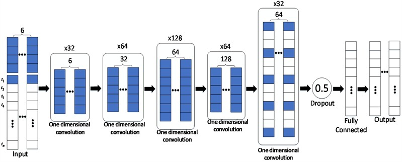
Table 2Observation noise CNN structure

Network level	Network name	Content description	Output shape
0	Input	Input layer	( $n$ , 1, 6)
1	Conv1d	Conv1×5	( $n$ , 1, 32)
2	Conv1d	Conv1×5	( $n$ , 1, 64)
3	Conv1d	Conv1×7	( $n$ , 1, 128)
4	Conv1d	Conv1×5	( $n$ , 1, 64)
5	Conv1d	Conv1×5	( $n$ , 1, 32)
6	Dropout	Dropout(0.5)	( $n$ , 1, 32)
7	Fully connected	Linear(32)	( $n$ , 32)
8	Output	Output layer	( $n$ , 2)

4. Results and analysis

This experiment utilized the large-scale KITTI dataset [26], a widely-used benchmark for autonomous driving algorithms, as the source of test data for the proposed method. For IMU-based vehicle localization, the KITTI dataset provides IMU signals at sampling frequencies of 10 Hz and 100 Hz, collected across various scenarios including urban areas, rural roads, and highways. Given that the 10 Hz data is derived from the original dataset after correcting for camera distortions, this study uses the original 100 Hz dataset to assess the performance of the proposed method.

The proposed method was evaluated on 16 sequences and compared against four other approaches. Among these methods, IEKF represents a filtering method with fixed noise; AI-IMU [29] incorporates a two-layer CNN model to design observation noise within IEKF; CNN [23] employs two distinct CNN models to formulate both process noise and observation noise in IEKF; while CNN-LSTM [23] integrates CNN and LSTM networks to create noise-adaptive models.

4.1. Data processing

The original KITTI dataset contains a substantial amount of video and image. For the purposes of this study, the dataset was cleaned to extract the necessary IMU signal data along with their corresponding ground-truth information. Sequences shorter than 30 seconds were excluded from consideration. The IMU feature data was scaled to ensure similar magnitudes and ranges, eliminating biases caused by scale discrepancies among different features. This preprocessing step enhances the neural network’s ability to effectively extract and learn significant features. The standardization formula is:

21

u_{n o r m a l i z e d} = \frac{u - μ}{σ},

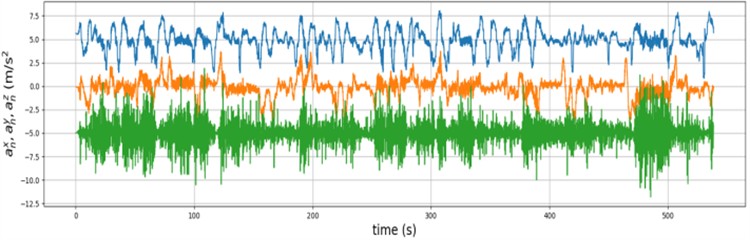
where $u_{n o r m a l i z e d}$ represents the standardized data, $u$ is the original data, $μ$ and $σ$ is the mean and standard deviation of the original data, respectively. The IMU signals before standardization are shown in Fig. 5, where the signals have varying scale ranges.

After standardization, in Fig. 6, a translation operation was applied for better visualization. It can be observed that the components along the three axes are effectively constrained within similar ranges.

Fig. 5Original IMU data

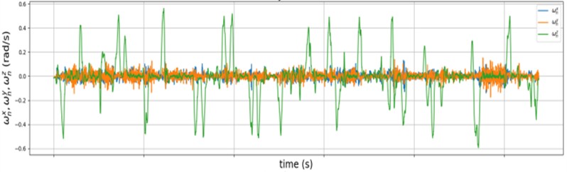
a) Gyrometer

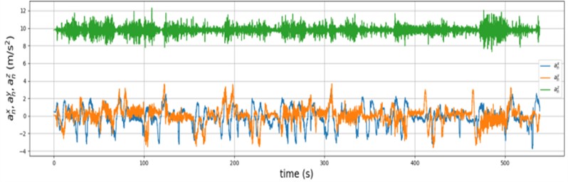
b) Accelerometer

4.2. Error analysis

The evaluation metric of KITTI data set for the accuracy of outdoor automatic driving odometer is the average relative translation error of the predicted trajectory and the real trajectory on the ground in all sub sequences (100 m, 200 m, 300 m, ..., 800 m). The calculation formula is:

22

E_{t r a n s} = \frac{1}{| F |} \sum_{(i, j) \in F}^{} \frac{T r a n s (({\hat{p}}_{j} - {\hat{p}}_{i}) - (p_{j} - p_{i}))}{l e n g t h (i, j)},

where $i$ , $j$ denote the position subscript of the fixed distance, length $(i, j) \in$ (100 m, 200 m, 300 m, …, 800 m) is the distance between them, ${\hat{p}}_{j}$ and $p_{j}$ represent the predicted value and the true value respectively, the $F$ is the whole trajectory set.

Fig. 6Standardized IMU data

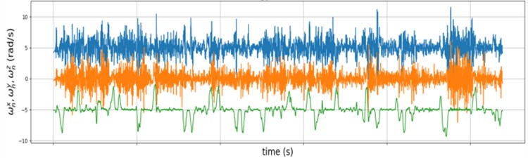
a) Normalized gyro measurements

b) Normalized accelerometer measurements

Table 3 summarized the average relative translation error metrics obtained by various methods across 16 sequences. From the average scores of all sequences, it is evident that all methods reduce the error compared to the IEKF method. Notably, the proposed method achieves the smallest average relative translation error, demonstrating superior localization accuracy. It is important to highlight that while CNN-LSTM outperforms AI-IMU but performs worse than CNN, indicating that CNN models are more effective at dynamically adjusting process and observation noise than LSTM models. Specifically, in sequence 00 and 08, the localization accuracy of AI-IMU, CNN, and CNN-LSTM not only fails to surpass that of pure IEKF but also shows a decline in performance. In contrast, the proposed method continues to reduce error rates, further validating its superiority and ability to provide high-precision localization across diverse scenarios.

Table 3 illustrates the superiority of the proposed method in terms of relative translation error within a specified time range. To further validate the method from various perspectives, additional metrics such as cumulative distribution of errors, root mean square error (RMSE), and absolute position error were analyzed and compared. Fig. 7 presents the cumulative error distribution across different methods. In comparison to the other four methods, the proposed approach demonstrates superior performance in achieving an optimal cumulative error distribution on both the $x$ , $y$ -plane and $z$ -axis. Among the four non-IEKF methods, all are capable of constraining errors within 1.6 meters on the $x$ , $y$ plane. However, along the $z$ -axis, only the proposed methods can limit errors to within 1.6 meters, while the errors of the other methods exceed 1.8 meters. This demonstrates that the CNN structure of the proposed method is well-suited for three-dimensional spatial scenarios.

Table 3Comparison of relative translation errors of different positioning methods

Number	Time(s)	IEKF (%)	AI-IMU (%)	CNN (%)	CNN-LSTM (%)	Proposed (%)
00	45	2.09	2.54	2.32	2.15	1.82
01	32	1.32	1.03	0.96	0.91	0.94
02	48	1.35	0.96	0.94	0.98	0.74
03	80	2.07	1.72	1.51	1.8	1.21
04	80	1.57	1.08	0.93	0.92	0.75
05	44	1.41	1.19	0.8	1.09	0.94
06	57	1.9	1.62	1.56	1.56	1.28
07	42	2.04	1.99	2.09	2.15	1.91
08	48	1.66	2.79	2.12	2.52	1.53
09	28	1.24	1.08	0.72	1.03	0.68
10	111	1.59	1.18	1.18	1.2	1.18
11	111	1.33	0.77	0.71	0.87	0.68
12	518	2.44	2.3	2.16	2.22	2.1
13	160	1.48	1.28	1.13	1.23	0.81
14	123	1.78	1.26	1.33	1.32	1.1
15	117	2.12	1.88	1.85	1.96	1.29
average		2.05	1.83	1.73	1.8	1.56

Fig. 7Comparison of cumulative error distribution

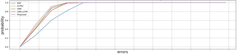
a) On $x y$

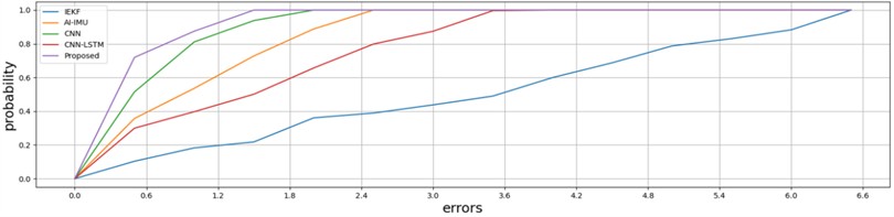
b) On $z$

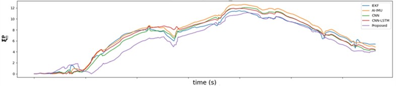
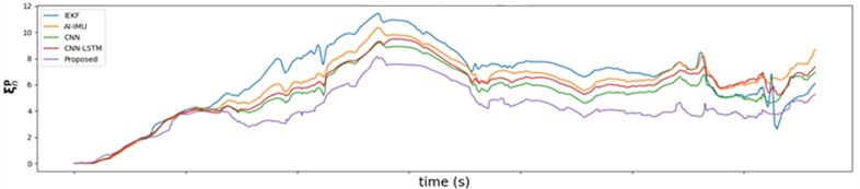
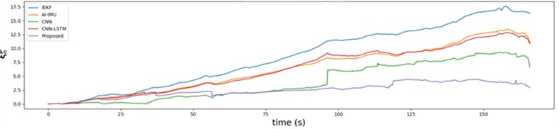
Fig. 8 illustrates the variation of RMSE over time on the $x$ , $y$ -plane and along the $z$ -axis for various methods.

Throughout the entire localization process, the proposed method consistently achieves the lowest RMSE. Although the RMSE of all methods increase over time, the proposed approach effectively mitigates error growth, particularly along the $z$ -axis, where RMSE shows minimal significant increase. The IEKF method exhibits consistently higher RMSE values, with a notable divergence on the $z$ -axis that peaks at 17.5 meters. AI-IMU and CNN-LSTM also show increasing RMSE on the $z$ -axis, with reach maximums of 12.5 meters. In contrast, the proposed method the best RMSE performance, proving the superiority of the dual-noise CNN adaptive model.

The variation of absolute position error over time for different methods are presented in Fig. 9. Across the $x$ , $y$ , $z$ -axes, the proposed method maintains the lowest absolute position error throughout the localization process when compared to the other four methods, remaining in close proximity to the ground truth trajectory. This demonstrates the proposed method’s superior ability to suppress error growth. On the $z$ -axis, the IEKF method demonstrates the highest level of error, while CNN maintains a second-best performance following that of the proposed method.

Fig. 8Comparison of root mean square error

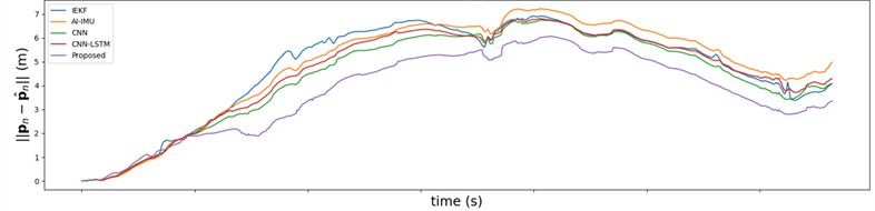
a) On $x y$

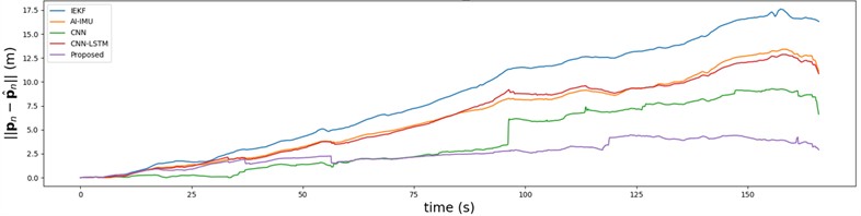
b) On $z$

Fig. 9Comparison of absolute position error

a) On $x$

b) On $y$

c) On $z$

In summary, the proposed method achieves the best localization performance on the $x$ , $y$ plane and the $z$ -axis. CNN come in second, while CNN-LSTM and AI-IMU improve IEKF to some extent.

4.3. Trajectory comparison

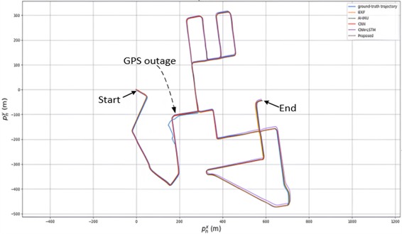
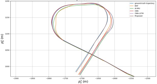
To visually illustrate the performance of the proposed method, Sequence 12, which represents the longest trajectory, was selected for a comprehensive comparison. As depicted in Fig. 10, the total trajectory spans 4.2 km and lasts for 9 minutes. All five methods effectively mitigate errors over this duration. Whether in straight segments, at turning points, or areas where GPS signal loss causes anomalies in the ground-truth trajectory, all methods demonstrate a close alignment with the ground-truth trajectory.

Fig. 10Overall trajectory comparison

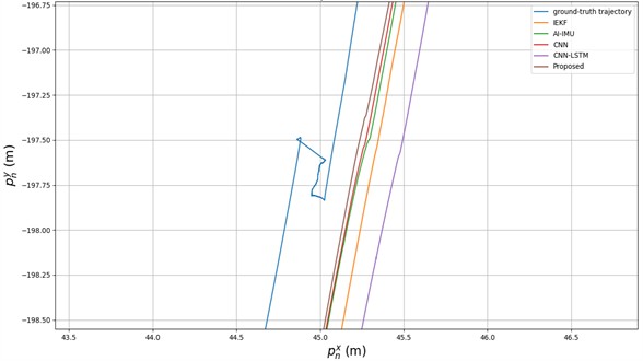
As time progresses, errors gradually accumulate, reaching their peak at the end of the sequence. To better illustrate the performance of the proposed method, a trajectory comparison at the endpoint of the sequence is presented in Fig. 11.

Fig. 11Comparison of trajectories at the end of the sequence

At the end of the sequence, the proposed method demonstrates the best performance compared to the four other methods, remaining the closest to the ground-truth trajectory. This indicates that the proposed method effectively suppresses accumulated errors and trajectory divergence. It is noteworthy that the AI-IMU, CNN, and CNN-LSTM methods perform less favorably than IEKF at the sequence’s endpoint. This suggests that, the other three noise-adaptive methods fail to further improve the error suppression of IEKF over time, whereas the proposed method continues to provide enhancement.

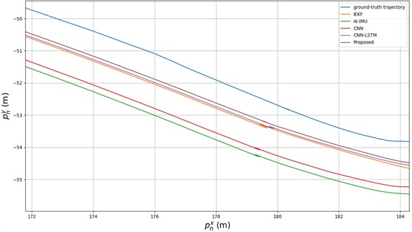
When anomalies occur in the ground-truth trajectory, they may impact the prediction performance of the model. In Fig. 12, despite the presence of anomalies in the ground-truth trajectory, the proposed method remains the closest to the ground truth with minimal error compared to four other methods. In contrast, the localization error associated with CNN-LSTM surpassed that of IEKF, suggesting that an inappropriate neural network model not only fails to mitigate errors but may also reduce localization accuracy.

Fig. 12Comparison of trajectory anomalies in real trajectories

One advantage of inertial localization is the ability to produce smooth localization curves. However, erroneous position estimates during actual localization may lead to discontinuities or unsmooth trajectory phenomena. In Fig. 13, regarding the smoothness of the predicted trajectories, similar unsmooth points appear in the results of the other four methods. Conversely, the proposed method maintains trajectory smoothness and remains closet to the ground truth.

Fig. 13Comparison of smoothness of predicted trajectories

5. Conclusions

To address the rapid error divergence caused by accumulation in pure IMU localization with low- and medium-precision IMUs, this paper proposes a CNN-enhanced adaptive IEKF filtering method, utilizing vehicle localization as the application context. This approach designs deeper one-dimensional CNN models for both process noise and observation noise in IEKF, dynamically adjusting them based on IMU measurement data. An improved convolution technique is introduced to ensure real-time position prediction and reduce errors relative to the ground-truth trajectory. The proposed method was tested and evaluated using the KITTI dataset and its corresponding evaluation metrics. Experimental results demonstrate that: 1) Compared to LSTM models, CNN models are better suited for establishing the relationship between IMU measurements and process/observation noise. 2) When compared to four other pure IMU localization methods, the proposed approach does not rely on any sensors within a specified time range, and further enhances localization accuracy, reduces cumulative errors, produces smoother localization trajectories that are closer to the ground truth.

References

J. Luo, K. Wu, Y. Wang, T. Wang, G. Zhang, and Y. Liu, “An improved UKF for IMU state estimation based on modulation LSTM neural network,” IEEE Transactions on Intelligent Transportation Systems, Vol. 25, No. 9, pp. 10702–10711, Sep. 2024, https://doi.org/10.1109/tits.2024.3368040

Publisher
T. Zhang, M. Yuan, L. Wang, H. Tang, and X. Niu, “A robust and efficient IMU array/GNSS data fusion algorithm,” IEEE Sensors Journal, Vol. 24, No. 16, pp. 26278–26289, Aug. 2024, https://doi.org/10.1109/jsen.2024.3418383

Publisher
R. Kumar Reddy Damagatla and M. Atia, “Improving EKF-based IMU/GNSS fusion using machine learning for IMU denoising,” IEEE Access, Vol. 12, pp. 114358–114369, Jan. 2024, https://doi.org/10.1109/access.2024.3440314

Publisher
J. Gučević, S. Delčev, and O. Vasović Šimšić, “Practical limitations of using the tilt compensation function of the GNSS/IMU receiver,” Remote Sensing, Vol. 16, No. 8, p. 1327, Apr. 2024, https://doi.org/10.3390/rs16081327

Publisher
T. Kim, G. Pak, and E. Kim, “GRIL-Calib: targetless ground robot IMU-LiDAR extrinsic calibration method using ground plane motion constraints,” IEEE Robotics and Automation Letters, Vol. 9, No. 6, pp. 5409–5416, Jun. 2024, https://doi.org/10.1109/lra.2024.3392081

Publisher
T. Okawara et al., “Tightly-coupled LiDAR-IMU-wheel odometry with online calibration of a kinematic model for skid-steering robots,” arXiv:2404.02515, Jan. 2024, https://doi.org/10.48550/arxiv.2404.02515

Publisher
B. van Herbruggen et al., “Strategy analysis of badminton players using deep learning from IMU and UWB wearables,” Internet of Things, Vol. 27, p. 101260, Oct. 2024, https://doi.org/10.1016/j.iot.2024.101260

Publisher
X. Li, S. Chen, S. Li, Y. Zhou, and S. Wang, “Accurate and consistent spatiotemporal calibration for heterogenous-camera/ IMU/LiDAR system based on continuous-time batch estimation,” IEEE/ASME Transactions on Mechatronics, Vol. 29, No. 3, pp. 2009–2020, Jun. 2024, https://doi.org/10.1109/tmech.2023.3323278

Publisher
C. Chen and X. Pan, “Deep learning for inertial positioning: a survey,” IEEE Transactions on Intelligent Transportation Systems, Vol. 25, No. 9, pp. 10506–10523, Sep. 2024, https://doi.org/10.1109/tits.2024.3381161

Publisher
Y. Zhu, J. Zhang, Y. Zhu, B. Zhang, and W. Ma, “RBCN-Net: a data-driven inertial navigation algorithm for pedestrians,” Applied Sciences, Vol. 13, No. 5, p. 2969, Feb. 2023, https://doi.org/10.3390/app13052969

Publisher
J. Brotchie, W. Li, A. D. Greentree, and A. Kealy, “RIOT: recursive inertial odometry transformer for localisation from low-cost IMU measurements,” Sensors, Vol. 23, No. 6, p. 3217, Mar. 2023, https://doi.org/10.3390/s23063217

Publisher
B. Zeinali, H. Zanddizari, and M. J. Chang, “IMUNet: efficient regression architecture for inertial IMU navigation and positioning,” IEEE Transactions on Instrumentation and Measurement, Vol. 73, No. 1, pp. 1–13, Jan. 2024, https://doi.org/10.1109/tim.2024.3381717

Publisher
R. Lai, Y. Tian, J. Tian, J. Wang, N. Li, and Y. Jiang, “ResMixer: a lightweight residual mixer deep inertial odometry for indoor positioning,” IEEE Sensors Journal, Vol. 24, No. 19, pp. 30875–30884, Oct. 2024, https://doi.org/10.1109/jsen.2024.3443311

Publisher
Y. Wang, H. Cheng, and M. Q.-H. Meng, “Spatiotemporal co-attention hybrid neural network for pedestrian localization based on 6D IMU,” IEEE Transactions on Automation Science and Engineering, Vol. 20, No. 1, pp. 636–648, Jan. 2023, https://doi.org/10.1109/tase.2022.3164966

Publisher
B. Rao, E. Kazemi, Y. Ding, D. M. Shila, F. M. Tucker, and L. Wang, “CTIN: robust contextual transformer network for inertial navigation,” in Proceedings of the AAAI Conference on Artificial Intelligence, Vol. 36, No. 5, pp. 5413–5421, Jun. 2022, https://doi.org/10.1609/aaai.v36i5.20479

Publisher
R. K. Jayanth, Y. Xu, Z. Wang, E. Chatzipantazis, D. Gehrig, and K. Daniilidis, “EqNIO: subequivariant neural inertial odometry,” arXiv:2408.06321, Jan. 2024, https://doi.org/10.48550/arxiv.2408.06321

Publisher
L. X. Lin, J. C. Zheng, G. H. Huang, and G. W. Cai, “Utilizing extended Kalman filter to improve convolutional neural networks based monocular visual-inertial odometry,” Chinese Journal of Scientific Instrument, Vol. 42, No. 10, pp. 188–198, 2021, https://doi.org/10.19650/j.cnki.cjsi.j2108267

Publisher
C. Chen, C. X. Lu, B. Wang, N. Trigoni, and A. Markham, “DynaNet: neural Kalman dynamical model for motion estimation and prediction,” IEEE Transactions on Neural Networks and Learning Systems, Vol. 32, No. 12, pp. 5479–5491, Dec. 2021, https://doi.org/10.1109/tnnls.2021.3112460

Publisher
Y. Almalioglu, M. Turan, M. R. U. Saputra, P. P. B. de Gusmão, A. Markham, and N. Trigoni, “SelfVIO: self-supervised deep monocular visual-inertial odometry and depth estimation,” Neural Networks, Vol. 150, pp. 119–136, Jun. 2022, https://doi.org/10.1016/j.neunet.2022.03.005

Publisher
W. Liu et al., “TLIO: tight learned inertial odometry,” IEEE Robotics and Automation Letters, Vol. 5, No. 4, pp. 5653–5660, Oct. 2020, https://doi.org/10.1109/lra.2020.3007421

Publisher
M. Zmitri, H. Fourati, and C. Prieur, “BiLSTM network-based extended Kalman filter for magnetic field gradient aided indoor navigation,” IEEE Sensors Journal, Vol. 22, No. 6, pp. 4781–4789, Mar. 2022, https://doi.org/10.1109/jsen.2021.3091862

Publisher
J. Park, J. Hong Lee, and C. Gook Park, “Pedestrian stride length estimation based on bidirectional LSTM and CNN Architecture,” IEEE Access, Vol. 12, pp. 124718–124728, Jan. 2024, https://doi.org/10.1109/access.2024.3454049

Publisher
W. Dong, “Research on vehicle localization algorithm based on IMU,” China University of Mining and Technology, Beijing, 2021.

Search CrossRef
Z. A. Bature, S. B. Abdullahi, W. Chiracharit, and K. Chamnongthai, “Translated pattern-based eye-writing recognition using dilated causal convolution network,” IEEE Access, Vol. 12, pp. 59079–59092, Jan. 2024, https://doi.org/10.1109/access.2024.3390746

Publisher
H. Wang, B. Bai, J. Li, H. Ke, and W. Xiang, “3D human pose estimation method based on multi-constrained dilated convolutions,” Multimedia Systems, Vol. 30, No. 5, pp. 1–17, Aug. 2024, https://doi.org/10.1007/s00530-024-01441-6

Publisher
J. Wu, S. Huang, Y. Yang, and B. Zhang, “Evaluation of 3D LiDAR SLAM algorithms based on the KITTI dataset,” The Journal of Supercomputing, Vol. 79, No. 14, pp. 15760–15772, Apr. 2023, https://doi.org/10.1007/s11227-023-05267-3

Publisher
B. Or, N. Segol, A. Eweida, and M. Freydin, “Learning position from vehicle vibration using an inertial measurement unit,” IEEE Transactions on Intelligent Transportation Systems, Vol. 25, No. 9, pp. 10766–10776, Sep. 2024, https://doi.org/10.1109/tits.2024.3422037

Publisher
U. Shafiq, A. Waris, J. Iqbal, and S. O. Gilani, “A fusion of EMG and IMU for an augmentative speech detection and recognition system,” IEEE Access, Vol. 12, pp. 14027–14039, Jan. 2024, https://doi.org/10.1109/access.2024.3356597

Publisher
M. Brossard, A. Barrau, and S. Bonnabel, “AI-IMU dead-reckoning,” IEEE Transactions on Intelligent Vehicles, Vol. 5, No. 4, pp. 585–595, Dec. 2020, https://doi.org/10.1109/tiv.2020.2980758

Publisher

About this article

Received

04 January 2025

Accepted

19 March 2025

Published

13 April 2025

SUBJECTS

Vibration in transportation engineering

DOI

https://doi.org/10.21595/jve.2025.24765

Keywords

IMU localization

invariant extended Kalman filter

convolutional neural network

noise adaption

Acknowledgements

The study was supported by the Chongqing Municipal Education Commission's Cooperation Project between Universities in Chongqing and Institutes under the Chinese Academy of Sciences, China (HZ2021009). Chongqing Natural Science Foundation, China (CSTB2024NSCQ-MSX0275). Joint Technical Research Project of Chongqing City Investment Infrastructure Construction Co., Ltd., China (Research on Key Technologies for Safety Control of Mountain Ridge Tunnel Construction in Complex Geological Environments).

Data Availability

The datasets generated during and/or analyzed during the current study are available from the corresponding author on reasonable request.

Author Contributions

J. Han: writing-review and editing, writing-original draft, validation, methodology, investigation, formal analysis, data curation, conceptualization. Z. W. Hou: writing-review and editing, supervision, project administration, methodology, funding acquisition, conceptualization. T. Zhang: resources, funding acquisition. S. X. Wu: experiments, data processing. D. Y. Xu: data curation, formal analysis.

Conflict of interest

The authors declare that they have no conflict of interest.

This is an open access article distributed under the Creative Commons Attribution License, which permits unrestricted use, distribution, and reproduction in any medium, provided the original work is properly cited.

Research article

2023 11 18

Vehicle state and parameter estimation based on adaptive anti-outlier unscented Kalman filter and GA-BPNN method

Yingjie Liu, Dawei Cui, Wen Peng

Research article

2023 10 30

Vehicle state and parameter estimation based on improved extend Kalman filter

Yingjie Liu, Dawei Cui, Wen Peng

Research article

2020 08 15

Bearing fault diagnosis based on improved VMD and DCNN

Ran Wang, Lei Xu, Fengkai Liu

Research article

2018 11 15

Bearing fault feature extraction method based on complete ensemble empirical mode decomposition with adaptive noise

Maohua Xiao, Cunyi Zhang, Kai Wen, Longfei Xiong, Guosheng Geng, Dan Wu

J. Han, Z. W. Hou, T. Zhang, S. X. Wu, and D. Y. Xu, “Pure IMU localization for intelligent platforms with CNN adaptive invariant extended Kalman filter noise fusion,” Journal of Vibroengineering, Vol. 27, No. 4, –17, Apr. 2025, https://doi.org/10.21595/jve.2025.24765

Copy Extrica

Copied to clipboard!

TY  - JOUR
DO  - 10.21595/jve.2025.24765
UR  - https://doi.org/10.21595/jve.2025.24765
TI  - Pure IMU localization for intelligent platforms with CNN adaptive invariant extended Kalman filter noise fusion
T2  - Journal of Vibroengineering
AU  - Han, J.
AU  - Hou, Z. W.
AU  - Zhang, T.
AU  - Wu, S. X.
AU  - Xu, D. Y.
PY  - 2025
DA  - 2025/04/13
PB  - Extrica
VL  - 27
IS  - 4
SN  - 1392-8716
SN  - 2538-8460
ER  - 

Copy Ris

Copied to clipboard!

 @article{Han_2025, title={Pure IMU localization for intelligent platforms with CNN adaptive invariant extended Kalman filter noise fusion}, ISSN={2538-8460}, url={https://doi.org/10.21595/jve.2025.24765}, DOI={10.21595/jve.2025.24765}, journal={Journal of Vibroengineering}, publisher={JVE International Ltd.}, author={Han, J. and Hou, Z. W. and Zhang, T. and Wu, S. X. and Xu, D. Y.}, year={2025}, month=apr }

Copy Bibtex

Copied to clipboard!

[1]J. Han, Z. W. Hou, T. Zhang, S. X. Wu, and D. Y. Xu, “Pure IMU localization for intelligent platforms with CNN adaptive invariant extended Kalman filter noise fusion,” Journal of Vibroengineering, Apr. 2025, doi: 10.21595/jve.2025.24765.

Copy IEEE

Copied to clipboard!

Han, J., Z. W. Hou, T. Zhang, S. X. Wu, and D. Y. Xu. “Pure IMU Localization for Intelligent Platforms with CNN Adaptive Invariant Extended Kalman Filter Noise Fusion.” Journal of Vibroengineering, April 13, 2025. https://doi.org/10.21595/jve.2025.24765.

Copy Chicago

Copied to clipboard!

Pure IMU localization for intelligent platforms with CNN adaptive invariant extended Kalman filter noise fusion

Abstract

Highlights

1. Introduction

2. Pure IMU modeling and localization

2.1. IMU modeling

2.2. Localization modeling

3. Noise adaptive IMU filtering method based on CNN

3.1. IEKF principle

3.1.1. State transition equation

3.1.2. Observation equation

3.1.3. IEKF update steps

3.2. Adaptive model of CNN process noise

3.3. Adaptive model of CNN observation noise

4. Results and analysis

4.1. Data processing

4.2. Error analysis

4.3. Trajectory comparison

5. Conclusions

References

About this article

Related Articles