DC charging pile energy measurement method based on wavelet threshold denoising and smoothing optimization

Jiaying, Li; Gang, Qin; Xian, Yang; Danqing, Luo; Jue, Huang; Yunpeng, Gao

doi:10.21595/jme.2026.25074

Journal of Measurements in Engineering

Browse Journal

Submit article

Published: October 31, 2026

Check for updates

DC charging pile energy measurement method based on wavelet threshold denoising and smoothing optimization

Li Jiaying¹

Qin Gang²

Yang Xian³

Luo Danqing⁴

Huang Jue⁵

Gao Yunpeng⁶

^{1, 2, 3, 4, 5, 6}Hainan Power Grid Co. Ltd., Hainan, 570203, China

Corresponding Author:

Li Jiaying

Cite the article Download PDF

Article in Press

Downloads 0

Abstract

In the context of DC charging for electric vehicles, noise interference in DC grid signals significantly compromises the accuracy of energy measurement during charging, leading to potential billing inaccuracies and operational inefficiencies. To address this challenge, this paper proposes a high-precision energy measurement method for DC charging piles, integrating wavelet threshold denoising and signal smoothing techniques. First, an improved wavelet threshold denoising algorithm is applied to process the noisy raw signals. Unlike conventional approaches, this method employs particle swarm optimization (PSO) to dynamically determine the optimal parameters of a soft-hard threshold compromise function, ensuring near-optimal noise suppression while preserving critical signal features. Following denoising, a moving average smoothing filter is applied to further refine the signal, reducing residual fluctuations. The final energy measurement is computed using gradient integration, enhancing precision in cumulative energy calculations. Addressing the noise and precision challenges in DC charging pile metering requires a dedicated signal processing strategy. This work presents an integrated solution combining PSO-based adaptive wavelet denoising with post-processing smoothing to meet these requirements. Simulation experiments demonstrate that the PSO-optimized wavelet denoising algorithm significantly outperforms traditional methods in terms of signal-to-noise ratio and mean squared error, confirming its effectiveness in noise reduction. Additionally, the smoothing process is shown to improve energy measurement accuracy by minimizing transient distortions. A comparative analysis reveals that while cubic spline interpolation offers minor improvements, its impact on overall measurement precision is limited compared to the proposed de-noising-smoothing framework. The proposed method not only enhances the reliability of DC charging energy metering but also provides a robust solution for noise-laden industrial signal processing. Future work will explore real-time implementation and hardware optimization for large-scale charging infrastructure.

1. Introduction

With the rapid development of the new energy vehicle industry, DC charging piles have become essential facilities for electric vehicle charging. The accuracy of their energy measurement is increasingly critical [1]. As nonlinear loads, charging piles produce DC-side signals containing harmonics, noise, and voltage and current fluctuations [2]. These factors not only cause energy measurement errors but also negatively impact the economic interests of both charging users and electricity sellers. Against this backdrop, improving the accuracy of energy measurement for DC charging piles has become a key focus of academic and industrial research.

Currently, researchers have proposed various denoising methods to address noise interference in energy measurement for charging piles. For example, low-pass filters have been used for harmonic suppression, effectively filtering high-frequency noise in power grid signals, but their performance in signal recovery accuracy remains insufficient [3-4]. Median filtering, known for its robustness against impulse noise, is often employed for signal preprocessing but may result in the loss of some useful information [5]. Additionally, power spectral analysis combined with adaptive filters allows for dynamic adjustment of filtering parameters, but the high complexity of the algo-rithm limits its wide application in practical scenarios [6].

In the field of wavelet analysis, wavelet threshold denoising methods have been widely used in energy measurement signal processing due to their advantages in time-frequency domain decomposition. Traditional hard and soft threshold methods have been shown to suppress high-frequency noise to some extent, but their draw-backs include oscillations or fixed biases during signal reconstruction [7]. In recent years, researchers have proposed improved threshold functions, such as adaptive wavelet thresholds and wavelet thresholds optimized by genetic algorithms, to enhance denoising performance. However, these methods still fail to fully address the issue of signal detail loss [8-10]. To improve the accuracy of energy measurement, re-searchers have proposed various dynamic measurement algorithms. For instance, harmonic analysis methods based on wavelet packet decomposition can separate harmonic and interharmonic components in power grid signals. Instantaneous energy analysis methods combined with Hilbert transform have been applied to dynamic energy measurement, but their robustness in high-noise environments remains limited [11]. Additionally, error correction methods based on piecewise linear fitting per-form well for low-frequency signals but are less effective when dealing with complex multi-frequency mixed signals [12]. Traditional hard thresholding suffers from discontinuities that may cause oscillations, while soft thresholding introduces fixed bias. The improved soft-hard threshold compromise function avoids these issues, balancing noise reduction and signal preservation. Its purpose is to combine the strengths of hard and soft thresholds, avoiding oscillations and bias simultaneously, thus enhancing denoising performance.

Although the above studies have improved energy measurement accuracy to some extent, there are still significant shortcomings in terms of denoising quality, signal smoothness, and real-time performance in practical engineering applications. To address these issues, this paper proposes an energy measurement method that com-bines improved wavelet threshold denoising with the moving average method. By introducing particle swarm optimization (PSO) to determine the denoising parameters, the method achieves near-optimal denoising. The moving average method is then ap-plied to further enhance signal smoothness, significantly improving energy measure-ment accuracy. This approach integrates advanced denoising techniques with optimization algorithms, providing a new solution and practical foundation for high-accuracy energy measurement in DC charging piles. The principal novelty of this work is threefold: (1) the introduction of a Particle Swarm Optimization (PSO) framework to dynamically determine the optimal parameters ( $k_{1}$ and $k_{2}$ ) of an improved soft-hard threshold compromise wavelet function, moving beyond fixed or empirically set parameters; (2) the structured two-stage signal enhancement process that sequentially applies this optimized denoising followed by a moving average smoothing filter, specifically designed to minimize residual fluctuations critical for accurate energy integration; and (3) the holistic application of this combined denoising-smoothing-optimization framework to the specific problem of DC charging pile energy measurement, demonstrating superior performance over conventional and alternative advanced methods.

2. DC energy measurement method

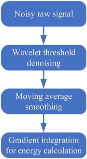
The flowchart of the proposed DC energy metering method is shown in Fig. 1. For the noisy raw signals on the DC side, wavelet denoising and smoothing processes are applied, followed by the use of the gradient integration method to calculate the DC energy. In practical scenarios, the DC grid signals contain noise, voltage fluctuations, current fluctuations, etc., which can affect the calculation results. To address the noise in the DC grid signals, the paper introduces a wavelet threshold denoising algorithm to filter out the noise in the voltage and current signals as much as possible, thus im-proving the accuracy of the calculation results.

Fig. 1Signal processing flow

3. Wavelet threshold denoising algorithm

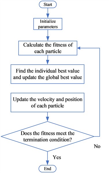
After wavelet decomposition of the DC grid signal, the energy of low-order harmonic signals is concentrated in the low-frequency coefficients, while the noise energy and a small amount of high-order harmonics are distributed in the high-frequency coefficients. Therefore, it is necessary to set an appropriate threshold based on the characteristics of the wavelet transform. The wavelet coefficients outside the threshold range are retained, and those within the threshold range are removed, thus achieving signal denoising. The flowchart of the wavelet threshold denoising algorithm based on particle swarm optimization for parameter setting is shown in Fig. 2.

Fig. 2Multi-scale feature extraction module structure

3.1. Wavelet threshold function

The traditional wavelet threshold functions include the hard threshold function and the soft threshold function [13-14]. The expression of the hard threshold function is shown in Eq. (1), and the expression of the soft threshold function is shown in Eq. (2):

1

{\hat{ω}}_{j, k} = \{\begin{array}{l} ω_{j, k}, |ω_{j, k}| \geq λ, \\ 0, |ω_{j, k}| < λ, \end{array}

2

{\hat{ω}}_{j, k} = \{\begin{array}{l} sgn (ω_{j, k}) (|ω_{j, k}| - λ), |ω_{j, k}| \geq λ, \\ 0, |ω_{j, k}| < λ, \end{array}

where, $ω_{j, k}$ is the $k$ -th coefficient in the detail coefficient array of the $j$ -th level after wavelet decomposition of the noisy signal. ${\hat{ω}}_{j, k}$ is the estimated wavelet coefficient after processing by the threshold function. $λ$ is the threshold value, and $s g n (x)$ is the sign function.

The hard threshold function contains discontinuities, which can cause oscillations in the reconstructed signal [15]. Although the soft threshold function does not have discontinuities, a fixed bias exists between $ω_{j, k}$ and ${\hat{ω}}_{j, k}$ when $|ω_{j, k}| \geq λ$ . This bias is unfavorable for separating useful signals from noise. To address the shortcomings of both hard and soft threshold functions, researchers have proposed an improved wavelet threshold function – the improved soft-hard threshold compromise function . The expression of the improved soft-hard threshold compromise function is shown in Eq. (3) [16]. This function aims to combine the strengths of hard and soft thresholds, thereby avoiding oscillations and bias simultaneously and enhancing denoising performance:

3

{\hat{ω}}_{j, k} = \{\begin{array}{l} sgn (ω_{j, k}) (|ω_{j, k}| - λ^{*} (1 - k_{2})), |ω_{j, k}| \geq λ, \\ sgn (ω_{j, k}) |ω_{j, k}| * \frac{{|ω_{j, k}|}^{k_{1}}}{λ^{k_{1}} - 1} * k_{2}, |ω_{j, k}| < λ, \end{array}

where, $k_{1}$ and $k_{2}$ are adjustment factors for the improved threshold function. Here, $k_{1}$ is a constant, and 0 $< k_{2} <$ 1.

The improved soft-hard threshold compromise function has no discontinuities and does not suffer from the fixed bias problem. It addresses the shortcomings of both the hard threshold and soft threshold functions while retaining their respective advantages. This function aims to combine the strengths of hard and soft thresholds, avoiding oscillations and bias simultaneously, thus enhancing denoising performance.

3.2. Threshold of the wavelet threshold function

The traditional wavelet threshold selection rules include the following four types [17]:

1) Universal threshold rule (sqtwolog), with the formula as follows:

4

T = σ \sqrt{2 ln N},

where, $σ$ is the noise standard deviation, and $N$ is the signal length.

2) Unbiased risk estimate rule (rigrsure). It is derived from the soft threshold function and based on the principle of unbiased estimation of mean squared error.

3) Heuristic unbiased risk estimate rule (heursure). It is a compromise between rule 1) and rule 2).

4) Minimax rule (minimaxi). Its principle is to perform Bayesian estimation using prior information of the true wavelet coefficients.

Among the above threshold selection rules, rule 2) and rule 4) can retain weak useful signals and are suitable for cases where noise is less distributed in the high-frequency components of the signal. In contrast, rule 1) and rule 3) may misjudge high-frequency signals as noise. Another type of layered threshold decreases as the number of wavelet decomposition levels increases, which is consistent with the variation pattern of noise wavelet coefficients. This layered threshold reduces bias and improves the accuracy of the threshold. The calculation expression of the layered threshold is shown in Eq. (5):

5

λ_{j} = \frac{σ \sqrt{2 ln (N)}}{\ln (j + 1)},

where, $σ$ represents the estimated standard deviation of the noise, $N$ denotes the length of the wavelet coefficients after decomposition, $j$ indicates the wavelet decomposition level, and $λ_{j}$ represents the threshold for the $j$ -th decomposition level.

3.3. Parameter determination of the wavelet threshold function

The wavelet threshold function mentioned above contains two parameters, $k_{1}$ and $k_{2}$ , whose selection directly impacts the effectiveness of wavelet threshold denoising. This problem can be abstracted as an optimization problem, where the goal is to calculate the approximate optimal values of $k_{1}$ and $k_{2}$ through an algorithm to achieve near-optimal denoising performance. In this paper, particle swarm optimization is used to determine the approximate optimal values of $k_{1}$ and $k_{2}$ , and the algorithm flowchart is shown in Fig 3.

Fig. 3Particle swarm optimization process

The output signal-to-noise ratio (SNR) and the output signal root mean square error (RMSE) are selected as the indicators for measuring the wavelet threshold denoising performance. The formulas for calculating these two indicators are shown in Eqs. (6) and (7):

6

S N R = 10 l g (\frac{\sum_{n = 1}^{N} s^{2} (n)}{\sum_{n = 1}^{N} [s^{2} (n) - {\hat{s}}^{2} (n)]}),

7

R M S E = \sqrt{\frac{1}{N} \sum_{n = 1}^{N} [s^{2} (n) - {\hat{s}}^{2} (n)]},

where, $s (n)$ is the noisy original signal, and $\hat{s} (n)$ is the denoised signal. The larger the value of SNR and the smaller the value of RMSE, the better the performance of wavelet threshold denoising.

PSO was selected over genetic algorithms and simulated annealing because of its simpler implementation, faster convergence, and robustness in low-dimensional optimization problems, which better satisfy real-time requirements.

Therefore, the fitness function in the particle swarm algorithm can be constructed as shown in Eq. (8):

8

f = \frac{1}{S N R_{1}} + R M S E_{1} + \frac{1}{S N R_{2}} + R M S E_{2},

where, $f$ is the fitness value, SNR₁ and RMSE₂ are the signal-to-noise ratio and root mean square error of the voltage output signal, while SNR₂ and RMSE₂ are the signal-to-noise ratio and root mean square error of the current output signal.

4. Smoothed denoised power grid signal

4.1. Moving average method

The moving average method introduces the concept of a “window”, which slides over the noisy power grid signal. Each time the window slides over an element, the arithmetic mean of the data within the window is calculated. The data within the window is also updated as the window moves [18-19]. Through this process, abrupt elements in the power grid signal are partially eliminated, achieving the goal of smoothing. This step reduces residual fluctuations after denoising, ensuring smoother signals before gradient integration, thereby directly improving energy measurement accuracy.

For the simple smoothing method, there is only one parameter, the window length. Let the window length be $m$ , and the smoothing coefficient is always 1/ $m$ . Let the original signal be $x_{k}$ , where $k =$ 1, 2,…, $n$ . Then, the sliding average formula for the $k$ -th data point is:

9

r_{k} = \frac{1}{m} \sum_{i = k - \frac{m - 1}{2}}^{k + \frac{m - 1}{2}} x_{i},

where, $k \in (\frac{m + 1}{2}, n - \frac{m - 1}{2})$ , where $n$ is the length of the data points.

The window length and smoothing coefficient of the simple smoothing method are fixed values, which are not conducive to effectively smoothing noisy power grid signal data and have poor universality. The MATLAB toolbox provides a smoothing function called smoothdata, which determines the window length in an adaptive manner and returns the moving average of the vector elements, resulting in better smoothing performance.

After the power grid signal is denoised using the wavelet threshold method, it can be smoothed using the moving average method. The power of the power grid signal during DC charging can then be calculated using Eq. (10):

10

W = \sum_{k = 0}^{N - 1} u (t_{k}) i (t_{k}) Δ t,

where, $u (t_{k})$ is the instantaneous voltage, $i (t_{k})$ is the instantaneous current, and $Δ t$ is the time difference between sampling points $t_{k}$ . When $Δ t$ is sufficiently small, the calculated value of this equation is almost equal to the integral of power over time, which represents the energy value. Essentially, this equation is the calculation formula for integration in practical engineering.

If the data quantity of the power grid signal is increased through interpolation methods, it is theoretically possible to further improve the accuracy of DC charging energy measurement.

4.2. Cubic spline interpolation method

In the data processing process, when the data volume is insufficient, interpolation methods can be used to supplement the data points. Cubic spline interpolation is an algebraic interpolation method, which also includes methods such as Lagrange interpolation and Newton interpolation. Compared to Lagrange interpolation and Newton interpolation, cubic spline interpolation eliminates the Runge phenomenon found in Lagrange interpolation and improves the smoothness of Newton interpolation at the nodes. Cubic spline interpolation is a piecewise interpolation method, and the process is as follows.

Divide the given interval $[a, b]$ into several smaller intervals: $a = x_{0} < x_{1} < \dots < x_{n} = b$ . Given that $f (x_{j}) = y_{j}$ , $j = 0,1, \dots, n$ . If:

11

S (x) = \{\begin{array}{l} S_{1} (x), x \in [x_{0}, x_{1}], \\ S_{2} (x), x \in [x_{1}, x_{2}], \\ \dots \\ S_{n} (x), x \in [x_{n - 1}, x_{n}] . \end{array}

Satisfies:

1) $S (x)$ is a cubic polynomial on the interval $[x_{j}, x_{j + 1}]$ .

2) $S^{''} (x)$ is continuous on the interval $[a, b]$ .

3) $S (x_{j}) = y_{j}$ , $j = 0,1, \dots, n$ .

Then, $S (x)$ is called the cubic spline interpolation function. When $x \in [x_{j}, x_{j + 1}]$ , $j = 0,1, \dots, n - 1$ :

12

S_{j} (x) = a_{j} + b_{j} x + c_{j} x^{2} + d_{j} x^{3} .

There are $n$ cubic polynomials, and the number of unknown coefficients is 4 $n$ . To solve for these unknown coefficients, a system of solvable equations needs to be established based on the known conditions, which include interpolation conditions, continuity conditions, and natural boundary conditions. The following equation shows how these conditions can be used to establish 4 $n$ equations.

1) Interpolation condition: $S (x_{i}) = y_{i}$ , $j = 0,1, \dots, n$ .

2) Natural boundary condition: $S^{''} (x_{0}) = 0$ , $S^{''} (x_{n}) = 0$ .

3) Continuity condition:

\{\begin{array}{l} S (x_{j} + 0) = S (x_{j} - 0), \\ S^{'} (x_{j} + 0) = S^{'} (x_{j} - 0), \\ S^{''} (x_{j} + 0) = S^{''} (x_{j} - 0), \\ j = 1,2, \dots, n - 1 . \end{array}

5. Experimental results and analysis

Besides traditional methods, we considered cubic spline interpolation and adaptive filtering methods. Results indicate the proposed denoising-smoothing method achieves superior accuracy.

5.1. Signal model establishment

In the scenario of DC charging at electric vehicle charging stations, the DC grid signal on the DC side contains, in addition to the DC component, the 11th, 13th, and 15th harmonic waves, which have the most significant impact during electric vehicle charging. The harmonic contents are 5 %, 3 %, and 1 %, respectively.

The expression for the original voltage signal u is given in Eq. (13), and the expression for the original current signal $i$ is given in Eq. (14):

13

u (t) = u + 0.05 \sqrt{2} u cos (2 π n_{1} f t) + 0.03 \sqrt{2} u cos (2 π n_{2} f t + 4 π / 5)

+ 0.01 \sqrt{2} u cos (2 π n_{3} f t + \frac{π}{3}),

14

i (t) = i + 0.05 \cdot \sqrt{2} i cos (2 π n_{1} f t + π / 2) + 0.03 \cdot \sqrt{2} i cos (2 π n_{2} f t + π / 3)

+ 0.01 \cdot \sqrt{2} i cos (2 π n_{3} f t + \frac{3 π}{4}),

where, the DC voltage signal $u =$ 500V, the DC current signal $i =$ 60, the fundamental frequency $f =$ 50 $H$ , the harmonic orders are $n_{1} =$ 11, $n_{2} =$ 13, $n_{3} =$ 15, the sampling rate is 100 kHz, and the total simulation time is 0.1 s.

Fig. 4DC energy measurement method

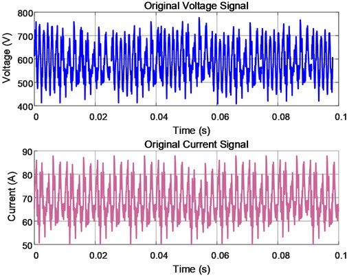
In the scenario of DC charging at electric vehicle charging stations, the voltage and current signals on the DC side contain not only high-order harmonics but also noise. Therefore, Gaussian noise with a SNR of 25 dB is added to the DC side signals containing harmonics in the simulation. The waveforms of the noisy voltage and current signals are shown in Fig. 4.

5.2. Particle swarm optimization algorithm to determine the parameters of the wavelet threshold function

Before applying the wavelet threshold denoising algorithm, the two parameters $k_{1}$ and $k_{2}$ in the improved soft-hard threshold compromise function need to be determined using the particle swarm optimization algorithm. The population size of particles is set to 100, with two parameters as independent variables, so the particle dimension is set to 2. The maximum number of iterations is 400, and the learning factors are $c_{1} =$ 1.5 and $c_{2} =$ 1.5. The inertia weight range is [0.4, 0.8], the position range is [0, 6], and the velocity range is [–1, 1]. The fitness function is shown in Eq. (8). $k_{1}$ converges to approximately 3.507, and $k_{2}$ converges to approximately 0.0978. This function aims to combine the strengths of hard and soft thresholds, avoiding oscillations and bias simultaneously, thus enhancing denoising performance.

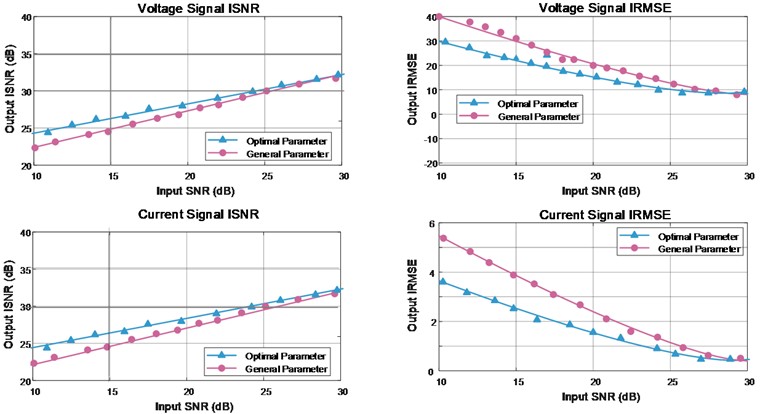
To verify that the approximate optimal parameter values ( $k_{1} =$ 3.507 and $k_{2} =$ 0.0978), determined by the particle swarm optimization algorithm, improve the denoising effect of the wavelet threshold denoising method, a set of typical parameters $k_{1} =$ 6.0 and $k_{2} =$ 0.5 is used as a comparison. The SNR and RMSE of the output signal are calculated for input signals with different signal-to-noise ratios. The results are shown in Fig. 5. As seen from Fig. 5, the parameters determined by the particle swarm optimization algorithm can optimize the denoising effect of the wavelet threshold denoising algorithm.

Fig. 5Comparison of denoising effects between general parameters and approximate optimal parameters

5.3. The results of wavelet threshold denoising

In this paper, an improved soft-hard threshold compromise function and hierarchical threshold are used to construct a wavelet threshold denoising algorithm for noise in the DC-side power grid signal. The wavelet basis is selected as db8, with the wavelet decomposition level set to 6, and $k_{1} =$ 3.507, $k_{2} =$ 0.0978. The SNR of the input noisy original signal is set to 25 dB. The input power grid signal is denoised using the discrete wavelet function, and the output signal's SNR and RMSE are calculated. These two metrics are used to evaluate the denoising performance. This function aims to combine the strengths of hard and soft thresholds, avoiding oscillations and bias simultaneously, thus enhancing denoising performance. Specifically, Daubechies 8 (db8) was used as the wavelet basis, with decomposition level set to 6.

As shown in Figs. 6 and 7, the voltage and current signals are subjected to wavelet threshold denoising using both traditional thresholds and hierarchical thresholds under different input signal-to-noise ratios. The calculated output signal SNR and RMSE are presented. From Figs. 6 and 7, it can be observed that as the input signal SNR increases, the output signal SNR after hierarchical threshold processing remains at a relatively high level, while the RMSE between the output signal and the original signal remains at a low level. Therefore, the wavelet threshold denoising with hierarchical threshold significantly outperforms other traditional thresholds.

Fig. 6Denoising effect of voltage signal under different thresholds

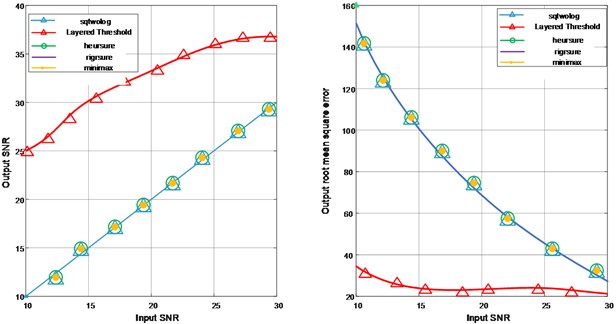
Fig. 7Denoising effect of current signal under different thresholds

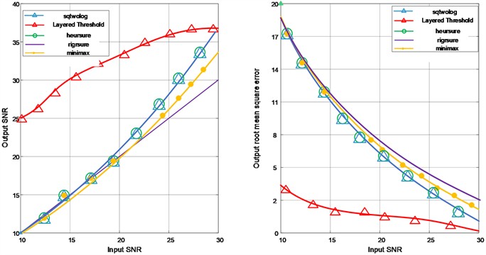
Table 1 calculates the average SNR and average RMSE values for the voltage and current signals, further demonstrating that the wavelet threshold denoising with hierarchical threshold performs better.

Table 1Experimental results

Harmonic extraction method	SNR (Voltage signal)	RMSE (Voltage signal)	SNR (Current signal)	MSE (Current signal)
Layered threshold	32.4	13.30	32.6	1.6
heursure	20.1	63.1	21.2	7.2
Minimaxi	20.1	63.1	20.5	7.5
rigrsure	20.1	63.1	20.1	7.6
sqtwolog	20.1	63.0	21.5	7.2

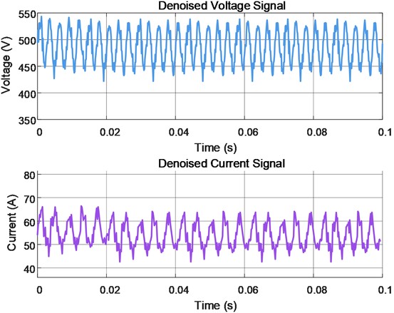
The output signal waveform after denoising the input signal using the hierarchical threshold wavelet threshold denoising algorithm is shown in Fig. 8. It is evident that the denoised signal in Fig. 8 contains significantly less noise compared to the noisy original waveform in Fig. 4.

Fig. 8Denoised signal

5.4. Energy metering after smoothing processing

Direct gradient integration on noisy signals produces large errors. Our approach with denoising and smoothing lowers error variance significantly, as demonstrated in Fig. 9. After wavelet threshold denoising, the noise content in the DC side grid signal is already at a low level. However, as shown in Fig. 8, the denoised signal is still not smooth enough, which may affect the accuracy of the energy metering results. Therefore, the signal after denoising is smoothed using the moving average method, and cubic spline interpolation is applied to the smoothed signal to further improve the accuracy of energy metering.

Fig. 9Electric energy measurement results

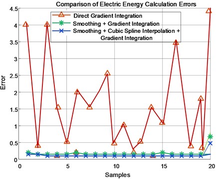
By performing integration on Eq. (13) and (14), the true value of the energy is obtained, which facilitates the calculation of the energy metering error of the method described in the paper in MATLAB simulation. As shown in Fig 9, to improve the reliability of the experimental results, 20 simulations of energy metering were performed in MATLAB. From Fig. 9, it can be observed that directly performing gradient integration on the denoised signal leads to relatively large errors and significant error fluctuations. In contrast, after smoothing the denoised signal using the moving average method and then performing gradient integration, the energy metering error remains consistently low and stable. For the denoised signal, when smoothing is applied followed by cubic spline interpolation and then gradient integration, the energy metering error shows minimal improvement while increasing computational complexity.

6. Conclusions

In this paper, a method combining wavelet threshold denoising and the moving average method is proposed to address the energy metering issue of the DC side in electric vehicle charging piles in DC charging scenarios. The method uses an improved soft-hard threshold compromise function as the wavelet threshold function and selects a hierarchical threshold. Its innovation primarily resides in the PSO-optimized adaptive wavelet denoising coupled with post-denoising signal smoothing. The parameters of the improved soft-hard threshold compromise function are determined using particle swarm optimization. After wavelet threshold denoising of the DC side signal, the signal is further processed using the moving average method to make it smoother, and energy is finally calculated using gradient integration. The paper simulates the DC side grid signal of the electric vehicle charging pile in a DC charging scenario and conducts energy metering experiments. The experimental results show that the denoising effect obtained using the improved soft-hard threshold compromise function with the hierarchical threshold is better than that of traditional thresholds, and the use of particle swarm optimization to determine the approximately optimal parameter values ensures nearly optimal denoising performance. At the same time, the experimental results demonstrate that the moving average method improves the accuracy of energy metering through signal smoothing. However, performing cubic spline interpolation after smoothing does not further enhance energy metering accuracy; this is likely because the smoothing process has already filtered out the high-frequency noise that interpolation could otherwise have misinterpreted as meaningful signal. In future work, we plan to conduct on-site data validation with real charging piles, explore hardware acceleration for real-time implementation, and expand applications to other smart grid scenarios.

References

S. Su, “Method of location and capacity determination of intelligent charging pile based on recurrent neural network,” World Electric Vehicle Journal, Vol. 13, No. 10, p. 186, Oct. 2022, https://doi.org/10.3390/wevj13100186

Publisher
J. Wang, J. Deng, Y. Liu, and Y. Wang, “Non-intrusive load perception and flexibility evaluation for electric vehicle charging station: a deep learning based approach,” in IEEE 5th International Electrical and Energy Conference (CIEEC), pp. 2570–2575, May 2022, https://doi.org/10.1109/cieec54735.2022.9845884

Publisher
“Notice of the state council on printing and distributing the action plan for carbon peaking before 2030,” Gazette of the State Council of the People’s Republic of China, Beijing, China, 2021.

Search CrossRef
S. Lu, X. Feng, G. Lin, J. Wang, and Q. Xu, “Non-intrusive load monitoring and controllability evaluation of electric vehicle charging stations based on K-means clustering optimization deep learning,” World Electric Vehicle Journal, Vol. 13, No. 11, p. 198, Oct. 2022, https://doi.org/10.3390/wevj13110198

Publisher
M. Ebrahimi, M. Rastegar, and M. M. Arefi, “Real-time estimation frameworks for feeder-level load disaggregation and PEVs’ charging behavior characteristics extraction,” IEEE Transactions on Industrial Informatics, Vol. 18, No. 7, pp. 4715–4724, Jul. 2022, https://doi.org/10.1109/tii.2021.3118101

Publisher
P. Zhang, J. Chen, L. Tu, and L. Yin, “Layout evaluation of new energy vehicle charging stations: a perspective using the complex network robustness theory,” World Electric Vehicle Journal, Vol. 13, No. 7, p. 127, Jul. 2022, https://doi.org/10.3390/wevj13070127

Publisher
S. Liu et al., “Non-invasive load decomposition method based on multi-feature objective function PCA-ILP,” Electric Power Construction, Vol. 41, 2020.

Search CrossRef
A. Faustine and L. Pereira, “Multi-label learning for appliance recognition in NILM using fryze-current decomposition and convolutional neural network,” Energies, Vol. 13, No. 16, p. 4154, Aug. 2020, https://doi.org/10.3390/en13164154

Publisher
R. V. A. Monteiro, J. C. R. de Santana, R. F. S. Teixeira, A. S. Bretas, R. Aguiar, and C. E. P. Poma, “Non-intrusive load monitoring using artificial intelligence classifiers: Performance analysis of machine learning techniques,” Electric Power Systems Research, Vol. 198, p. 107347, Sep. 2021, https://doi.org/10.1016/j.epsr.2021.107347

Publisher
F. Ciancetta, G. Bucci, E. Fiorucci, S. Mari, and A. Fioravanti, “A new convolutional neural network-based system for NILM applications,” IEEE Transactions on Instrumentation and Measurement, Vol. 70, pp. 1–12, Jan. 2021, https://doi.org/10.1109/tim.2020.3035193

Publisher
A. Mirzal, “Statistical analysis of microarray data clustering using NMF, spectral clustering, Kmeans, and GMM,” IEEE/ACM Transactions on Computational Biology and Bioinformatics, Vol. 19, No. 2, pp. 1173–1192, Mar. 2022, https://doi.org/10.1109/tcbb.2020.3025486

Publisher
Y. Liu, J. Wang, J. Deng, W. Sheng, and P. Tan, “Non-intrusive load monitoring based on unsupervised optimization enhanced neural network deep learning,” Frontiers in Energy Research, Vol. 9, Sep. 2021, https://doi.org/10.3389/fenrg.2021.718916

Publisher
Z. Xie, Y. Ai, J. Chen, F. Wang, and W. Zhang, “Deep recurrent neural network architecture of high order indirect integration method,” Neural Processing Letters, Vol. 54, No. 2, pp. 1233–1253, Feb. 2022, https://doi.org/10.1007/s11063-021-10677-6

Publisher
A. Z. Selvaggio, F. M. M. Sousa, F. V. D. Silva, and S. S. V. Vianna, “Application of long short-term memory recurrent neural networks for localisation of leak source using 3D computational fluid dynamics,” Process Safety and Environmental Protection, Vol. 159, pp. 757–767, Mar. 2022, https://doi.org/10.1016/j.psep.2022.01.021

Publisher
M. Xu et al., “Recurrent neural network based link quality prediction for fluctuating low power wireless links,” Sensors, Vol. 22, No. 3, p. 1212, Feb. 2022, https://doi.org/10.3390/s22031212

Publisher
B. Rajani and B. N. Kommula, “An optimal energy management among the electric vehicle charging stations and electricity distribution system using GPC-RERNN approach,” Energy, Vol. 245, p. 123180, Apr. 2022, https://doi.org/10.1016/j.energy.2022.123180

Publisher
C. Thiel, A. Perujo, and A. Mercier, “Cost and CO2 aspects of future vehicle options in Europe under new energy policy scenarios,” Energy Policy, Vol. 38, No. 11, pp. 7142–7151, Nov. 2010, https://doi.org/10.1016/j.enpol.2010.07.034

Publisher
R. P. Narasipuram and S. Mopidevi, “A technological overview and design considerations for developing electric vehicle charging stations,” Journal of Energy Storage, Vol. 43, p. 103225, Nov. 2021, https://doi.org/10.1016/j.est.2021.103225

Publisher
H. S. Hayajneh and X. Zhang, “Evaluation of electric vehicle charging station network planning via a co-evolution approach,” Energies, Vol. 13, No. 1, p. 25, Dec. 2019, https://doi.org/10.3390/en13010025

Publisher

About this article

Received

May 19, 2025

Accepted

January 12, 2026

Published

October 31, 2026

DOI

https://doi.org/10.21595/jme.2026.25074

Keywords

DC charging energy measurement

wavelet threshold denoising

moving average method

particle swarm optimization

cubic spline interpolation

Acknowledgements

This research was funded by Science and Technology Project of China Southern Power Grid Co., Ltd., grant number 073000KC23110003.

Data Availability

The datasets generated during and/or analyzed during the current study are available from the corresponding author on reasonable request.

Author Contributions

Li Jiaying: conceptualization, methodology. Qin Gang: validation. Yang Xian: formal analysis. Luo Danqing: investigation. Huang Jue: supervision. Gao Yunpeng: methodology.

Conflict of interest

The authors declare that they have no conflict of interest.

This is an open access article distributed under the Creative Commons Attribution License (CC BY 4.0), which permits unrestricted use, distribution, and reproduction in any medium, provided the original work is properly cited.

L. Jiaying, Q. Gang, Y. Xian, L. Danqing, H. Jue, and G. Yunpeng, “DC charging pile energy measurement method based on wavelet threshold denoising and smoothing optimization,” Journal of Measurements in Engineering, Vol. 14, No. 4, –13, Oct. 2026, https://doi.org/10.21595/jme.2026.25074

Copy Extrica

Copied to clipboard!

TY  - JOUR
DO  - 10.21595/jme.2026.25074
UR  - https://doi.org/10.21595/jme.2026.25074
TI  - DC charging pile energy measurement method based on wavelet threshold denoising and smoothing optimization
T2  - Journal of Measurements in Engineering
AU  - Jiaying, Li
AU  - Gang, Qin
AU  - Xian, Yang
AU  - Danqing, Luo
AU  - Jue, Huang
AU  - Yunpeng, Gao
PY  - 2026
DA  - 2026/10/31
PB  - Extrica
VL  - 14
IS  - 4
SN  - 2335-2124
SN  - 2424-4635
ER  - 

Copy Ris

Copied to clipboard!

@article{doi_10.21595/jme.2026.25074,
  title = {DC charging pile energy measurement method based on wavelet threshold denoising and smoothing optimization},
  author = {Jiaying, Li and Gang, Qin and Xian, Yang and Danqing, Luo and Jue, Huang and Yunpeng, Gao},
  journal = {Journal of Measurements in Engineering},
  year = {2026},
  month = {10},
  volume = {14},
  number = {4},
  doi = {10.21595/jme.2026.25074},
  url = {https://doi.org/10.21595/jme.2026.25074},
  publisher = {Extrica},
  issn = {2335-2124},
  eissn = {2424-4635},
}

Copy Bibtex

Copied to clipboard!

[1]L. Jiaying, Q. Gang, Y. Xian, L. Danqing, H. Jue, and G. Yunpeng, “DC charging pile energy measurement method based on wavelet threshold denoising and smoothing optimization,” Journal of Measurements in Engineering, Oct. 2026, doi: 10.21595/jme.2026.25074.

Copy IEEE

Copied to clipboard!

Jiaying, Li, Qin Gang, Yang Xian, Luo Danqing, Huang Jue, and Gao Yunpeng. “DC charging pile energy measurement method based on wavelet threshold denoising and smoothing optimization.” Journal of Measurements in Engineering 14, no. 4 (2026). https://doi.org/10.21595/jme.2026.25074.

Copy Chicago

Copied to clipboard!