Parameter identification of oscillations in power systems based on improved variational modal decomposition and HTLS-adaline method

2.1. Broad-Band oscillation signal

The oscillation may include multiple oscillation modal signals in different frequency bands and noise signals generated by measurement or the system itself. The original measurement signal with broad-band oscillation can be expressed as $y_0\left(t\right)$:

In Eq. (1): $y_{Noise}\left(t\right)$ is the noisy signal, and $y_n\left(t\right)(n=\mathrm{1,2},\cdots ,N)$is the modal signals for $N$ different frequency bands, and:

In Eq. (2): $A_n\left(t\right)$ is the amplitude of the $n$th oscillation mode at time $t$; ${\theta }_n$ is the initial phase; $D_n$ and $f_n$ are the damping ratio and frequency of oscillation respectively.

2.2. Modal identification framework

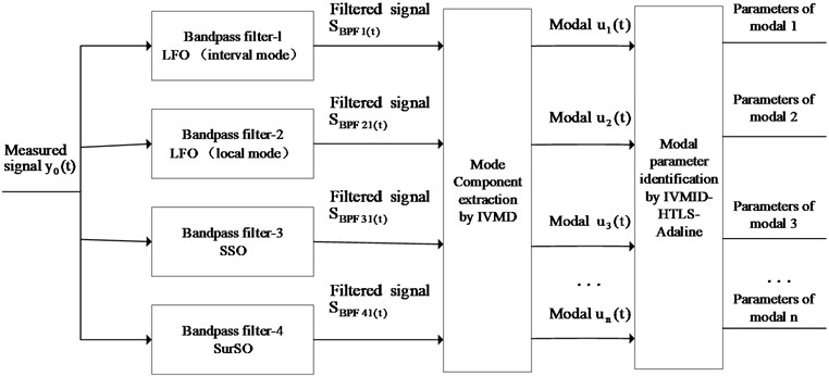
The framework for modal oscillations identification in a broad-band is shown in Fig. 1. The identification process is divided into the following three steps.

Step-1. Multiple Band Pass Filters (BPF) is used to decompose the original signal into multiple filtered signals in different frequency bands, so as to separate the oscillation signals.

Step-2. The IVMD algorithm is used to extract the oscillation modal signal from each BPF filtered signal.

Step-3. The HTLS-Adaline algorithm is used to identify the oscillation mode signals provided by IVMD, and obtain the information of each oscillation mode. The original signal is filtered through band-pass filtering, IVMD modal signal extraction and HTLS-Adaline identification to obtain modal parameters.

Fig. 1Framework of the mode identification for broad-band oscillation

3.1. Band-pass filter design

There are mainly three types of oscillations that cause power systems accidents: low-frequency oscillation, sub-synchronous oscillation and super-synchronous oscillation. The low-frequency oscillation is further divided into local mode and interval mode. The frequencies of each type of oscillations are in different ranges. Thus, this article designs four BPFs. A proper signal length selection can improve the accuracy of pattern recognition and ensure the rapidity of recognition. Because each oscillation frequency is different, it is obviously inappropriate to use the same length of data for identification. Table 1 shows the BPF filter bandwidth and identification sampling time corresponding to various oscillations in this paper.

According to the analysis of the modal identification algorithm [31], if it is necessary to obtain the oscillation frequency and amplitude more accurately, the sampling time of the identification signal must be greater than 1 oscillation period. In order to obtain accurate damping ratio information, the sampling time needs to be longer than two oscillation periods. Therefore, for low-frequency oscillations, in order to ensure rapid identification, the minimum band-pass frequency of the band-pass filter is 0.2 Hz, and the sampling time is selected to be twice the oscillation period, that is 10 s. For sub-synchronous oscillation, the identification speed is considered comprehensively. The minimum oscillation frequency is 10 Hz as the benchmark and the sampling time is 4 times. The oscillation period is 0.4 s. The mechanism of super-synchronous oscillation determines that it appears in pairs with sub-synchronous oscillation and the frequencies are complementary. The sampling time of the synchronous oscillation is the same as that of the sub-synchronous oscillation, and is also 0.4 s.

3.2. Modal signal extraction based on improved VMD algorithm

3.2.2. Determination of VMD penalty factor based on PSO algorithm optimization

The penalty factor $\alpha$ in the VMD algorithm has a great impact on the decomposition results. The study found that the smaller the penalty parameter $\alpha$, the larger the bandwidth of each IMF (Intrinsic Mode Function) component, and vice versa [32]. Therefore, when using VMD to decompose the oscillation signal of the power system, it is very important to choose the appropriate penalty factor parameter $\alpha$. In this paper, genetic mutation particle swarm optimization is used to optimize the penalty parameters to obtain the optimal $\alpha$.

Particle swarm optimization is a global optimization algorithm proposed by Eberh and Kennedy et al. in 1995. This method is a swarm intelligent optimization algorithm, and it has the advantages of few parameters, easy adjustment, and easy to fall into a local optimum. In order to obtain the global optimal approximate solution [33], this paper introduces the idea of genetic algorithm mutation in particle swarm algorithm to construct a genetic mutation particle swarm algorithm.

Definition of genetic mutation particle swarm algorithm: In an $D$-dimensional search space, label population $X$, and it is composed of m particles, $\mathbf{X}=[{\mathbf{x}}_1,{\mathbf{x}}_2,\cdots ,{\mathbf{x}}_m]$. The position of each particle in the search space can be represented by a $D$-dimensional vector, that is, ${\mathbf{x}}_i=[x_{i1},x_{i2},\cdots ,x_{iD}]$. $D$ is the number of parameters to be optimized, and the moving speed of $i$-th particle is ${\mathbf{v}}_i=[v_{i1},v_{i2},\cdots ,v_{iD}]$. The local extremum of particles is ${\mathbf{p}}_i=[p_{i1},p_{i2},\cdots ,p_{iD}]$; the global extremum of the population is ${\mathbf{G}}_1=[g_1,g_2,\cdots ,g_D]$, and the sub-global optimal value is ${\mathbf{G}}_2=[{g\text{'}}_1,{g\text{'}}_2,\cdots ,{g\text{'}}_D]$. The maximum individual optimal algebra is $\mathrm{m}\mathrm{a}\mathrm{x}Age$, and the mutation probability is$q$. In order to prevent particles from falling into the local optimum, it is necessary to record the individual optimal maintaining algebra of the particles during the iteration process. When the individual optimal maintaining algebra does not reach $\mathrm{m}\mathrm{a}\mathrm{x}Age$, each particle updates the position of the next generation by individual local extreme value and global extreme value. The formula is updated as:

6

${\mathbf{v}}_i^{n+1}=\omega {\mathbf{v}}_i^n+c_1\eta \left({\mathbf{p}}_i-{\mathbf{x}}_i^n\right)+c_2\eta \left({\mathbf{G}}_1-{\mathbf{x}}_i^n\right),$

7

${\mathbf{x}}_i^{n+1}={\mathbf{x}}_i^n+{\mathbf{v}}_i^{n+1}.$

In the formula, $\omega$ is the inertia weight; $\eta$ is a random number between [0, 1]; $c_1$ and $c_2$ are the learning factors respectively that represent the local search ability and the global search ability; $n$ is the number of iterations, and ${\mathbf{v}}_i$, ${\mathbf{p}}_i$, ${\mathbf{G}}_1$ and ${\mathbf{x}}_i$ are $D$-dimensional vectors respectively. The determination of the inertia weight $\omega$ of the current number of iterations adopts the linear decreasing weight method proposed by Shi [34], and the formula is as follows:

8

$\omega ={\omega }_{\mathrm{m}\mathrm{a}\mathrm{x}}-\frac{\left({\omega }_{\mathrm{m}\mathrm{a}\mathrm{x}}-{\omega }_{\mathrm{m}\mathrm{i}\mathrm{n}}\right)n}{n_{\mathrm{m}\mathrm{a}\mathrm{x}}}.$

In the formula, ${\omega }_{\mathrm{m}\mathrm{a}\mathrm{x}}$ and ${\omega }_{\mathrm{m}\mathrm{i}\mathrm{n}}$ are the maximum and minimum inertia weights; $n$ is the current number of iterations, and $n_{\mathrm{m}\mathrm{a}\mathrm{x}}$ is the defined maximum number of iterations. When the individual optimal retention algebra reaches $\mathrm{m}\mathrm{a}\mathrm{x}Age$, the genetic mutation operation is used to update the position and velocity of the particle to make it jump out of the local optimal. Selection of fitness function for genetic mutation particle swarm optimization algorithm: In the parameter optimization, the evaluation criterion of the decomposition effect of VMD method uses the concept of envelope entropy $E_p$ proposed by Tang Gui-ji et al. [35]. The envelope entropy of $x\left(j\right)$ time signal $c$ of length $N$ is defined as:

9

$E_p=-\sum _{j=1}^N{p}_j\log \left(p_j\right),p_j=a\left(j\right)/\sum _{j=1}^{N}a\left(j\right).$

In the formula, $a\left(j\right)$ is the envelope signal of $x\left(j\right)$ after Hilbert demodulation, and $j=\mathrm{1,2},\cdots ,N$. $p_j$ is the result of normalizing $a\left(j\right)$. Normalization not only avoids the influence of different envelope amplitudes of IMF components, but also reduces the interference of weak noise. $E_p$ is obtained according to the information entropy calculation rules. This article measures the decomposition effect of VMD according to $E_p$.

The VMD method is used to decompose the BPF filtered oscillation signal. When the component contains more noise, the sparseness of the component signal is weak and the envelope entropy is large. On the contrary, when a regular oscillation signal appears in the component, the signal will have strong sparseness, and the calculated envelope entropy is small at this time. Therefore, under the influence of parameter $\alpha$, the minimum entropy $E_p$ of the $K$ components is selected as the local minimum entropy $\mathrm{m}\mathrm{i}\mathrm{n}{E}_p$. The component corresponding to the minimum entropy value contains rich feature information. The local minimum entropy is used as part of the fitness function of the entire search process to find the parameter ${\alpha }_0$ corresponding to the global optimal component. Through the above analysis of parameter $\alpha$, a proper $\alpha$ will reduce the iterations of VMD, that is, the VMD method has a high decomposition efficiency. Therefore, it is necessary to achieve the highest decomposition efficiency in the case of the best decomposition effect. This article builds the fitness function based on $\mathrm{m}\mathrm{i}\mathrm{n}{E}_p$, add $time$ (iterations) as follows $\mathrm{m}\mathrm{i}\mathrm{n}F=\mathrm{m}\mathrm{i}\mathrm{n}{E}_p+\beta \cdot time$, where $\beta$ is the quantization factor of the fitness function.

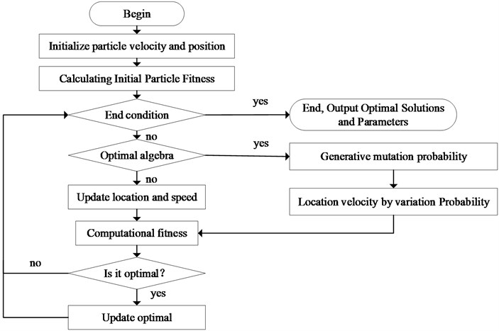
In this paper, the number of modal components $K$ and penalty factor $A$ in VMD decomposition are set as model hyper parameters. In the process of VMD optimization by PSO, the number of particle is set as 30, and the maximum number of iterations is set as 500.The learning factor is set as $c_1=c_2=$2; the velocity inertia factor is set as $w=$ 0.8, and the velocity coefficient is setas $\lambda =$ 1. The maximum and minimum inertia weights are set as ${\omega }_{\mathrm{m}\mathrm{a}\mathrm{x}}=$ 0.9 and ${\omega }_{\mathrm{m}\mathrm{i}\mathrm{n}}=$ 0.1 respectively, and the quantization factor of the fitness function is set as $\beta =$1/1000. The parameter optimization process based on genetic mutation particle swarm optimization algorithm is shown in Fig. 2.

Fig. 2Parameter optimization process based on genetic mulation particle swarm optimization

The BPF signal is decomposed by improved VMD to obtain the oscillation mode $u_n\left(t\right)$ extracted by VMD. When the accuracy of BPF and VMD is high enough, for modal signal $u_n\left(t\right)$, there is $u_n\left(t\right)\approx y_n\left(t\right)$.

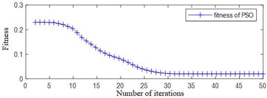
Therefore, through BPF and IVMD, all oscillation modal signals can be separated from the original signal. The convergence process of VMD optimization using PSO is shown in Fig. 3.

Fig. 3Convergence process of fitness function in VMD optimization by PSO

3.3. VMD-HTLS algorithm for frequency and attenuation factor

After the modal signals $u_n\left(t\right)$ are obtained by the IVMD decomposition, the HTLS algorithm is used to identify the modal parameters, such as the oscillation frequency and attenuation factor. HTLS algorithm is a subspace rotation invariant method, which has high computing efficiency and strong anti-noise ability. Its calculation steps are described in [29]. The main idea is to construct a Hankel matrix using the sampled signal, and perform Vander Mang decomposition on it. Using the translation-invariant characteristic of the van der Mun matrix to construct the equivalent relationship, and the eigenvalues of the oscillating modes are obtained. The main idea of IVMD-HTLS is: IVMD is used to decompose the BPF filtered sequence, and then the HTLS algorithm is used to calculate the oscillation frequency and attenuation factor for each component after decomposition. Because the FOMC-HTLS algorithm cannot give the amplitude and phase of the original signal $y\left(n\right)$, and the information of each mode is incomplete. It is not conducive to the reconstruction of the signal and the quantitative evaluation of the algorithm. Therefore, this paper introduces the Adaline God network to oscillate modal information (Amplitude and Phase).

3.4. Adaline neural network solves amplitude and phase

3.4.1. Adaptive linear neural network

Adaptive linear (Adaline) neural network is a neuron model proposed originally by Widrow and Hoff [36]. It is widely used in signal processing and other fields.

Fig. 4The principle of adaptive linear neural network

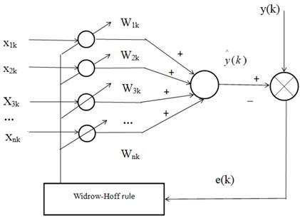
In Fig. 4, $x_{1k}$, $x_{2k}$,⋯, $x_{nk}$ are the $n$ input signals of the adaptive linear neural network at time$k$.The input signal vector form is expressed as ${\mathbf{X}}_{ik}=[x_{1k},x_{2k},\cdots ,x_{nk}{]}^T$, and this is often called the input pattern vector of Adaline neural network. The weight vector corresponding to each group of input signals is ${\mathbf{W}}_{ik}=[w_{1k},w_{2k},\cdots ,w_{nk}{]}^T$. The Adaline neural network output is:

10

$\widehat{y}\left(k\right)={\mathbf{X}}_{ik}^T{\mathbf{W}}_{ik}.$

Let $A$ be the ideal response signal, and define the error function as:

11

$e\left(k\right)=y\left(k\right)-\widehat{y}\left(k\right).$

The working process of Adaline neural network is as follows [36]: the ideal response signal $y\left(k\right)$ is compared with the output signal $\widehat{y}\left(k\right)$ of the neural network to obtain different $e\left(k\right)$. Feed$e\left(k\right)$into the learning rules, and adjust the weight vector according to the learning rules to make $\widehat{y}\left(k\right)$ and $y\left(k\right)$ consistent.

The learning rule of Adaline neural network is Widrow-Hoff rule, which is the least square error algorithm (LMS). The rule weight vector adjustment expression is:

${\mathbf{W}}_{i(k+1)}={\mathbf{W}}_{i(k+1)}+\eta e\left(k\right){\mathbf{X}}_{i\left(k+1\right)}.$

In the formula, $\eta$ is the learning rate of the Adaline neural network, $\eta \in \left(\mathrm{0,1}\right)$. Its value directly affects the weight vector adjustment accuracy and the convergence velocity.

4.1. Simulation analysis

In order to verify the effectiveness of the method in this paper, an oscillating signal $y_{test}$ is constructed by simulation:

In the formula: $y_{LFO1}$ is the low-frequency oscillation interval mode;$y_{LFO2}$ is the low-frequency oscillation local mode; $y_{SSO1}$ is the sub-synchronous oscillation and paired with the super-synchronous oscillation signal $y_{SurSO}$; $y_{SSO2}$ is another independent sub-synchronous oscillation, and $y_{Noise}$ is the white noise. In line with the real situation, the test signal satisfies the following conditions and assumptions: (1) All oscillation frequencies are randomly selected within the frequency band of the oscillation type; (2) Low frequency oscillation is the main mode of oscillation; the amplitude is higher than the sub-synchronous oscillation, and the local mode of low frequency oscillation is higher than the interval mode; (3) In the pair of sub-synchronous and super-synchronous oscillations, the amplitude of sub-synchronous oscillation mode is slightly higher than the super-synchronous mode. Based on the above assumptions, the specific parameters of each mode of the test signal are finally selected as:

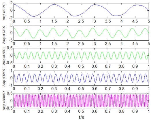
That is, the test signal $y_{test}$ contains 5 oscillating signals with different frequencies and a white noise signal with amplitude of 0.16. The frequency band of the test signal oscillation $y_{test}$ is 0.63-93.42 Hz. Each test signal is equal amplitude oscillation. The time domain form of the test signal $y_{test}$ is shown in Fig. 5. Using the proposed method after the constructed test signal $y_{test}$ is extracted by band-pass filtering and IVMD, the oscillation modal signals in each frequency band are shown in Fig. 6. It can be seen from Fig. 6 that the method proposed in this paper can accurately distinguish the modalities of different frequency bands and effectively extract all corresponding modal signals.

Fig. 5Test signal ytest

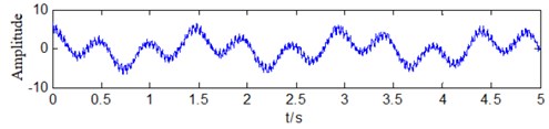
Fig. 6Mode signals extracted by IVMD

The modal signals are extracted for each IVMD obtained in Fig. 6, and the modal identification is performed through the HTLS-Adaline algorithm to obtain the parameter information of the corresponding modal. The identification results of this method compared with those of other methods is shown in Table 2. The selected comparison methods are: (1) the classic EMD-based HTLS algorithm (EMD-HTLS); (2) the VMD-based HTLS algorithm (VMD-HTLS); (3) the proposed method is based on the algorithm of IVMD-HTLS and Adaline (IVMD-HTLS-Adaline).

It can be seen from Table 2 that when the test signal oscillates in multiple frequency bands, the proposed method can effectively identify all oscillation modes. The maximum error of the oscillation frequency identification result is 1.55 %, with an average error of 0.67 %, and that of the oscillation amplitude identification result is 9.09 %, with an average error of 2.54 %. In comparison, the EMD-HTLS method has the worst frequency identification and amplitude identification results, and the average error is also the highest. The VMD-HTLS method has a good identification effect on the dominant oscillation mode ($y_{LFO2}$) with the highest amplitude. The frequency and amplitude identification results are close to those of this method, but the phase identification results are not as good as those of this method. For the sub-modes $y_{LFO1}$ and $y_{SSO1}$, the VMD-HTLS frequency identification effect is close to the proposed method, but the amplitude and phase identification results are far worse than it. In particular, for mode $y_{SSO2}$ with low amplitude and high frequency, the recognition results of EEMD-HTLS and VMD-HTLS are poor. For the super-synchronous oscillation mode $y_{SurSO}$ with a frequency of 93.42, the EEMD-HTLS method failed to identify it, and the result of VMD-HTLS is inconsistent with the actual one. Therefore, the method proposed in this paper has obvious advantages in identifying multi-mode coexisting pan-band oscillations.

4.2. Actual study data

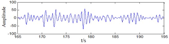
In order to prove the effectiveness of the proposed method, the actual oscillation data of Hunan Power Grid was selected and the oscillation mode identification analysis was carried out. The oscillation event is as follows: On June 24, 2018, a low-frequency oscillation occurred in a thermal power plant in Hunan Power Grid. The system started to oscillate at low frequency in the 120th second. After 30 s, the system quickly started to emit an alarm. The system maintained an alarm for about 180 s. In 60-120 s before the oscillation, the system has a noise-like oscillation, and the system did not issue an alarm at this time. The range of the oscillation signal and noise-like signal has been marked in the figure. The system sampling frequency is 100 Hz. The oscillation signal at 165-195 s is selected, and the modal identification of this method is adopted. The original signal used for identification is shown in Fig. 7.

It can be seen from Fig. 6 that the amplitude of the oscillation signal is high, and the highest frequency fluctuation exceeds 100 MW, which is higher than 30 % of the system output power. At this time, the signal is affected by a certain degree of noise. For the original oscillation signal data shown in Fig. 7, the modal signals are extracted by the proposed algorithm as shown in Fig. 8. This method decomposes three modes from the oscillation signal data, which are the main modes of the system oscillation. Among the three modes, the first mode has the highest amplitude and is the dominant oscillation mode. The extracted modal signals are linearly superimposed, and the reconstructed signals are shown in Fig. 8.

Fig. 7Original oscillation data used for mode identification

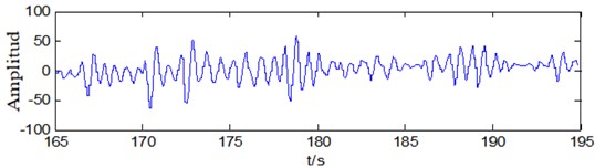
Fig. 8Mode signals extracted from the original oscillation data

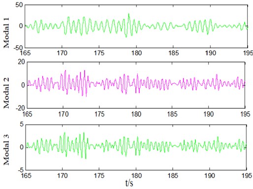
Fig. 9Reconstructed signal based on mode signals from IVMD

Comparing Fig. 9 with Fig. 7, it is not difficult to find that the reconstructed signal is basically the same as the original signal waveform. That is, the three modal signals separated cover the main oscillations of the system. The method in this paper can effectively extract all the main oscillation modal signals. Using the Prony algorithm to perform parameter identification on the modal signals in Fig. 6, the information of the main oscillation modes can be obtained. Table 3 compares the results of this method with the MF-Prony and EMD-Prony parameter identification results. It can be seen from the results that for the oscillation signal, both the proposed method MF-Prony or EMD-Prony can identify the mode with the largest amplitude. In the three methods, the MF-Prony frequency identification error is the highest, and the results of this method are similar to the EMD-Prony method. During the severe oscillation, the dominant modal frequency is about 1.48 Hz, and the minor dominant modal frequency is about 2.02 Hz.