Abstract
In wind turbines, rotating components serve as critical parts and are also prone to failures. The fault signals of wind turbines represent typical non-stationary and nonlinear signals susceptible to noise interference. Existing time-frequency analysis methods exhibit insufficient energy concentration when extracting time-varying non-stationary fault features, making feature extraction from signals more challenging. The primary drawbacks of single-data fault diagnosis methods lie in their limited information scope, poor robustness, lack of redundancy and fault tolerance, and difficulty in handling complex or multi-dimensional fault patterns. To address these issues, this paper proposed a model based on Improved TFMST and DSC-CNN-GRU. Firstly, the original Time-Frequency-Multisqueezing Transform (TFMST) technique was enhanced by optimizing its window function, introducing multi-scale adaptive thresholding to improve robustness, and relaxing the curvature criterion to enhance feature sensitivity. Furthermore, eps protection was incorporated throughout the algorithm to ensure numerical stability. Secondly, two datasets were constructed: one comprising two-dimensional data derived from the improved TFMST and the other containing one-dimensional raw data. Subsequently, a dual-input DSC-CNN-GRU model was developed, and both datasets were fed into it. Notably, the proposed model adopts a lightweight design. Finally, information from both data branches is fused and delivered to the classifier for the fault diagnosis task. To demonstrate the effectiveness of the proposed method, comparisons with other relevant methods were conducted on various datasets, indicating that the proposed method achieved desirable fault diagnosis accuracy.
Highlights
- A novel fault diagnosis model based on multimodal information fusion has been proposed.
- TFMST can generate a time-frequency representation of fault signals more concentrated energy.
- The model is capable of integrating time-frequency and temporal features.
- Experiments show that the proposed method is effective.
1. Introduction
Wind power is considered a green and sustainable energy option, playing a crucial role in the future transition of the energy structure [1, 2]. With the growing global focus on climate change, wind power will continue to play a vital role in contributing to the sustainable development of global energy [3, 4]. When wind drives the wind turbine blades to convert energy, due to the instability of wind speed, the strength and direction of the wind frequently change, resulting in intermittent and fluctuating characteristics. Components such as bearings, gears, and hubs, which are key power conversion elements of the turbine, often bear heavy loads and unloads. Additionally, due to prolonged exposure to complex natural environments during operation, these components are prone to various faults. These faults not only affect the normal operation of the wind turbine but can also lead to downtime, damage, energy waste, and even impact the surrounding environment and grid system [5, 6]. Therefore, fault diagnosis of wind turbines has become crucial, as it is an essential means to ensure the efficient, stable, and safe operation of wind farms. It helps improve the operational reliability of turbines, extend their service life, enhance power generation efficiency, reduce maintenance costs, ensure safe operation, and support the sustainable development of the entire wind energy industry [7].
Vibration signals are one of the most commonly used data sources in wind turbine fault diagnosis. The operation of wind turbines involves multiple complex systems and components, and any abnormality in a part can lead to performance degradation or failure. Through signal acquisition, real-time operational data can be collected, allowing for the analysis of parameter changes and timely identification of potential issues, thereby supporting fault diagnosis and prevention [8]. Traditional signal processing methods, such as Fourier Transform (FT) [9], Power Spectral Density (PSD) [10], and Autocorrelation Analysis [11], are effective for stationary signals. However, for non-stationary signals, these methods are unable to preserve their original characteristics. To address this issue, some time-frequency analysis (TFA) methods for non-stationary signals have gradually emerged, such as Short-Time Fourier Transform (STFT) [12], Wavelet Transform (WT) [13], Empirical Mode Decomposition (EMD) [14], and others. Although these methods can handle non-stationary signals, they also have a range of limitations. For example, the choice of window length in STFT is a key issue. A window that is too long will lose time-domain information, while a window that is too short will lose frequency-domain information. Additionally, the trade-off between frequency resolution and time resolution is a problem with STFT, as it cannot simultaneously describe both time and frequency characteristics of a signal accurately in time-frequency analysis. As the data scale continues to increase, it also leads to higher computational costs. Most time-frequency analysis methods typically face a trade-off between temporal resolution and frequency resolution. For complex dynamic signals from wind turbines, such as vibration signals and noise, this trade-off can result in fault features that are unclear or cannot be accurately extracted. Synchrosqueezing Transform (SST), proposed by Daubechies et al. in 2011 [15], is an effective time-frequency (TF) post-processing method. This approach significantly improves time-frequency resolution and can suppress low-level noise. However, it is primarily suitable for processing weak, time-varying signals. Building on this, Li et al. [16]. proposed the second-order adaptive synchrosqueezing transform (FSST) for non-stationary signals with rapid frequency variations, to enhance the time-frequency concentration and resolution of a multicomponent signal, and to separate its components more accurately. Wang et al. [17]. proposed a time-frequency analysis (TFA) method called the matching synchrosqueezing transform (MSST), which achieves a highly concentrated TF representation comparable to the standard TF reassignment methods (STFRM). Experimental results validated the effectiveness of MSST in mechanical fault diagnosis. Yi et al. [18]. addressed issues such as insufficient time-frequency energy concentration and frequent noise interference by combining multiple groups of wavelets with increased bandwidth into a super wavelet set and then proposed the Superlets Transform (SLT). By applying SLT to higher-order instantaneous frequency (IF) estimation and time-frequency energy rearrangement, they introduced the High-order Synchrosqueezing Superlets Transform (HSSLT) to achieve clearer and more concentrated time-frequency representations (TFR). This method was successfully applied to the bearing fault diagnosis of offshore wind turbines.
In recent years, fault diagnosis technologies for wind turbines based on deep learning methods have received widespread attention. For example, Deep Belief Networks (DBN) [19], Recurrent Neural Networks (RNN) [20], and Convolutional Neural Networks (CNN) [21] have been extensively used in fault diagnosis and have achieved promising diagnostic results. Li et al. [22]. proposed a method combining Deep Belief Networks (DBN) and 1D Convolutional Neural Networks (1D-CNN) for the one-dimensional raw fault signals of rotating machinery. This approach achieved dimensionality reduction, feature extraction, and classification of the fault data. Experimental results demonstrated the effectiveness of the method. Cao et al. [23]. proposed an intelligent fault diagnosis method based on Long Short-Term Memory (LSTM) networks for wind turbine gearbox faults. By comparing it with the Support Vector Machine (SVM) method, they verified the superiority of the proposed approach. Liu et al. [24]. proposed a novel method combining a one-dimensional (1-D) denoising convolutional autoencoder (DCAE) and a 1-D convolutional neural network (CNN) to address the issue of noise interference. Experimental results demonstrated that the method could achieve high-accuracy diagnosis even in noisy environments. Although fault diagnosis based on raw fault signals has shown some effectiveness, solely using one-dimensional signal analysis may overlook important time-frequency features, failing to capture the nonlinear and time-varying characteristics of the signal. To address these issues, methods that transform one-dimensional raw signals into two-dimensional time-frequency maps for wind turbine fault diagnosis have been continuously developed. These methods effectively overcome the limitations of traditional one-dimensional signal analysis, providing richer time-frequency feature information [25-27]. Zhang et al. [28]. transformed the one-dimensional raw signal into a two-dimensional time-frequency map using Short-Time Fourier Transform (STFT). By introducing the Scaled Exponential Linear Unit (SELU) function and combining it with a Convolutional Neural Network (CNN), they achieved classification of bearing faults. Jun et al. [29]. applied Variational Mode Decomposition (VMD) to decompose the raw signal and selected specific components. These selected components were then transformed into time-frequency maps using Continuous Wavelet Transform (CWT). By combining this approach with a Convolutional Neural Network (CNN), they successfully implemented fault diagnosis for rotating machinery. Shi et al. [30]. addressed the limitations of fault sample quantity and quality by transforming the one-dimensional raw signal into time-frequency maps using Short-Time Fourier Transform (STFT) and Synchronous Compressed Wavelet Transform (SWT). They combined these time-frequency maps with a Dual-Stream Convolutional Neural Network (DSCNN) and Support Vector Machine (SVM) to achieve mechanical fault diagnosis. This approach effectively leveraged the strengths of both CNN for feature extraction and SVM for classification, enhancing the diagnostic performance despite challenges with limited or noisy fault data. Che et al [31]. extracted time-domain features from vibration signals and transformed these features into multimodal samples consisting of grayscale images and time-series data. By combining CNN with models such as DBN, they implemented decision-level multimodal fusion to achieve comprehensive fault prediction results. The proposed method was validated through experiments, demonstrating its effectiveness in improving fault diagnosis performance by integrating different data representations and models. This approach highlights the advantage of combining time-domain features with deep learning models for more accurate and robust fault prediction. Yang et al. [32]. transformed the one-dimensional signals into two types of time-frequency maps using Gramian Angular Field (GAF) and Continuous Wavelet Transform (CWT) techniques to highlight fault features. They proposed a practical and effective Self-Attention Parallel Fusion Network (SAPFN) to achieve fault diagnosis for gearboxes. This approach effectively leveraged self-attention mechanisms to focus on key features in the data, improving diagnosis accuracy and robustness. Although transforming signals into time-frequency representations can enhance fault diagnosis accuracy, this approach demands substantial computational resources and time. Different fault modes may manifest as distinct frequency components, yet time-frequency representations often require compromises between frequency and temporal resolution, potentially leading to insufficient precision in capturing subtle fault signatures. The Time-frequency-multisqueezing Transform (TFMST) [33] method addresses these challenges while eliminating the energy diffusion issue at cross-components inherent to conventional methods, generating more focused time-frequency representations. This provides a novel approach to time-frequency data conversion. However, this method suffers from limitations including fixed threshold settings, inflexible window function parameters, and overly stringent curvature criteria.
Based on the above analysis and inspiration, this paper proposes a wind turbine unit fault diagnosis method based on the Improved TFMST and DSC-CNN-GRU model. The contributions of this paper are summarized as follows:
(1) Improvements were made to the original TFMST algorithm. Firstly, the window function parameter was optimized from 0.32 to 0.28 to better capture transient fault characteristics. Second, a breakthrough multi-scale adaptive threshold mechanism was introduced by integrating median threshold, maximum threshold, and baseline threshold, constructing an adaptive thresholding framework that addresses the sensitivity of fixed thresholds to outliers. Thirdly, the curvature criterion was relaxed to enhance feature detection sensitivity, effectively preserving subtle fault patterns. Finally, a 1:0.9 weighted energy allocation strategy was adopted to significantly suppress noise interference while maintaining feature integrity. A numerical stability protection mechanism was embedded throughout the algorithm to ensure robustness.
(2) This paper proposes a dual-input hybrid neural network DSC-CNN-GRU model that deeply integrates the advantages of CNN and GRU. The image input branch employs Deep Separable Convolution to replace traditional convolution, substantially reducing parameters while preserving feature extraction capabilities. The signal input branch effectively captures temporal features through a lightweight CNN and GRU. Feature summation enables the fusion of heterogeneous data information, allowing the model to simultaneously process spatial-visual information and temporal sequence signals.
The structure of this paper is as follows: Section 2 introduces the relevant theoretical foundations, primarily including the basic models of CNN and GRU. Section 3 presents the proposed fault diagnosis method. Section 4 describes the dataset used and the experimental setup. Section 5 validates and discusses the proposed method, demonstrating its effectiveness. Section 6 concludes the paper.
2. The proposed method
This section provides a detailed description of the proposed fault diagnosis method. First, the TFMST method is improved to obtain a more feature-rich time-frequency representation. Next, a Depthwise Separable Convolution-CNN-GRU Fusion Network model is proposed.
2.1. Improved TFMST
The fault signals of wind turbines are typically composed of various components such as harmonics, pulses, and frequency modulation. Commonly used TFA methods, such as STFT, WT, and Hilbert-Huang Transform (HHT) [34], are affected by the Heisenberg uncertainty principle, which requires a trade-off between time and frequency resolution. Attempting to accurately capture the instantaneous characteristics of the signal at a particular moment (i.e., increasing time resolution) may lead to a decrease in frequency resolution, and vice versa. The quantification of TF features requires the Instantaneous Frequency (IF) and Group Delay (GD) parameters. However, TF features are not completely independent time and frequency components, so a multi-compression approach is needed to effectively fuse the time and frequency information. TFMST method effectively integrates temporal and spectral information to generate a more concentrated TF feature representation. However, this method still exhibits certain limitations, as some fault features within the time-frequency representation may be lost. For instance, the original TFMST approach suffers from fixed threshold values, static window function parameters, and overly stringent curvature criteria. Building upon this foundation, the present study introduces enhancements to the TFMST algorithm addressing these aspects: thresholding strategy, window function parameters, curvature criteria, and numerical stability.
First, in the original algorithm, the Gaussian window parameter ( 0.32) resulted in deficient temporal resolution. For certain signals, this made it difficult to capture rapid transients within fault signals, adversely impacting feature extraction accuracy. To better capture transient faults and enhance sensitivity to weak fault signatures, the Gaussian window parameter was adjusted to 0.28. This modification controls the trade-off between temporal and frequency resolution:
where denotes the time coordinate.
In the original algorithm, the instantaneous frequency is estimated by directly employing division. Its instantaneous frequency estimate is given by:
where represents the frequency coordinate, denotes the STFT of the signal, signifies the STFT of the signal convolved with the derivative of the window function, and is the scaling factor. Numerical instability can occur when the value is very small. Consequently, building upon the original algorithm, we incorporated an epsilon (eps) safeguard to prevent division-by-zero errors and ensure numerical stability. The modified instantaneous frequency estimate incorporating epsilon is expressed as:
where denotes the machine epsilon, preventing division by zero.
Furthermore, the original algorithm utilized a fixed threshold, setting points in the time-frequency matrix with magnitudes below 0.2 times the maximum value to zero. For diverse signals, this approach fails to adapt to variations in statistical characteristics. Concurrently, a fixed threshold can excessively suppress weak fault features and exhibits sensitivity to outliers, where a single large magnitude value could disproportionately influence the entire threshold level. To enhance the robustness of threshold setting and achieve a better balance between feature preservation and noise suppression, we implemented an adaptive thresholding scheme combining the median and maximum values. The threshold function from the original algorithm is defined as:
where , .
The improved threshold function incorporates multiple scaling thresholds, including the median threshold, maximum threshold, and base threshold. By leveraging the signal’s global statistical characteristics, the threshold is determined dynamically to adapt to the energy distribution of diverse signals.
The median threshold is defined as:
where 0.25. The median exhibits inherent robustness to outliers, representing the signal’s typical magnitude. The coefficient 0.15 is configured to preserve components exceeding a specified proportion of this characteristic amplitude.
The maximum threshold:
where 0.25, this constraint prevents the threshold value from becoming excessively high, thereby avoiding the suppression of significant signal components while maintaining effective noise reduction.
The base threshold:
where 0.1, this configuration ensures the threshold does not drop excessively low, thereby preventing the retention of extraneous noise components.
Adaptive threshold synthesis:
Improved Thresholding scheme:
where denotes the indicator function.
Thus, when signal quality is sufficiently high, . Under conditions of anomalous noise, provides upper-bound protection.
The curvature criterion serves to distinguish between signal-dominant components and noise-dominant components. It operates based on derivatives of instantaneous frequency and group delay. The curvature ratio, which characterizes local geometric properties in the time-frequency distribution, is defined as:
where represents the time derivative of instantaneous frequency, and denotes the frequency derivative of group delay.
The original algorithm employs a strict curvature condition, with the feature mask characterized by:
The application of stringent curvature criteria may result in excessive misclassification of valuable fault features as noise, particularly diminishing sensitivity to faults exhibiting slight frequency modulation. To enhance fault feature detection sensitivity and preserve discriminative time-frequency patterns, we implement relaxed curvature conditions with epsilon-based numerical safeguarding. Adjusting the curvature ratio threshold from 1.0 to 1.2 and reducing the group delay derivative constraint from 0.2 to 0.15 enables retention of signal components with mild nonstationarity, thereby improving fault feature detection rates. The relaxed feature mask is defined as:
where .
Improved signal separation:
In the final energy allocation scheme, the original algorithm assigns equal weights to both the frequency directional synchrosqueezing result and the time directional synchrosqueezing result. By reducing the weight assigned to the time directional result to 0.9, we effectively diminish noise introduced through temporal reallocation, yielding enhanced output clarity. The modified weight configuration is implemented as follows:
where component satisfies the curvature condition and exhibits high signal-to-noise ratio. Component potentially contains elevated noise levels; therefore, its assigned weight is reduced.
2.2. A depthwise separable convolution-CNN-GRU fusion network
CNN have been widely applied in the field of fault diagnosis, particularly for processing complex signals, images, and time-series data. Owing to their powerful capability for automatic feature extraction, CNN have demonstrated superior performance in scenarios where traditional methods encounter difficulties. Within the CNN architecture, convolutional layers, pooling layers, and fully connected layers constitute the three primary layer types [35, 36]. The Gated Recurrent Unit (GRU), an advanced variant of the Recurrent Neural Network (RNN), was introduced by Kyunghyun Cho et al. [37]. in 2014. Leveraging gating mechanisms, the GRU selectively updates its hidden state to capture essential information while discarding irrelevant details [38]. Compared to the Long Short-Term Memory (LSTM) [39] network, the GRU possesses a simpler structure and exhibits lower computational complexity. Depthwise separable convolution (DSConv)] [40] is an improved convolutional method that decomposes a standard convolution into two separate operations: depthwise convolution (DWConv) and pointwise convolution (PWConv). The specific process is illustrated in Fig. 1.
Fig. 1Depthwise separable convolution process
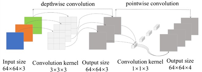
The distinction between DSConv and standard convolution lies in the fact that depthwise convolution employs single-channel kernels. It convolves each input channel separately, producing an output feature map with the same number of channels as the input. Subsequently, pointwise convolution (PWConv) with a kernel size of 1×1 is applied to increase dimensionality by aggregating information across all channels.
Assume the DWConv has a kernel size of , a number of kernels , and a parameter count of . Assume the PWConv has a kernel size of , a number of kernels , and a parameter count of . Therefore, the total parameter count for the DSConv is .
Whereas a standard convolution has a parameter count of , the parameter ratio between DSConv and standard convolution is . DSConv first performs DWConv independently on each input channel, then merges all channels into the output feature map via PWConv. This design achieves reduced computational cost and improved operational efficiency.
Based on relevant theoretical analysis and experimental validation, we propose a Dual-input Deep Separable Convolution-CNN-GRU Fusion Network (DSC-CNN-GRU) model. The proposed model primarily consists of two branches. Branch 1 is composed of standard convolutions and DSConv. The input data first undergoes preliminary feature extraction through a standard convolutional layer, followed by deeper feature extraction via two separable convolution modules. The function of Branch 1 is to extract features from image sample data. Branch 2 integrates a CNN model with a GRU model, where the CNN part adopts a lightweight design. This branch achieves feature extraction from one-dimensional data. Fig. 2 illustrates the specific structure of the proposed model.
Fig. 2The structure of depthwise separable convolution-CNN-GRU fusion network
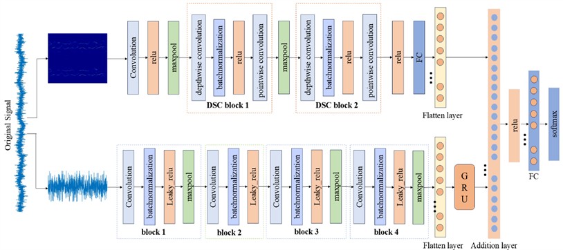
The proposed model’s Branch 1 primarily extracts features from the TFMST time-frequency diagrams. In this branch, the input first undergoes a convolution operation with a 5×5 kernel size, followed by feature extraction through two DSC blocks. Within these DSC blocks, the DWConv layers use kernel sizes of 3×3 and 5×5 respectively, and the PWConv layers use a kernel size of 1×1. Finally, the features are flattened via a fully connected layer and a flatten layer, with the purpose of fusing them with the features from Branch 2. Branch 2 primarily extracts features from the raw signal. This branch mainly consists of four convolutional blocks. The second convolutional block uses a kernel size of 1×1, while the other three blocks use a kernel size of 1×3. LeakyReLU is used as an activation function throughout Branch 2. Furthermore, max pooling is employed throughout the proposed model to reduce the dimensionality of the feature maps.
The network parameters and hyperparameter settings of the DSC-CNN-GRU model are shown in Table 1. In Branch 1, a 5×5 convolution kernel is first employed for initial feature extraction, with a stride of 2 to achieve downsampling. This rapidly reduces the spatial dimensionality and extracts fundamental visual features. The two DSC blocks decompose standard convolution into depthwise convolution and pointwise convolution. DSC Block 1 uses a 3×3 convolution kernel, significantly reducing computational load while maintaining feature extraction capability. DSC Block 2 employs a larger receptive field (5×5) to capture more complex feature patterns. In Branch 2, 1×3 convolution kernels are first used, specifically designed for processing temporal data. They perform local feature extraction along the temporal dimension while preserving channel integrity. This is followed by a 1×1 convolution for dimensionality reduction, then another 1×3 convolution for feature extraction, and finally a step to restore dimensions. This design significantly reduces the number of parameters and enhances nonlinear expressive power. Subsequently, 128 GRU units are utilized for temporal modeling to capture long-range dependencies within the sequential data. Only the output from the final timestep is taken, yielding a compressed representation of the entire sequence. Following feature extraction in both Branch 1 and Branch 2, the 128-dimensional feature vector from the Light-CNN branch (Branch 1) and the 128-dimensional feature vector from and the 128-dimensional feature vector from the GRU branch (Branch 2) undergo element-wise summation. This achieves deep integration of the visual and temporal features.
The total number of learnable parameters in the final proposed model is 2.5M. Compared to classical neural network models such as AlexNet [41] (approximately 60M parameters) and ResNet-18 [42] (approximately 11.7M parameters), the proposed model achieves a substantial reduction in parameters. This lightweight architecture significantly enhances training efficiency, paving the way for future applications in fault diagnosis.
Table 1Network parameters of DSC-CNN-GRU
Branch 1 | Activations | Learnables | Branch 2 | Activations | Learnables |
imageinput | 128×128×3 | – | datainput | 1×1024×1 | – |
conv_1 | 256×256×3 | Weights 5×5×3×6 Bias 1×1×6 | conv_4 | 1×1024×16 | Weights 1×3×1×6 Bias 1×1×16 |
relu_1 | 126×126×6 | – | bn_3 | 1×1024×16 | Offset 1×1×16 Scale 1×1×16 |
maxpool_1 | 126×126×6 | leaky_relu_4 | 1×1024×16 | – | |
conv_2_depthwise | 63×63×6 | Weights 3×3×6×6 Bias 1×1×6 | maxpool_3 | 1×511×16 | – |
bn_2 | 32×32×6 | offset1×1×6 scale1×1×6 | conv_5 | 1×511×16 | Weights 1×1×16×16 Bias 1×1×16 |
relu_2 | 32×32×6 | – | bn_5 | 1×511×16 | Offset 1×1×16 Scale 1×1×16 |
conv_2_pointwise | 32×32×6 | Weights 1×1×6×120 Bias 1×1×120 | leaky_relu_5 | 1×511×16 | – |
maxpool_2 | 32×32×120 | – | conv_6 | 1×511×32 | Weights 1×3×16×32 Bias 1×1×32 |
conv_3_depthwise | 16×16×120 | Weights 5×5×120×6 Bias 1×1×6 | bn_6 | 1×511×32 | – |
bn_3 | 8×8×6 | offset1×1×6 scale1×1×6 | leaky_relu_6 | 1×511×32 | Offset 1×1×32 Scale 1×1×32 |
relu_3 | 8×8×6 | - | maxpool_6 | 1×254×32 | |
conv_3_pointwise | 8×8×6 | Weights 1×1×6×120 Bias 1×1×120 | conv_7 | 1×254×32 | Weights 1×3×32×32 Bias 1×1×32 |
relu_4 | 8×8×120 | – | bn_7 | 1×254×32 | Offset 1×1×32 Scale 1×1×32 |
fc_1 | 8×8×120 | Weights 128×7680 Bias 128×1 | leaky_relu_7 | 1×254×32 | – |
flatten_1 | 1×1×128 | - | maxpool_7 | 1×126×32 | – |
flatten_2 | 4032 | – | |||
gru | 128 | Input weights 384×4032 Recurrent weights 384×128 Bias 384×1 | |||
Addition | 128 | ||||
relu_8 | 128 | ||||
fc_2 | 16 Weights 16×128 Bias 16×1 | ||||
Softmax | 16 | ||||
Classification | 16 | ||||
2.3. The proposed fault diagnosis method
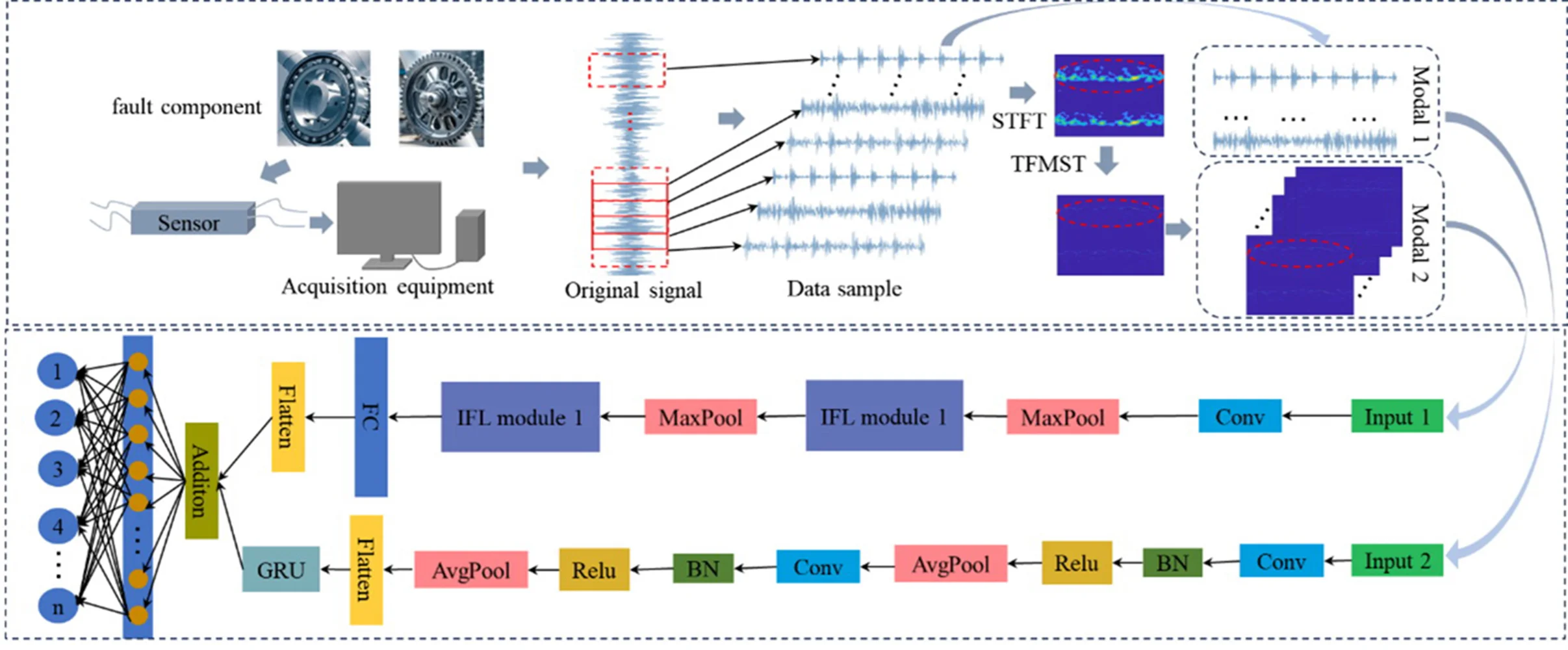
Building upon the methods and models described above, the enhanced TFMST time-frequency data and the raw fault data are utilized as two distinct fault datasets. These dual-modal inputs are simultaneously fed into the DSC-CNN-GRU hybrid neural network model to perform fault diagnosis. the diagnostic workflow is illustrated in Fig. 3.
Fig. 3Fault diagnosis procedure based on the DSC-CNN-GRU model
The specific procedural steps are as follows:
Step 1: Data Processing. Preprocess the raw fault data to facilitate subsequent analysis.
Step 2: Data Transformation. Address limitations in the original TFMST method including fixed thresholds, fixed window function parameters, and strict curvature criteria by employing the improved TFMST method. This generates 2D time-frequency diagrams with enhanced energy concentration and richer feature representation. Process the raw data through two distinct methods to obtain two different data types.
Step 3: Sample Division. Includes two data types corresponding to two sample sets. The first sample set contains improved TFMST 2D time-frequency diagrams. The second sample set contains raw fault data. Divide both sample sets into training and testing subsets according to a specified ratio.
Step 4: Model Construction and Hyperparameter Configuration. Construct the DSC-CNN-GRU model and configure its hyperparameters. This model comprises two pathways to achieve feature fusion across different data types.
Step 5: Model Training. Input the image dataset into Branch 1 for training. Simultaneously input the raw dataset into Branch 2 for training. Achieve fault classification through complementary feature extraction and feature fusion between both branches. Step 6: Model Testing. Evaluate the trained network using testing subsets. Obtain classification accuracy metrics for each fault type.
3. Experiment and data
In this section, the specific details of the experimental setup, the data and its processing, as well as the experimental setup and parameter settings are introduced. The evaluation metrics used to assess the algorithm model are also discussed.
3.1. Experiment
To validate the effectiveness of the method proposed in this study, we used the Case Western Reserve University (CWRU) bearing dataset [43]. Experiments were then conducted and verified on the Jiangsu Normal University-Wind Turbine-1 (JSNU-WT-1) test bench. The specific details of the two experiments are as follows:
The CRWU datasets test bench is shown in Fig. 4. The test bench mainly consists of four parts: the motor, torque sensor/encoder, power meter, and an electronic controller. The bearing to be tested is connected to the motor shaft, with the drive-end bearing model being SKF6205 and the fan-end bearing model being SKF6203. This study focuses on the drive-end SKF6205 bearing, with a system sampling frequency of 12 kHz. The fault points on the bearing are created through electrical discharge machining, with fault damage diameters of 0.1778 mm, 0.3556 mm, and 0.5334 mm. There are three fault locations on the bearing: Inner Race Fault (IR), Rolling Element Fault (RE), and Outer Race Fault (OR). Therefore, the bearing fault states are categorized into 9 fault states and 1 normal state, making a total of 10 bearing states. The vibration data was collected using an accelerometer, which was fixed to the housing with a magnetic base. The accelerometer was placed at the 12 o’clock position on both the motor housing drive-end and the fan end. All data were collected under different motor load conditions (0, 1, 2, and 3 hp). This study utilizes drive-end data acquired under 0hp load conditions with sampling frequencies of 12 kHz and 48 kHz as experimental data.
Fig. 4CRWU test bench [43]
![CRWU test bench [43]](https://static-01.extrica.com/articles/25113/25113-img4.jpg)
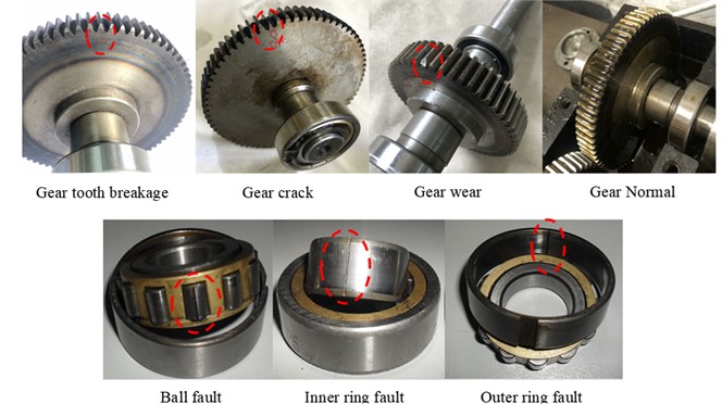
The design of the wind turbine fault simulation test bench is shown in Fig. 5 [1, 3]. The experimental data are obtained from the JSNU-WT-1 test bench, and the main research object of this experiment is the rolling bearings at the input end of the wind turbine gearbox. In order to simulate different types of bearing faults, these bearings are artificially damaged using wire electrical discharge machining (WEDM) technology to simulate various possible fault conditions. The entire testing process is precisely controlled by a control cabinet to ensure the stability of the experimental environment. During the experiment, the motor drives the planetary gearbox via a coupling, and the planetary gearbox is connected to the wind generator through a synchronous belt, thereby driving the generator to operate. The system’s rotational speed is regulated by a frequency converter, allowing for precise control of the speed. The signal acquisition system uses the INV3062T0 signal acquisition device, responsible for collecting various data from the entire system. for vibration signal acquisition, four INV9822 accelerometers are used, mounted on the gearbox housing and fixed with magnetic bases. The sampling frequency of the accelerometers is set to 4 kHz to ensure accurate capture of high-frequency signals. The core hardware configuration of the test bench includes a 400 W-rated generator, a 750 W-rated three-phase asynchronous motor, and an XW90 planetary gearbox with a gear ratio of 3. Through the combination of real wind turbine generators and transmission systems, the test bench simulates the actual operating environment of the wind turbine, aiming to closely replicate the true operating conditions of the wind turbine in order to obtain more accurate and meaningful experimental data. This experiment configures seven distinct bearing fault types, encompassing faults in two different components (bearings and gears), specifically comprising three gear fault variants, three bearing fault variants, and one healthy gear condition. The precise fault locations are illustrated in Fig. 6 [1, 3].
Fig. 5JSNU-WT-1 test bench
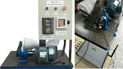
Fig. 6Wind turbine bearing failure in different locations
3.2. Data processing
We perform sliding window sampling on the data collected as described above, which helps to improve the accuracy of both time-domain and frequency-domain analysis, reduce the boundary effects caused by signal segmentation, and enhance the ability to capture the details of the signal. Each signal segment comprises 1024 data points. for the CWRU dataset, the sliding window step size is 512, with an overlap of 512 between adjacent segments, as illustrated in Fig. 7. for the JSNU-WT-1 dataset, a reduced step size of 200 is adopted to increase sample quantity, resulting in an overlap of 824 between signals. CWRU dataset encompasses 16 distinct bearing health states. Each state contains 200 samples, yielding a total of 3,200 samples. These 16 bearing fault types have been systematically labeled; detailed specifications are provided in Table 2. JSNU-WT-1 dataset includes 7 bearing fault conditions. Each condition comprises 200 samples, resulting in 1,400 total samples. These 7 bearing and gear fault types have undergone labeling procedures; comprehensive information is documented in Table 3.
Fig. 7Example of raw data split into n samples
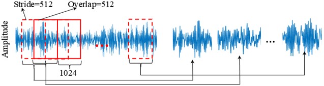
Table 2Composition of the CWRU bearing dataset
Fault type | Fault diameter (Inch)/ Sampling frequency (kHz) | Number of samples | Label |
BF007 | 0.007/12 kHz | 200 | 0 |
BF014 | 0.014/12 kHz | 200 | 1 |
BF021 | 0.021/12 kHz | 200 | 2 |
IR007 | 0.007/12 kHz | 200 | 3 |
IR014 | 0.014/12 kHz | 200 | 4 |
IR021 | 0.021/12 kHz | 200 | 5 |
OR007 | 0.007/12 kHz | 200 | 6 |
OR014 | 0.014/12 kHz | 200 | 7 |
OR021 | 0.021/12 kHz | 200 | 8 |
BF007 | 0.007/48 kHz | 200 | 9 |
BF021 | 0.021/48 kHz | 200 | 10 |
IR007 | 0.007/48 kHz | 200 | 11 |
IR021 | 0.021/48 kHz | 200 | 12 |
OR007 | 0.007/48 kHz | 200 | 13 |
OR021 | 0.021/48 kHz | 200 | 14 |
Normal | 0 | 200 | 15 |
Table 3Composition of the JSNU-WT-1 fault dataset
Fault type | Number of samples | Label |
Gear tooth breakage | 200 | 0 |
Gear crack | 200 | 1 |
Gear wear | 200 | 2 |
Ball fault | 200 | 3 |
Inner ring fault | 200 | 4 |
Outer ring fault | 200 | 5 |
Gear Normal | 200 | 6 |
3.3. Experimental setup and parameter settings
To enhance the model’s capacity for integrating heterogeneous data, strengthen the network’s representational capability and diagnostic accuracy, while improving system robustness and reliability, this study converts raw 1D signals into 2D time-frequency representations using an improved TSMST method. These transformed images exhibit richer features and concentrated energy distribution, forming the input for Branch 1 with dimensions of 256×256. The original 1D data serves as input for Branch 2 with dimensions of 1×1024. The dual-path architecture fuses these distinct data modalities to deliver comprehensive and precise fault diagnosis capabilities. The algorithmic parameters are configured as follows: initial learning rate = 0.0005, optimizer = Adam, batch size = 256, MaxEpochs = 20, L2 regularization parameter = 0.01, with softmax as the classifier.
In this paper, the parameters of all models are uniform. The algorithm was implemented using MATLAB. The computer used has an i5-12500H CPU and Windows 11 operating system. Additionally, the dataset was split, with 80 % used as the training set and 20 % used as the test set.
3.4. Performance evaluation metrics
In this study, to evaluate the advantages of the proposed algorithm model, we use four metrics: accuracy, recall, precision, and F1-score. Accuracy is the proportion of correctly predicted samples to the total number of samples in a classification model. It reflects the overall performance of the model across all samples and is suitable for cases with balanced data distribution. Recall measures the proportion of actual positive samples that the model correctly predicts as positive. in other words, it indicates how many of the actual positive samples the model is able to identify. Precision measures the proportion of predicted positive samples that are actually positive. in other words, it indicates how many of the samples predicted as positive by the model are truly positive. F1-score is the harmonic mean of precision and recall, considering the balance between the two. The F1-score is especially useful in cases of class imbalance, as it provides a trade-off between precision and recall. By combining both precision and recall, the F1-score offers a more comprehensive evaluation of model performance, and it provides a more reliable assessment, especially when the distribution of positive and negative classes is uneven. The definitions of these four metrics are as follows:
where (True Positive) represents that a positive sample is correctly predicted to be positive, (True Negative) represents that a negative sample is correctly predicted to be negative, (False Positive) represents a Negative sample being incorrectly predicted as a positive, and (False Negative) represents a positive sample being incorrectly predicted as a negative.
4. Results and discussion
In this section, we conducted two case studies to verify the performance and robustness of the proposed method in fault diagnosis tasks. Additionally, to eliminate experimental randomness, we performed 5 independent experiments for each method and took the average as the final result.
4.1. Case 1: CRWU dataset fault diagnosis
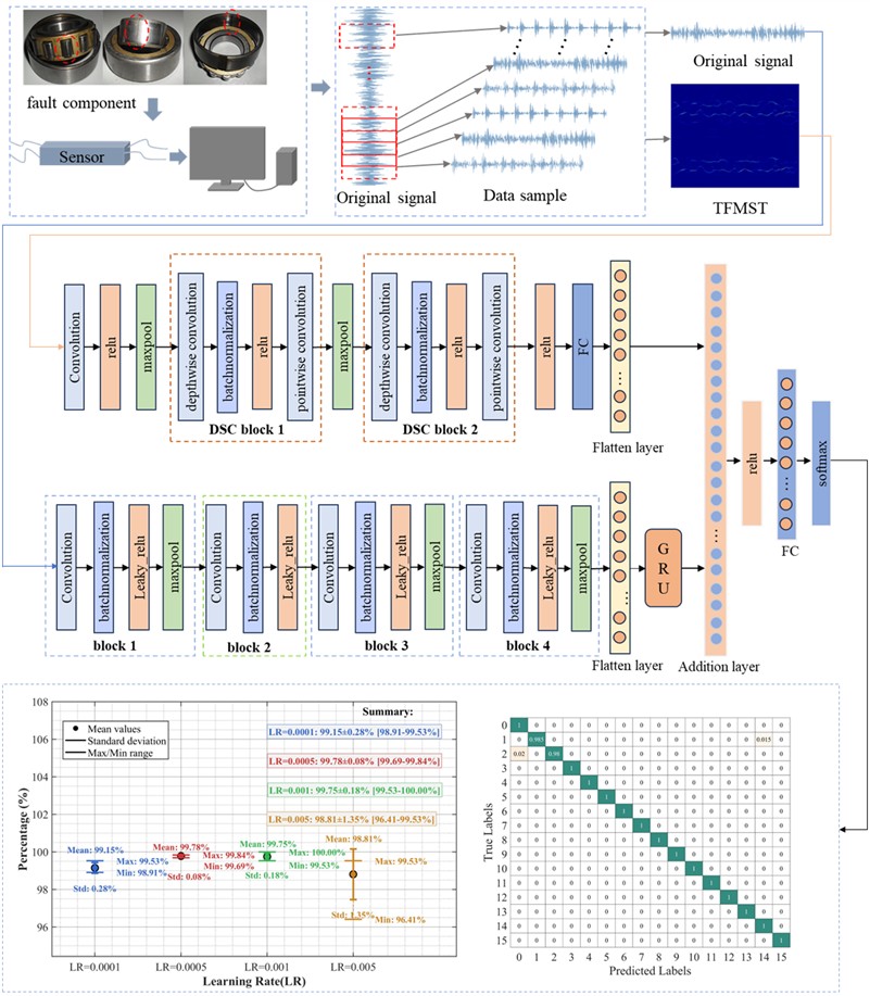
4.1.1. The impact of different learning rates on model performance
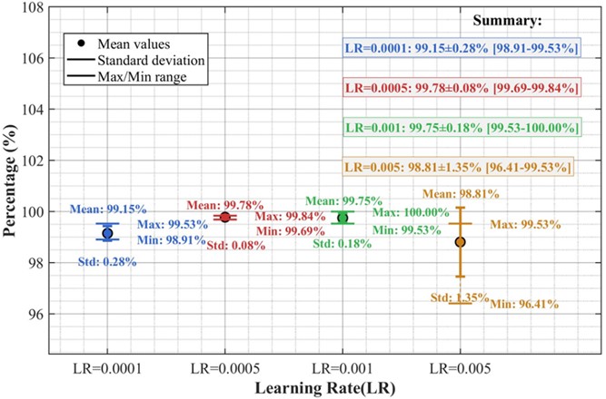
Generally, Learning Rate (LR) significantly influence model performance as they directly control the step size for parameter updates during training. Excessively large LR prevent loss function convergence and may cause oscillation near optimal values. Conversely, excessively small rates lead to slow convergence, requiring more training epochs. Thus, selecting an appropriate LR is critical. This study tested four learning rates (0.0001, 0.0005, 0.001, and 0.005) for model training and evaluation. Fig. 8 illustrates classification performance metrics across these learning rates, including mean accuracy, standard deviation (std), and maximum/minimum values from all trials. Results indicate that the proposed model achieved peak average accuracy (99.78 %) with LR = 0.0005, accompanied by the lowest std (0.08 %), demonstrating optimal stability. Although LR = 0.001 yielded perfect classification (100 %) in one trial, its mean accuracy (99.75 %) and std (0.18 %) were inferior to the LR = 0.0005 configuration.
Fig. 8Performance comparison of the model under different learning rates
4.1.2. Comparison with different data types
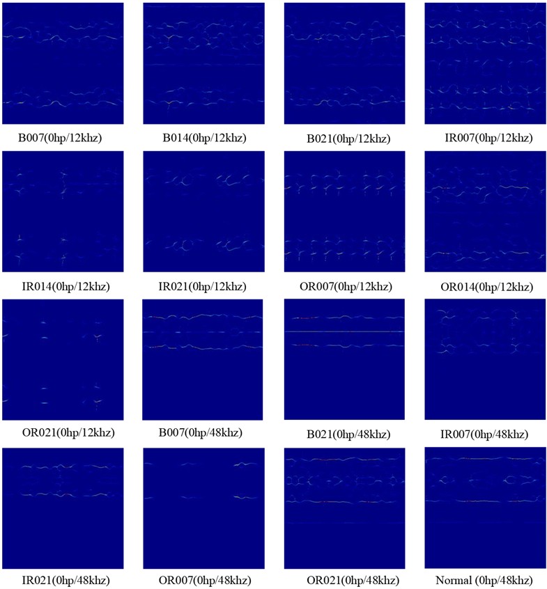
To highlight the advantages of the improved method, we transformed the one-dimensional raw signal into time-frequency diagrams using both the improved TFMST and the original TFMST methods, resulting in two fault samples. These samples, along with the raw signal, were used for training and testing the proposed model. Fig. 9 shows the time-frequency diagram of different fault categories obtained using the improved TFMST method. Fig. 10 shows the time-frequency diagram obtained using the original TFMST method. Fig. 9 and 10 represent different representations of the same signal. From the figures, it can be observed that the time-frequency diagram obtained using the improved TFMST method contains more features, which will benefit the diagnostic accuracy of the model.
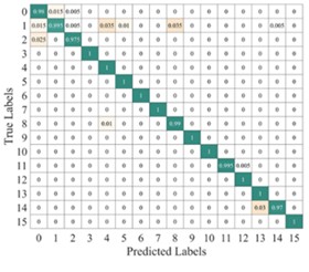
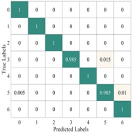
Fig. 11 shows the average confusion matrix of the time-frequency diagrams obtained using two different methods tested on the proposed model. From the figure, it can be observed that the improved TFMST data only has the possibility of misclassification between fault categories 2 and 3 in the model. in contrast, the original TFMST data shows the possibility of misclassification for four fault categories, including category 1, category 2, category 3, and category 15. Additionally, there is confusion between fault categories 2 and 3. This indicates that the time-frequency diagram obtained using the improved TFMST method contains more features, resulting in better diagnostic accuracy in the model.
Fig. 9Improved TFMST Time-Frequency diagrams for different fault types
4.1.3. Comparison with different models
The DSC-CNN-GRU model incorporates two distinct branches: Branch 1 constitutes a lightweight pathway employing DSConv, while Branch 2 integrates CNN and GRU architectures with a similarly lightweight design approach. Consequently, the proposed model can be modularized into two sub-models denoted as Light-CNN and CNN-GRU. The LeNet-5 and AlexNet models represent classical CNN architectural paradigms characterized by differing computational complexities and historical significance, serving as benchmark references for foundational deep learning frameworks.
Fig. 10Original TFMST time-frequency diagrams for different fault types
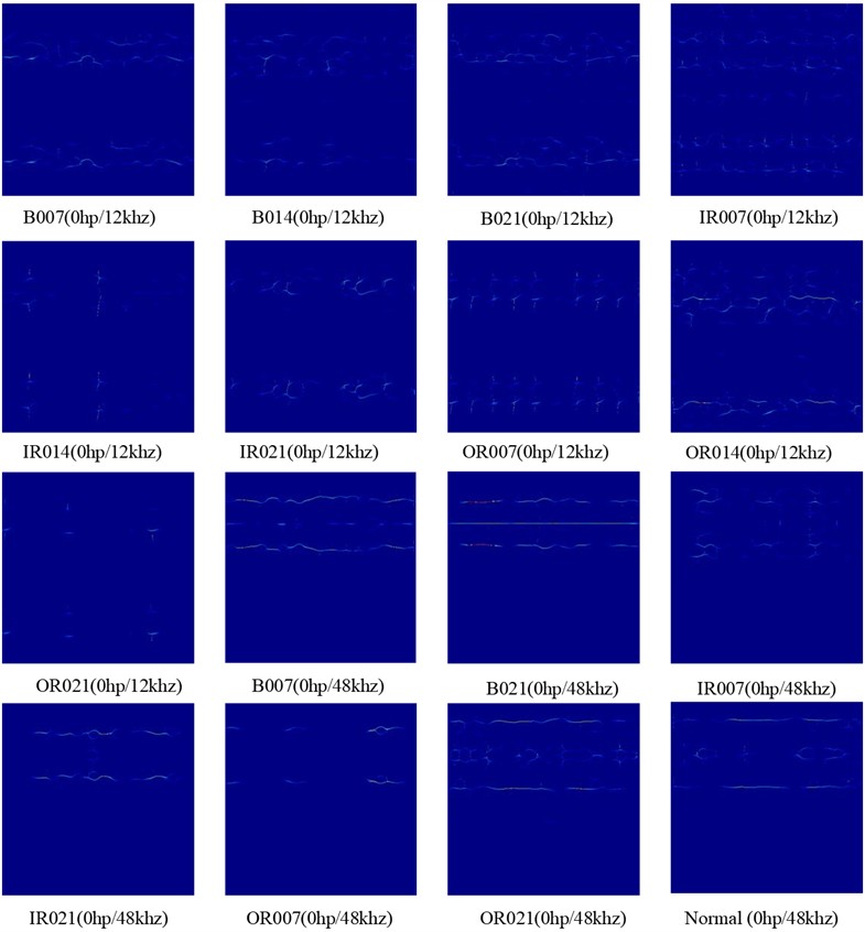
Fig. 11Average confusion matrix of test results from different methods on the proposed model
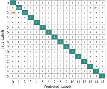
a) Average confusion matrix results of the improved TFMST method
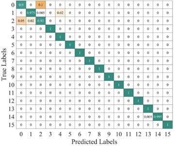
b) Average confusion matrix results of the original TFMST method
To demonstrate the superiority of the proposed model, these four architectures were established as comparative baselines, creating a comprehensive evaluation spectrum spanning elementary to advanced implementations and lightweight to relatively heavyweight configurations. This systematic comparison highlights the proposed model’s exceptional advantages in balancing performance and computational efficiency.
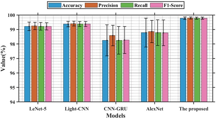
To highlight the advantages of the proposed model, we analyzed the results of multiple tests on the model using different metrics, including accuracy, precision, recall, and F1-score, as shown in Table 4. To provide a clearer comparison of the models' performance, we visualized these results in Fig. 12. The CNN-GRU and AlexNet models exhibited large standard deviation (std) fluctuations, indicating poorer model stability. Additionally, the average diagnostic accuracy of these two models was lower than that of the other models. in comparison to the LeNet-5 model, the Light-CNN model demonstrated higher stability and diagnostic accuracy. Notably, the proposed model achieved the highest diagnostic accuracy and best overall performance, with an accuracy of 99.78 %.
Table 4Performance comparison of different models
Model | Accuracy (%) | Precision (%) | Recall (%) | F1-score (%) |
LeNet-5 | 99.22±0.2923 | 99.25±0.2533 | 99.22±0.2615 | 99.22±0.2533 |
Light-CNN | 99.38±0.1914 | 99.40±0.1693 | 99.40±0.1693 | 99.38±0.1720 |
CNN-GRU | 98.25±1.0678 | 98.58±0.7086 | 98.25±0.9550 | 98.27±0.9351 |
AlexNet | 98.78±0.9968 | 98.86±0.7646 | 98.78±0.8916 | 98.77±0.8915 |
The proposed | 99.78±0.0856 | 99.79±0.0747 | 99.78±0.0765 | 99.78±0.0865 |
Fig. 12Visualization comparison of the performance of different models
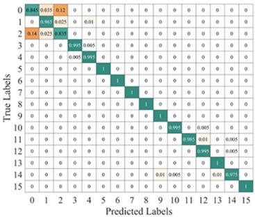
To further illustrate the diagnostic performance of different models on various fault categories, we plotted the average confusion matrix of the test results for each model, as shown in Fig. 13. The LeNet-5 model shows a potential for misprediction in five fault categories: categories 1-3, category 8, and category 15. The Light-CNN model has the possibility of misprediction in categories 1-4, but its accuracy is higher than that of the LeNet-5 model. The CNN-GRU model carries a risk of misprediction for categories 2-3, category 5, and category 15. The AlexNet model has the potential for misprediction across all six fault categories, resulting in the lowest prediction accuracy. in contrast, the proposed model only has a slight misclassification risk for faults in categories 2 and 3. Therefore, the proposed model demonstrates better performance, which is consistent with the results shown in Fig. 12.
Fig. 13Average confusion matrix of test results from different models
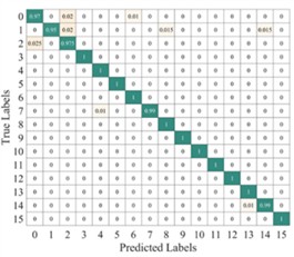
a) Lenet-5
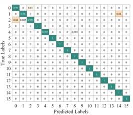
b) Light-CNN
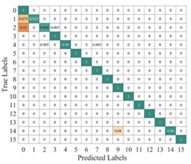
c) CNN-GRU
d) AlexNet
e) The proposed method
4.1.4. The effect of additional noise on model performance
Due to the complex operating environment of wind turbines, which is influenced by various environmental factors, the collected data can be affected by noise. in some harsh conditions, the impact of noise on the signal can be extremely severe. We added Gaussian noise with different signal-to-noise ratios (SNR) to the collected raw data to verify the classification performance of the proposed model under significant noise interference. the SNR can be defined as:
where and are the original signal power and noise power, respectively. A smaller SNR value indicates stronger added noise and greater interference with the original signal. This presents a challenge for fault diagnosis models.
The proposed model, as a dual-input model, increases the input dimension of the network, allowing the model to learn potential patterns and relationships in the data from different perspectives. This structure enhances the model's expressive power, especially when dealing with complex input data, providing stronger generalization ability compared to single-input models. We added noise with different SNRs to the raw data and generated two image datasets using TFMST and the improved TFMST methods. Then, we performed comparative experiments on the proposed model using both datasets. The results are shown in Table 5, and we visualized these results. Fig. 14 displays the comparison of the two methods on accuracy, precision, recall, and F1-score under different SNR conditions. It can be observed that, under all conditions, the proposed model consistently demonstrated higher performance. Fig. 15 presents the average confusion matrix of the proposed model’s test results under the conditions of SNR = 0 dB and 15 dB with the original data. From the figure, it is evident that, although the proposed method predicts more fault categories incorrectly than the original method under different conditions, its overall prediction accuracy remains higher than that of the original method. Therefore, the proposed model demonstrates superior diagnostic performance with the improved TFMST data.
Fig. 14Visualization of comparative performance of different data on the proposed model under varying SNRs
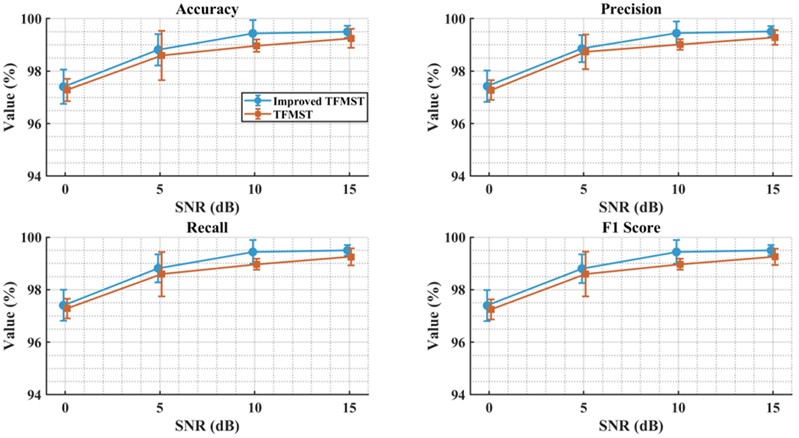
Fig. 15Average confusion matrix of the proposed model’s test results under different SNR conditions
a) TFMST SNR = 0 db
b) Improved TFMST SNR = 0 db
c) TFMST SNR = 15 db
d) Improved TFMST SNR = 15 db
Table 5Comparison of different signal-to-noise ratio data on the proposed model
SNR (dB) | Method | Accuracy (%) | Recall (%) | Precision (%) | F1-score (%) |
0 | Improved TFMST | 97.41±0.6592 | 97.43±0.5938 | 97.41±0.5896 | 97.40±0.5938 |
TFMST | 97.28±0.4222 | 97.28±0.3748 | 97.28±0.3776 | 97.24±0.3818 | |
5 | Improved TFMST | 98.81±0.6011 | 98.86±0.5128 | 98.81±0.5376 | 98.80±0.5467 |
TFMST | 98.60±0.9440 | 98.73±0.6579 | 98.60±0.8443 | 98.60±0.8491 | |
10 | Improved TFMST | 99.44±0.5015 | 99.44±0.4430 | 99.44±0.4485 | 99.44±0.4486 |
TFMST | 98.97±0.2370 | 99.01±0.2020 | 98.97±0.2119 | 98.97±0.2126 | |
15 | Improved TFMST | 99.50±0.2318 | 99.51±0.1979 | 99.50±0.2073 | 99.50±0.2078 |
TFMST | 99.25±0.3563 | 99.28±0.2849 | 99.25±0.3187 | 99.25±0.3168 |
4.1.5. Comparison with other relevant methods
To further demonstrate the superiority of the proposed method, we compared it with several related research methods that used the CWRU dataset. The comparison results of various methods are shown in Table 6. The number of fault categories used in this study is significantly higher than that in other methods. in general, the more fault categories there are, the more difficult the diagnosis becomes. Despite this, the proposed method still achieved the highest diagnostic accuracy. Specifically, the method [44] in classified the one-dimensional raw signal with an accuracy of 93.2 %, while the branch 2 (CNN-GRU) of the proposed model also classified the raw signal with an accuracy of 98.25 %. Therefore, the proposed method has certain advantages.
Table 6Comparison with related research methods
Methods | Fault types | Train dataset | Test dataset | Epoch | Accuracy |
1D convolutional neural network (1D-CNN) [44] | 6 | 409 | 605 | 100 | 93.2 |
Markov transition field and residual network (MTF+ResNet) [45] | 10 | 660 | 25 | 100 | 98.52 % |
Based on symmetrized dot pattern (SDP) images and convolutional neural networks (SDP + CNN) [46] | 10 | 240 | 60 | 150 | 98.88 % |
Two-stream feature fusion convolutional neural network (TSFFResNet-Net) (CWT+TSFFResNet-Net) [47] | 10 | 400 | 80 | 100 | 99.62 % |
The Proposed | 16 | 200 | 40 | 200 | 99.78 % |
4.2. Case 2: JSNU-WT-1 fault diagnosis
4.2.1. Comparison with different data types
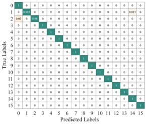
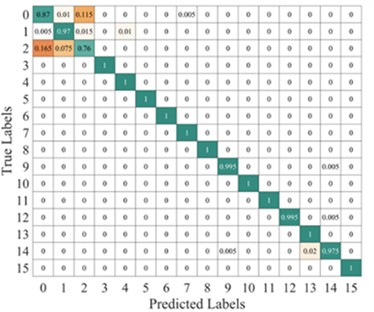
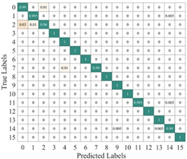
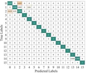
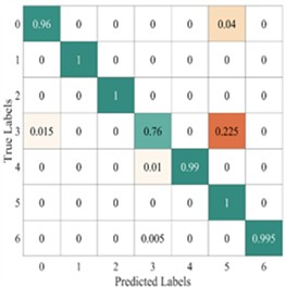
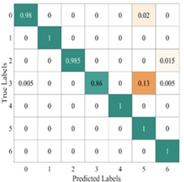
Fig. 16 and Fig. 17 show the time-frequency diagrams of the same signal for seven different fault types, obtained using the TFMST and the improved TFMST methods, respectively. From the figures, it can be observed that the time-frequency diagram obtained using the improved TFMST method contains more fault information. in general, the diagrams with rich information contribute to the correct predictions of the model. We input the two different datasets into the proposed model, and the average confusion matrix of the test results from both models is shown in Fig. 18. It can be seen that the proposed model demonstrated good diagnostic performance on the improved TFMST data. for the improved TFMST data, the proposed model only showed the possibility of misclassification for the ball fault and outer ring fault categories. for the original TFMST data, the model showed the possibility of misclassification for all fault categories. The proposed model exhibited excellent performance on the improved TFMST data.
Fig. 16Improved TFMST Time-Frequency diagrams for different fault types
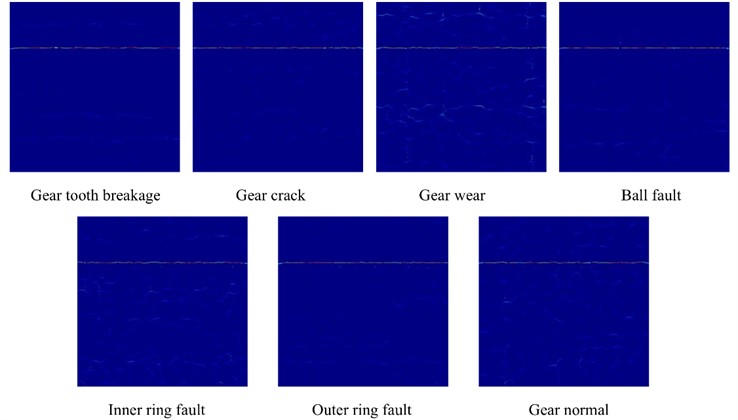
Fig. 17Original TFMST time-frequency diagrams for different fault types
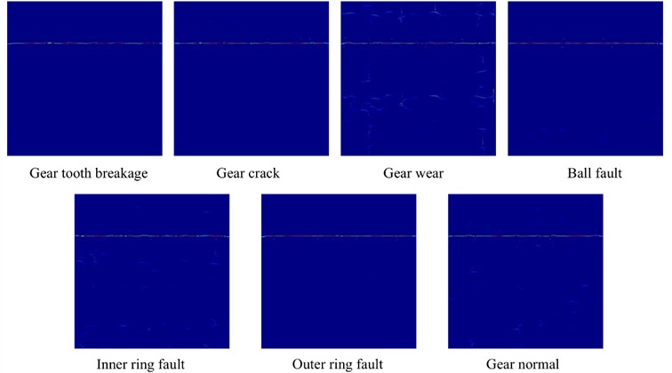
Fig. 18Average confusion matrix of test results from different methods on the proposed model
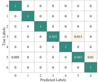
a) Average confusion matrix results of the improved TFMST method
b) Average confusion matrix results of the original TFMST method
4.2.2. Comparison with different models
To highlight the advantages of the proposed model, we compared it with LeNet-5, Light-CNN, CNN-GRU, and AlexNet. for the five different models, we compared the four metrics of accuracy, precision, recall, and F1-score, as shown in Table 7, and visualized the performance comparison of each model in Fig. 19. It can be seen that the metrics of the LeNet-5, Light-CNN, CNN-GRU, and AlexNet models are all lower than those of the proposed model, with LeNet-5, Light-CNN, and AlexNet models showing poor stability. Although the Light-CNN model exhibits good stability, its diagnostic accuracy remains lower than that of the proposed model.
Fig. 19Visualization comparison of the performance of different models
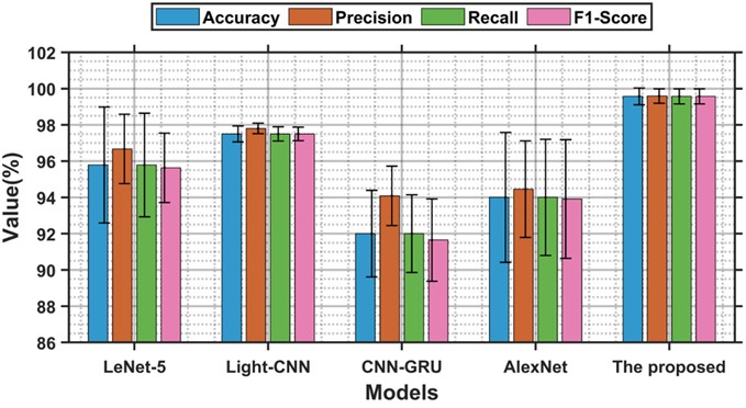
Fig. 20Average confusion matrix of test results from different models
a) Lenet-5
b) Light-CNN
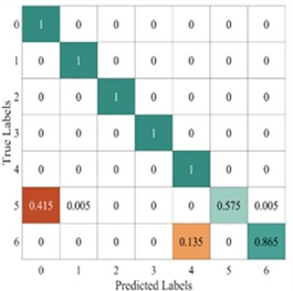
c) CNN-GRU
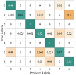
d) AlexNet
e) The proposed method
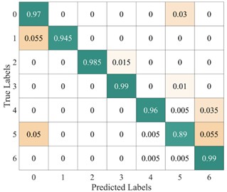
Fig. 20 shows the average confusion matrix of the test results from different models. The LeNet model correctly classified only the faults of the 2nd, 3rd, and 6th categories, while it had a risk of incorrect predictions for the remaining four fault categories, with the highest likelihood of error occurring for the 4th category. Similarly, AlexNet model only correctly predicted the faults of the 3rd and 5th categories, while errors occurred in the predictions of the remaining faults, making its performance the worst. Although Light-CNN and CNN-GRU demonstrated relatively high diagnostic performance, the proposed model outperformed them, delivering the best overall results and performance.
Table 7Performance comparison of different models
Model | Accuracy (%) | Precision (%) | Recall (%) | F1-score (%) |
LeNet-5 | 95.79±3.1984 | 96.67±1.9144 | 95.79±2.8607 | 95.63±1.9144 |
Light-CNN | 97.50±0.4374 | 97.80±0.2896 | 97.50±0.3912 | 97.50±0.3756 |
CNN-GRU | 92±2.3905 | 94.09±1.6417 | 92±2.1381 | 91.65±2.2714 |
AlexNet | 94.00±3.5839 | 94.46±2.6605 | 94.00±3.2055 | 93.91±3.2746 |
The proposed | 99.57±0.4657 | 99.59±0.3990 | 99.57±0.4165 | 99.57±0.4196 |
4.2.3. The effect of additional noise on model performance
To further validate the superiority of the proposed method, we added noise with different SNR values to the raw signal and obtained two different datasets using the improved TFMST method and the original TFMST method. We then conducted comparative experiments with these two datasets on the proposed model. The results were statistically analyzed using the four metrics: accuracy, precision, recall, and F1-score, as shown in Table 8. Additionally, to provide a clearer comparison, we visualized the experimental results, as shown in Fig. 21. From the results, it can be observed that under all conditions, the improved TFMST data exhibited higher performance on the proposed model and demonstrated greater stability.
Fig. 21Visualization of comparative performance of different data on the proposed model under varying SNRs
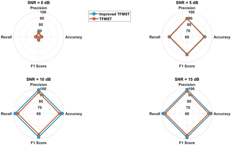
Table 8Comparison of different signal-to-noise ratio data on the proposed model
SNR (dB) | Method | Accuracy (%) | Recall (%) | Precision (%) | F1-score (%) |
0 | Improved TFMST | 64.714.5904 | 67.944.0644 | 64.714.0157 | 65.004.0644 |
TFMST | 64.433.7593 | 65.962.9316 | 64.43 | 64.533.1596 | |
5 | Improved TFMST | 88.074.8682 | 88.893.8397 | 88.074.3542 | 88.074.3809 |
TFMST | 87.293.4032 | 88.922.5271 | 87.293.0439 | 87.432.9494 | |
10 | Improved TFMST | 97.291.3505 | 97.351.1723 | 97.291.2080 | 97.281.2066 |
TFMST | 92.861.4940 | 93.551.0898 | 92.861.3363 | 92.881.3114 | |
15 | Improved TFMST | 97.930.6870 | 97.990.6188 | 97.930.6145 | 97.920.6269 |
TFMST | 94.502.3090 | 95.091.6802 | 94.502.0653 | 94.412.2183 |
5. Conclusions
To address the issues of incomplete feature extraction and low efficiency in wind turbine fault diagnosis, this paper proposes a fault diagnosis method based on the improved TFMST and DSC-CNN-GRU model. First, the improved TFMST technique generates time-frequency feature data with richer characteristics. Then, the DSC-CNN-GRU model is used to integrate time-frequency features and temporal features, enhancing fault detection capability and overcoming the limitations of single feature extraction. The main conclusions of this study are as follows:
1) A new dual-input fault diagnosis model is developed that can simultaneously integrate time-frequency and temporal information. It still demonstrates good fault diagnosis performance under multiple learning rates.
2) Compared to the original TFMST data, the method combining the improved TFMST data with the proposed model shows clear advantages in fault identification.
3) The proposed method has been experimentally validated on both the CWRU dataset and the generator dataset. Compared to four different algorithm models, the proposed method consistently demonstrated the best fault diagnosis performance.
4) Under different SNR conditions, even with noise interference, the proposed model still maintains stable fault diagnosis advantages.
This method integrates different data and deeply extracts fault features, thus efficiently achieving fault diagnosis for wind turbine bearings. in future research, we will further optimize this method and introduce transfer learning to achieve wind turbine fault diagnosis.
References
-
W. Liu, H. Ren, M. A. Shaheer, and J. A. Awan, “A novel wind turbine health condition monitoring method based on correlative features domain adaptation,” International Journal of Precision Engineering and Manufacturing-Green Technology, Vol. 9, No. 1, pp. 191–200, Jan. 2021, https://doi.org/10.1007/s40684-020-00293-5
-
P. B. Dao, W. J. Staszewski, T. Barszcz, and T. Uhl, “Condition monitoring and fault detection in wind turbines based on cointegration analysis of SCADA data,” Renewable Energy, Vol. 116, pp. 107–122, Feb. 2018, https://doi.org/10.1016/j.renene.2017.06.089
-
Y. Zhang, W. Liu, X. Wang, and M. A. Shaheer, “A novel hierarchical hyper-parameter search algorithm based on greedy strategy for wind turbine fault diagnosis,” Expert Systems with Applications, Vol. 202, p. 117473, Sep. 2022, https://doi.org/10.1016/j.eswa.2022.117473
-
D. Liu, L. Cui, and W. Cheng, “Fault diagnosis of wind turbines under nonstationary conditions based on a novel tacho-less generalized demodulation,” Renewable Energy, Vol. 206, pp. 645–657, Apr. 2023, https://doi.org/10.1016/j.renene.2023.01.056
-
T. Xie, Q. Xu, C. Jiang, S. Lu, and X. Wang, “The fault frequency priors fusion deep learning framework with application to fault diagnosis of offshore wind turbines,” Renewable Energy, Vol. 202, pp. 143–153, Jan. 2023, https://doi.org/10.1016/j.renene.2022.11.064
-
A. Zhu, Q. Zhao, T. Yang, L. Zhou, and B. Zeng, “Condition monitoring of wind turbine based on deep learning networks and kernel principal component analysis,” Computers and Electrical Engineering, Vol. 105, p. 108538, Jan. 2023, https://doi.org/10.1016/j.compeleceng.2022.108538
-
T. Jian, J. Cao, W. Liu, G. Xu, and J. Zhong, “A novel wind turbine fault diagnosis method based on compressive sensing and lightweight SqueezeNet model,” Expert Systems with Applications, Vol. 260, p. 125440, Jan. 2025, https://doi.org/10.1016/j.eswa.2024.125440
-
G. Jiang et al., “DeepFedWT: a federated deep learning framework for fault detection of wind turbines,” Measurement, Vol. 199, p. 111529, Aug. 2022, https://doi.org/10.1016/j.measurement.2022.111529
-
H. Yang, Z. Peng, Q. Xu, T. Huang, and X. Zhu, “Inverter fault diagnosis based on Fourier transform and evolutionary neural network,” Frontiers in Energy Research, Vol. 10, Jan. 2023, https://doi.org/10.3389/fenrg.2022.1090209
-
C. Yi, H. Wang, L. Ran, L. Zhou, and J. Lin, “Power spectral density-guided variational mode decomposition for the compound fault diagnosis of rolling bearings,” Measurement, Vol. 199, p. 111494, Aug. 2022, https://doi.org/10.1016/j.measurement.2022.111494
-
P. K. Kankar, S. C. Sharma, and S. P. Harsha, “Fault diagnosis of rolling element bearing using cyclic autocorrelation and wavelet transform,” Neurocomputing, Vol. 110, pp. 9–17, Jun. 2013, https://doi.org/10.1016/j.neucom.2012.11.012
-
D. Liu, W. Cheng, and W. Wen, “Rolling bearing fault diagnosis via STFT and improved instantaneous frequency estimation method,” Procedia Manufacturing, Vol. 49, pp. 166–172, Jan. 2020, https://doi.org/10.1016/j.promfg.2020.07.014
-
R. Yan et al., “Wavelet transform for rotary machine fault diagnosis:10 years revisited,” Mechanical Systems and Signal Processing, Vol. 200, p. 110545, Oct. 2023, https://doi.org/10.1016/j.ymssp.2023.110545
-
L. Saidi, J. B. Ali, and F. Fnaiech, “Bi-spectrum based-EMD applied to the non-stationary vibration signals for bearing faults diagnosis,” ISA Transactions, Vol. 53, No. 5, pp. 1650–1660, Sep. 2014, https://doi.org/10.1016/j.isatra.2014.06.002
-
I. Daubechies, J. Lu, and H.-T. Wu, “Synchrosqueezed wavelet transforms: an empirical mode decomposition-like tool,” Applied and Computational Harmonic Analysis, Vol. 30, No. 2, pp. 243–261, Mar. 2011, https://doi.org/10.1016/j.acha.2010.08.002
-
L. Li, H. Cai, H. Han, Q. Jiang, and H. Ji, “Adaptive short-time Fourier transform and synchrosqueezing transform for non-stationary signal separation,” Signal Processing, Vol. 166, p. 107231, Jan. 2020, https://doi.org/10.1016/j.sigpro.2019.07.024
-
S. Wang, X. Chen, I. W. Selesnick, Y. Guo, C. Tong, and X. Zhang, “Matching synchrosqueezing transform: a useful tool for characterizing signals with fast varying instantaneous frequency and application to machine fault diagnosis,” Mechanical Systems and Signal Processing, Vol. 100, pp. 242–288, Feb. 2018, https://doi.org/10.1016/j.ymssp.2017.07.009
-
C. Yi et al., “High-order Synchrosqueezing Superlets Transform and its application to mechanical fault diagnosis,” Applied Acoustics, Vol. 204, p. 109226, Mar. 2023, https://doi.org/10.1016/j.apacoust.2023.109226
-
Z. Jin, D. He, and Z. Wei, “Intelligent fault diagnosis of train axle box bearing based on parameter optimization VMD and improved DBN,” Engineering Applications of Artificial Intelligence, Vol. 110, p. 104713, Apr. 2022, https://doi.org/10.1016/j.engappai.2022.104713
-
Y. Zhang, T. Zhou, X. Huang, L. Cao, and Q. Zhou, “Fault diagnosis of rotating machinery based on recurrent neural networks,” Measurement, Vol. 171, p. 108774, Feb. 2021, https://doi.org/10.1016/j.measurement.2020.108774
-
Y. Zhang, W. Liu, X. Wang, and H. Gu, “A novel wind turbine fault diagnosis method based on compressed sensing and DTL-CNN,” Renewable Energy, Vol. 194, pp. 249–258, Jul. 2022, https://doi.org/10.1016/j.renene.2022.05.085
-
Y. Li, L. Zou, L. Jiang, and X. Zhou, “Fault diagnosis of rotating machinery based on combination of deep belief network and one-dimensional convolutional neural network,” IEEE Access, Vol. 7, pp. 165710–165723, Jan. 2019, https://doi.org/10.1109/access.2019.2953490
-
L. Cao, J. Zhang, J. Wang, and Z. Qian, “Intelligent fault diagnosis of wind turbine gearbox based on Long short-term memory networks,” in 2019 IEEE 28th International Symposium on Industrial Electronics (ISIE), pp. 890–895, Jun. 2019, https://doi.org/10.1109/isie.2019.8781108
-
X. Liu, Q. Zhou, J. Zhao, H. Shen, and X. Xiong, “Fault diagnosis of rotating machinery under noisy environment conditions based on a 1-D convolutional autoencoder and 1-D convolutional neural network,” Sensors, Vol. 19, No. 4, p. 972, Feb. 2019, https://doi.org/10.3390/s19040972
-
C. Chang, Q. Wang, J. Jiang, Y. Jiang, and T. Wu, “Voltage fault diagnosis of a power battery based on wavelet time-frequency diagram,” Energy, Vol. 278, p. 127920, Sep. 2023, https://doi.org/10.1016/j.energy.2023.127920
-
Y. Ye, L. Wei, F. Li, J. Zeng, and M. Hecht, “Multislice time-frequency image entropy as a feature for railway wheel fault diagnosis,” Measurement, Vol. 216, p. 112862, Jul. 2023, https://doi.org/10.1016/j.measurement.2023.112862
-
Y. Zhang et al., “MamNet: a Novel hybrid model for time-series forecasting and frequency pattern analysis in network traffic,” ICCK Transactions on Intelligent Systematics, Vol. 2, No. 2, pp. 109–124, Jun. 2025, https://doi.org/10.62762/tis.2025.347925
-
Y. Zhang, K. Xing, R. Bai, D. Sun, and Z. Meng, “An enhanced convolutional neural network for bearing fault diagnosis based on time-frequency image,” Measurement, Vol. 157, p. 107667, Jun. 2020, https://doi.org/10.1016/j.measurement.2020.107667
-
J. Gu, Y. Peng, H. Lu, X. Chang, and G. Chen, “A novel fault diagnosis method of rotating machinery via VMD, CWT and improved CNN,” Measurement, Vol. 200, p. 111635, Aug. 2022, https://doi.org/10.1016/j.measurement.2022.111635
-
Y. Shi et al., “A mechanical fault identification method for on-load tap changers based on hybrid time-frequency graphs of vibration signals and DSCNN-SVM with small sample sizes,” Vibration, Vol. 7, No. 4, pp. 970–986, Oct. 2024, https://doi.org/10.3390/vibration7040051
-
C. Che, H. Wang, X. Ni, and R. Lin, “Hybrid multimodal fusion with deep learning for rolling bearing fault diagnosis,” Measurement, Vol. 173, p. 108655, Mar. 2021, https://doi.org/10.1016/j.measurement.2020.108655
-
Q. Yang, B. Tang, Y. Shen, and Q. Li, “Self-attention parallel fusion network for wind turbine gearboxes fault diagnosis,” IEEE Sensors Journal, Vol. 23, No. 19, pp. 23210–23220, Oct. 2023, https://doi.org/10.1109/jsen.2023.3308971
-
H. Dong, G. Yu, and Q. Jiang, “Time-Frequency-Multisqueezing Transform,” IEEE Transactions on Industrial Electronics, Vol. 71, No. 4, pp. 4151–4161, Apr. 2024, https://doi.org/10.1109/tie.2023.3279518
-
Y. S. Wang, Q. H. Ma, Q. Zhu, X. T. Liu, and L. H. Zhao, “An intelligent approach for engine fault diagnosis based on Hilbert-Huang transform and support vector machine,” Applied Acoustics, Vol. 75, pp. 1–9, Jan. 2014, https://doi.org/10.1016/j.apacoust.2013.07.001
-
R. Rahimilarki, Z. Gao, N. Jin, and A. Zhang, “Convolutional neural network fault classification based on time-series analysis for benchmark wind turbine machine,” Renewable Energy, Vol. 185, pp. 916–931, Feb. 2022, https://doi.org/10.1016/j.renene.2021.12.056
-
Z. Shah, G. Jang, and A. Farooq, “Feature fusion for performance enhancement of text independent speaker identification,” ICCK Transactions on Intelligent Systematics, Vol. 2, No. 1, pp. 27–37, Dec. 2024, https://doi.org/10.62762/tis.2024.649374
-
K. Cho et al., “Learning phrase representations using RNN encoder-decoder for statistical machine translation,” arXiv:1406.1078, 2014.
-
Z. A. Haider et al., “Optimizing cloud security with a hybrid BiLSTM-BiGRU model for efficient intrusion detection,” ICCK Transactions on Sensing, Communication, and Control, Vol. 2, No. 2, p. 106, May 2025, https://doi.org/10.62762/tscc.2024.433246
-
F. M. Khan et al., “Vehicular network security through optimized deep learning model with feature selection techniques,” IECE Transactions on Sensing, Communication, and Control, Vol. 1, No. 2, pp. 136–153, Dec. 2024, https://doi.org/10.62762/tscc.2024.626147
-
F. Chollet, “Xception: Deep Learning with Depthwise Separable Convolutions,” in IEEE Conference on Computer Vision and Pattern Recognition (CVPR), pp. 1800–1807, Jul. 2017, https://doi.org/10.1109/cvpr.2017.195
-
A. Krizhevsky, I. Sutskever, and G. E. Hinton, “ImageNet classification with deep convolutional neural networks,” Communications of the ACM, Vol. 60, No. 6, pp. 84–90, May 2017, https://doi.org/10.1145/3065386
-
K. He, X. Zhang, S. Ren, and J. Sun, “Deep residual learning for image recognition,” in IEEE Conference on Computer Vision and Pattern Recognition (CVPR), pp. 770–778, Jun. 2016, https://doi.org/10.1109/cvpr.2016.90
-
“Case western reserve university bearing data center.” Case Western Reserve University. http://csegroups.case.edu/bearing-datacenter/home (accessed Oct. 2017).
-
L. Eren, T. Ince, and S. Kiranyaz, “A generic intelligent bearing fault diagnosis system using compact adaptive 1D CNN classifier,” Journal of Signal Processing Systems, Vol. 91, No. 2, pp. 179–189, May 2018, https://doi.org/10.1007/s11265-018-1378-3
-
J. Yan, J. Kan, and H. Luo, “Rolling bearing fault diagnosis based on Markov transition field and residual network,” Sensors, Vol. 22, No. 10, p. 3936, May 2022, https://doi.org/10.3390/s22103936
-
Y. Sun and S. Li, “Bearing fault diagnosis based on optimal convolution neural network,” Measurement, Vol. 190, p. 110702, Feb. 2022, https://doi.org/10.1016/j.measurement.2022.110702
-
Y. Luo, Y. Yang, S. Kang, X. Tian, S. Liu, and F. Sun, “Wind turbine bearing failure diagnosis using multi-scale feature extraction and residual neural networks with block attention,” Actuators, Vol. 13, No. 10, p. 401, Oct. 2024, https://doi.org/10.3390/act13100401
About this article

This research was supported by the Xuzhou key research and development plan (Social Development Project) (KC23305). Dr. Wenyi Liu and Dr. Si Song are co-corresponding authors.
The datasets generated during and/or analyzed during the current study are available from the corresponding author on reasonable request.
Wenyi Liu supplied the experiment lab and experimental guidance. Tongming Jian designed structure, and did the experiment, wrote-original draft, software. Lei Meng completed the experiment of the thesis. Di Song completed the arrangement of the data, and guided the revision paper written. Jianbin Cao guided the writing of the experiment part.
