Research on fault diagnosis of electric motor rolling bearings based on CMFSE-SVM

1. Introduction

In the industrial field, electric motor equipment can be seen everywhere and is widely used. Rolling bearings, as the core components of electric motor equipment, play a crucial supporting role in the smooth operation of the equipment. Relevant statistics show that approximately 40 % of faults in rotating mechanical equipment are caused by rolling bearing failures [1, 2]. Such a high proportion indicates that the fault diagnosis of rolling bearings is extremely important.

Rolling bearing signals belong to non-stationary vibration signals. Extracting their fault characteristics is the key to accurate diagnosis. To better handle nonlinear and non-stationary vibration signals, Reference [3] proposes a complete ensemble empirical mode decomposition with adaptive noise (CEEMDAN) method. This method can decompose the original vibration signal into a series of intrinsic mode function components, thereby reducing noise interference and improving the accuracy of fault diagnosis. Reference [4] utilizes multivariable variational mode decomposition (MVMD) to reconstruct signals, which can diagnose rolling bearing faults more comprehensively and accurately. Reference [5] utilizes singular value decomposition (SVD) for signal preprocessing to reduce noise and extract more accurate signal features. References [6-8] extract fault features by converting the original signal from the time domain to the frequency domain. References [9-10] use improved empirical mode decomposition (EMD) to decompose the fault signal into a series of intrinsic mode functions and extract fault features based on these functions. Reference [11] utilizes envelope spectrum analysis combined with Hilbert transform to extract the characteristics of faulty bearings. Convolutional Neural networks (CNNS) perform well in the field of image recognition and therefore have wide applications in the extraction of fault features of rolling bearings. By converting the vibration signal into a time-frequency image, the fault features can be automatically extracted using convolutional neural network [12, 13]. References [14-16] first convert the original fault vibration signal into a two-dimensional image, and then use the CNN to extract the fault features.

In recent years, the pursuit of more reliable and accurate electric motor fault detection technology has been increasing, which has driven electric motors to play a key role in various modern industrial applications. Among numerous emerging methods, entropy-based methods have attracted much attention due to their unique ability to capture the behaviors and anomalies of complex systems based on mathematical algorithms. In reference [17], researchers used the approximate entropy method to extract the fault characteristics of rolling element bearings to achieve quantitative diagnosis of similar spalling faults of rolling element bearings. In the references [18, 19], researchers respectively used fuzzy entropy and sample entropy to extract the fault characteristics of rolling bearings. In reference [20], a composite multi-scale fuzzy entropy method was used to solve the stability and consistency problems of the extracted values in short time series by the multi-scale fuzzy entropy method, and it can effectively extract the fault characteristics of rolling bearings. In reference [21], a composite multi-scale sample entropy method was proposed to solve the problem that the statistical reliability of the multi-scale sample entropy method decreases as the scale factor increases. The effectiveness of this method has been verified in the feature extraction of vibration signals of rolling bearings. To improve the performance of the traditional entropy dispersion method [22], researchers proposed a composite multi-scale fluctuation entropy dispersion method [23] and applied it to extract the fault characteristics of rolling bearings. In reference [24], a permutation entropy method was proposed, which can be used to analyze non-stationary time series signals. In reference [25], a multi-scale permutation entropy method was proposed for extracting the fault characteristics of rolling bearings. Compared with the original permutation entropy method, it can extract the characteristics of signals at different scales by calculating the permutation entropy at different scales. In reference [26], the researchers proposed a fuzzy slope entropy method, which has been proven to have better performance than permutation entropy and slope entropy [27] in analyzing nonlinear complex time series data. The fuzzy logic parameters involved are optimized using a metaheuristic optimization algorithm to achieve better performance [28-29]. These original entropy methods and their improved ones have greatly promoted the research on extracting fault signal features of motor rolling bearings and are conducive to improving the accuracy of fault diagnosis.

At present, there are still some challenges in the diagnosis and classification of motor faults. Although the currently popular CNN method can automatically extract fault features through learning, has strong nonlinear modeling capabilities, is robust to noise and interference, and has excellent fault diagnosis and classification capabilities under big data, the generalization ability of the CNN algorithm under different working conditions is limited. When performing fault diagnosis and classification from the source domain to the target domain, the performance drops significantly. Although the introduction of transfer learning can improve this situation [30], transfer learning still requires a small amount of parameter training to fine-tune the network performance. In addition, the existing deep learning models have a large number of parameters, especially large models often have more than 10 billion parameters [31]. This requires powerful computing resources for deployment, which places strict requirements on hardware overhead and is not conducive to cost savings. The use of entropy methods to extract fault features does not require network parameter training, which saves training time. In addition, it takes up less memory space, which is conducive to reducing application costs. In terms of fault classification algorithms, compared with CNN, SVM does not require a large amount of training and has higher accuracy and stability in the fault classification task of small sample datasets [7, 13, 32-36].

This paper draws inspiration from the above reference and proposes a composite multi-scale fuzzy slope entropy (CMFSE) method to improve the performance of the multi-scale fuzzy slope entropy (MFSE) method in extracting fault features of electric motor rolling bearings. Then, for the extracted sample features, SVM, which has advantages in small sample classification, is used for fault classification.

The chapter arrangement of this article is as follows: The second section is the introduction of the methods used, the third section is the experiments and results, the fourth section is the discussions, the fifth section is the conclusions.

2. Methods

2.1. MFSF and CMFSF

In reference [26], a fuzzy slope entropy (FSE) method was proposed, which can be used to extract signal features in non-stationary time series data. Based on this, this paper proposes a composite multi-scale fuzzy slope entropy (CMFSE) method. This method obtains the coarse-grained time series by compounding the multi-scale time series, and then calculates the entropy value of each obtained coarse-grained sequence. Finally, the entropy value of the obtained coarse-grained time series is averaged as the final characteristic value. This method can better preserve the rich characteristic information contained in the fault signal compared with the multi-scale fuzzy slope entropy (MFSE).

Since the original signal is a digital signal with a certain duration collected by the sensor, before using the entropy method proposed in this paper to extract features, the original signal of each category is first segmented into segments of a fixed length of $L$. The number of segments of the original signal of each category is set to $M$ (number of samples), and the data overlap between adjacent segments is $Q$. The following are the processing steps of the CMFSE and MFSE methods respectively.

To obtain the MFSE value, the following steps are processed for each segment of the signal:

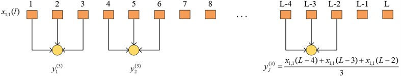
Step 1: Let the $i$-th segment signal in the sample of category $k$ be $x_{k,i}\left(l\right)$, and define the coarse-grained sequence $y_{ }^{\left(\alpha \right)}=\{y_1^{\left(\alpha \right)},y_2^{\left(\alpha \right)},\cdot \cdot \cdot ,y_j^{\left(\alpha \right)}\}$ for signal $x_{k,i}\left(l\right)$ by Eq. (1):

1

$y_j^{\left(\alpha \right)}=\frac{1}{\alpha }{\sum }_{l=(j-1)\alpha +1}^{j\alpha }{x}_{k,i}\left(l\right), 1\le j\le \frac{L}{\alpha },$

where, $y_{ }^{\left(\alpha \right)}$ represents the coarse-grained sequence under the scale factor (positive integer), and $y_j^{\left(\alpha \right)}$ represents the $j$-th point. The above processing procedure can be represented by the following Fig. 1 (taking $\alpha =\text{3}$, $k=\text{1}$, $i=\text{1}$ as examples, in the actual situation, $L\gg \alpha$, assuming the remainder of $L/\alpha$ is 2).

Fig. 1Schematic diagram of the MFSE coarse-graining sequence process

Step 2: Calculate the FSE value of the coarse-grained sequence $y_{ }^{\left(\alpha \right)}$ under the scale factor $\alpha$, and then the FSE value ($FS{E}_{\alpha }\left(x_{k,j}\right(l\left)\right)$) of signal $x_{k,i}\left(l\right)$ under the scale factor $\alpha$ can be obtained.

The feature vector $MFS{E}_{FV}\left(x_{k,j}\right(l\left)\right)$ composed of the MFSE entropy of signal $x_{k,i}\left(l\right)$ is expressed by Eq. (2):

2

$MFS{E}_{FV}\left(x_{k,i}\left(l\right)\right)=\left[FS{E}_1\left(x_{k,i}\left(l\right)\right),FS{E}_2\left(x_{k,i}\left(l\right)\right),\cdot \cdot \cdot ,FS{E}_{\alpha }\left(x_{k,i}\left(l\right)\right)\right].$

To obtain the CMFSE value, the following steps are processed for each segment of the signal:

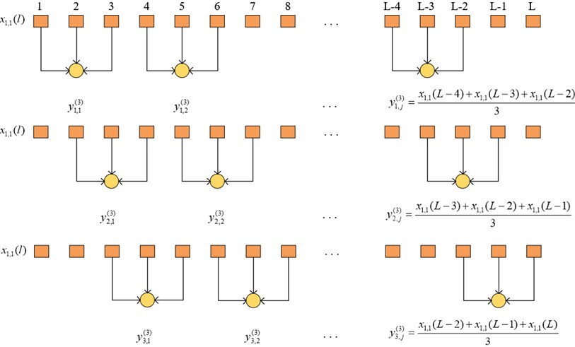
Step 1: Let the $i$-th segment signal in the sample of category $k$ be $x_{k,i}\left(l\right)$, and define the coarse-grained sequence $y_m^{\left(\alpha \right)}=\left\{y_{m,1}^{\left(\alpha \right)},y_{m,2}^{\left(\alpha \right)},\cdot \cdot \cdot ,y_{m,j}^{\left(\alpha \right)}\right\}$ for signal $x_{k,i}\left(l\right)$ by Eq. (3):

3

$y_{m,j}^{\left(\alpha \right)}=\frac{1}{\alpha }{\sum }_{l=(j-1)\alpha +m}^{j\alpha +m-1}{x}_{k,i}\left(l\right), 1\le j\le \frac{L}{\alpha }, 1\le m\le \alpha ,$

where, $y_m^{\left(\alpha \right)}$ represents the $m$-th coarse-grained sequence under the scale factor $\alpha$, and $y_{m,j}^{\left(\alpha \right)}$ represents the $j$-th point of $y_m^{\left(\alpha \right)}$. The above processing procedure can be represented by the following Fig. 2 (taking $\alpha =\text{3}$, $k=\text{1}$, $i=\text{1}$ as examples, in the actual situation, $L\gg \alpha$, assuming the remainder of $L/\alpha$ is 2).

Fig. 2Schematic diagram of the coarse-graining sequence process of CMFSE

Step 2: Calculate the FSE value ($FSE\left(y_m^{\alpha }\right)$) of each coarse-grained sequence $y_m^{\left(\alpha \right)}$ under the scale factor $\alpha$ and take the average to obtain the CMFSE value ($CMFS{E}_{\alpha }\left(x_{k,i}\right(l\left)\right)$) of signal $x_{k,i}\left(l\right)$ under the scale factor $\alpha$. The above calculation process is shown as Eq. (4):

4

$CMFS{E}_{\alpha }\left(x_{k,i}\left(l\right)\right)=\frac{1}{\alpha }{\sum }_{m=1}^{\alpha }FSE\left(y_m^{\alpha }\right).$

The feature vector $CMFS{E}_{FV}\left(x_{k,j}\right(l\left)\right)$ composed of the CMFSE of signal $x_{k,i}\left(l\right)$ is expressed by Eq. (5):

5

$CMFS{E}_{FV}\left(x_{k,i}\left(l\right)\right)=\left[CMFS{E}_1\left(x_{k,i}\left(l\right)\right),CMFS{E}_2\left(x_{k,i}\left(l\right)\right),\cdot \cdot \cdot ,CMFS{E}_{\alpha }\left(x_{k,i}\left(l\right)\right)\right].$

3. Results

3.2. Experimental results of the CWRU dataset

The first dataset used in this article is Case Western Reserve University (CWRU) laboratory bearing failure data set, the experiment platform are shown in Fig. 3. This experimental platform is composed of a motor (left), a torque sensor/encoder (middle), and a dynamometer (right). The tested bearing supports the motor shaft. The tested bearings (inner ring, outer ring, and rolling elements) have different fault diameters. The vibration data of the bearings under different rotational speeds and loads are tested by an accelerometer. The data parameters selected for study in this paper are from the bearings at the motor drive end. The sampling rate is 12 KHz and there are four working conditions (0 HP-1797 rmp, 1 HP-1772 rmp, 2 HP-1750 rmp, 3 HP-1730 rmp). This paper selects ten types of data, including normal bearing data, for classification research. Under each working condition, the specific parameters of each category of data sets and samples produced in this paper are shown in Tables 1 and 2.

Fig. 3CWRU motor bearing experimental platform [37]

The CMFSE values of each sample in the corresponding dataset in Table 2 are extracted to obtain the feature vector. The following Fig. 4 shows the comparison of CMFSE values of these ten types of faults under different scale factors (taking the first sample of each type of data under the working condition of 0 HP-1797 rmp as an example). It can be seen from Fig. 4 that with the increase of the scale factor value, the CMFSE values corresponding to different types of faults generally show a decreasing trend, the fluctuation range gradually becomes smaller, and the CMFSE values of different types of faults have a certain degree of discrimination, which is conducive to the subsequent SVM classification.

Next, the above ten types of feature vectors are sent into the SVM for classification. The parameter value corresponding to the kernel function is set to 600, and the value of the penalty parameter is set to 2. The division ratio of the training set and the test set is 1:1. The following Figs. 5-8 show the confusion matrix diagrams of the classification results under different working conditions.

Table 1Parameter settings for making the dataset (CWRU)

Parameters	Value
L	2048
M	100
Q	1000

Table 2Parameter settings for making the dataset (CWRU)

Fault diameter (inch)	Fault location	Label
0	Normal	1
0.007	Inner Race	2
0.007	Ball	3
0.007	Outer Race	4
0.014	Inner Race	5
0.014	Ball	6
0.014	Outer Race	7
0.021	Inner Race	8
0.021	Ball	9
0.021	Outer Race	10

Fig. 4CMFSE values of ten types of faults under different scale factors (0 HP-1797 rmp working conditions, the first sample of each type of data)

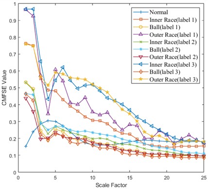
Fig. 5Confusion matrix of SVM classification results (0 HP-1797 rmp)

Fig. 6Confusion matrix of SVM classification results (1 HP-1772 rmp)

Fig. 7Confusion matrix of SVM classification results (2 HP-1750 rmp)

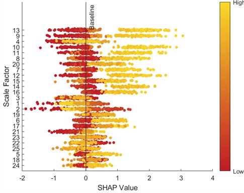
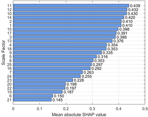
To further analyze feature contributions, the SHapley Additive exPlanations (SHAP) tool was introduced to quantify the importance of features at various scales. Specifically, this paper uses SHAP beeswarm plots and SHAP bar charts to visualize features. SHAP beeswarm plots provide a visual representation of the distribution of feature contributions to predictions. The vertical axis of the SHAP beeswarm plot represents features sorted in descending order by their global average SHAP value, with the most important feature at the top. The horizontal axis represents the range of SHAP values, with negative contributions to the left of the baseline (decreasing the predicted value) and positive contributions to the right (increasing the predicted value). A single dot represents the SHAP contribution of a sample to that feature. The color of the dot indicates the actual magnitude of the feature value. SHAP bar charts further quantify the importance of each feature, with importance decreasing from top to bottom, with the top feature having the greatest impact on the model output. Figs. 9-16 show the SHAP beeswarm plots and SHAP bar charts for the first dataset.

Fig. 8Confusion matrix of SVM classification results (3 HP-1730 rmp)

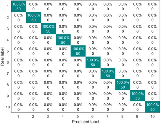
Fig. 9SHAP beeswarm plot (0 HP-1797 rmp)

In order to prove the superiority of this method, this paper compares the classification accuracy, memory usage, and running time by changing different entropy methods. The results are shown in Table 3.

Table 3Comparison of fault classification accuracy under different working conditions (CWRU)

Working condition	Entropy method	Average classification accuracy (%)	Memory usage (MB)	Run time (S)
0 HP-1797 rmp	CMFSE	100	29.9	137.9.
	MFSE	94.2	28.2	31.2
1 HP-1772 rmp	CMFSE	100	29.7	138.2.
	MFSE	96.4	27.8	30.8
2 HP-1750 rmp	CMFSE	100	30.1	137.5.
	MFSE	99.8	28..2	31.7
3 HP-1730 rmp	CMFSE	100	29.5	138.9.
	MFSE	100	28.4	31.5

Fig. 10SHAP bar chart (0 HP-1797 rmp)

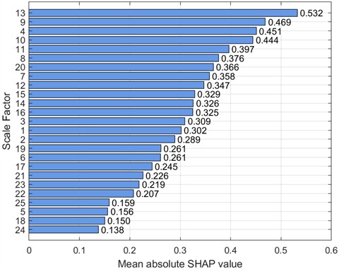
Fig. 11SHAP beeswarm plot (1 HP-1772 rmp)

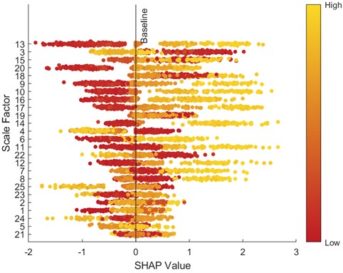
Fig. 12SHAP bar chart (1 HP-1772 rmp)

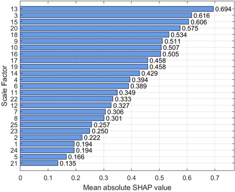
Fig. 13SHAP beeswarm plot (2 HP-1750 rmp)

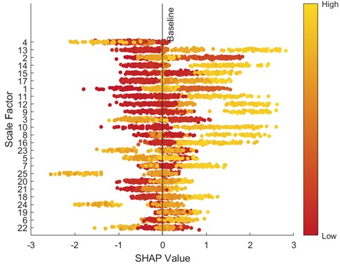
Fig. 14SHAP bar chart (2 HP-1750 rmp)

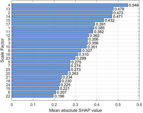
Fig. 15SHAP beeswarm plot (3 HP-1730 rmp)

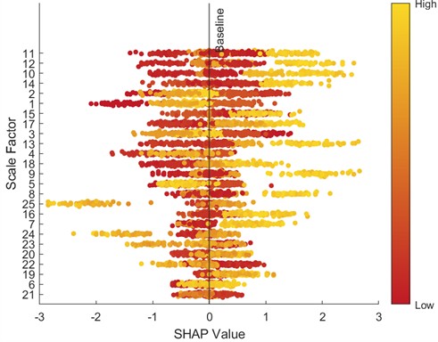
Fig. 16SHAP bar chart (3 HP-1730 rmp)

3.3. Experimental results of the SU dataset

In order to further verify the performance of the proposed method, this paper uses another dataset from Southeast University (SU) in China for verification. The experimental platform is shown in Fig. 17.

Fig. 17Electric motor experimental platform of southeast university [38]

The dataset consists of a gearbox fault dataset and a bearing fault dataset. This paper uses a bearing fault dataset, which contains two working conditions (20 Hz-0 V, 30 Hz-2 V). Each working condition contains five types of data including normal bearings. These raw data are collected by vibration sensors installed on the experimental platform. The specific parameters of each fault category sample under each working condition are shown in Table 4. The other parameter settings of this dataset are the same as those of the previous dataset, and will not be repeated in this article.

Table 4Fault sample parameter (SU)

Fault location	Label
Health working state	1
Inner ring	2
Ball	3
Outer ring	4
Combination fault (both inner ring and outer ring)	5

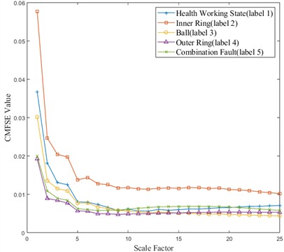
After each sample data is reconstructed, the CMFSE value is extracted to obtain the feature vector. Fig. 18 shows the comparison of CMFSE values of these five types of faults under different scale factors (taking the first sample of each type of data under the working condition of 20 Hz-0 V as an example). It can be seen from Fig. 18 that with the increase of the scale factor value, the CMFSE values corresponding to different types of faults generally show a decreasing trend, the fluctuation range gradually becomes smaller, and the CMFSE values of different types of faults have a certain degree of discrimination, which is conducive to the subsequent SVM classification.

Fig. 18CMFSE values of five types of faults under different scale factors (20 Hz-0 V working condition, the first sample of each type of data)

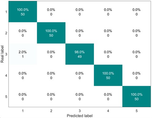
Next, the feature vectors composed of the above five types of faults are sent into the SVM for classification. The following Fig. 19 and Fig. 20 show the classification result graphs under different working conditions.

Fig. 19Confusion matrix of SVM classification results (20 Hz-0 V)

The following Figs. 21 to 24 are the corresponding SHAP beeswarm plots and SHAP bar charts.

Fig. 20Confusion matrix of SVM classification results (30 Hz-2 V)

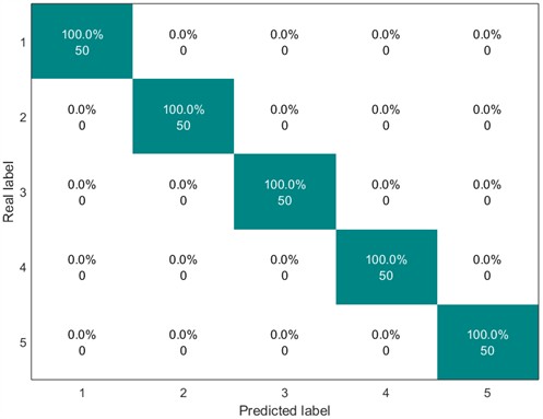
Fig. 21SHAP beeswarm plot (20 Hz-0 V)

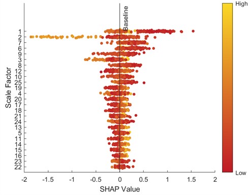
Fig. 22SHAP bar chart (20 Hz-0 V)

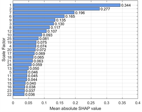
Fig. 23SHAP beeswarm plot (30 Hz-2 V)

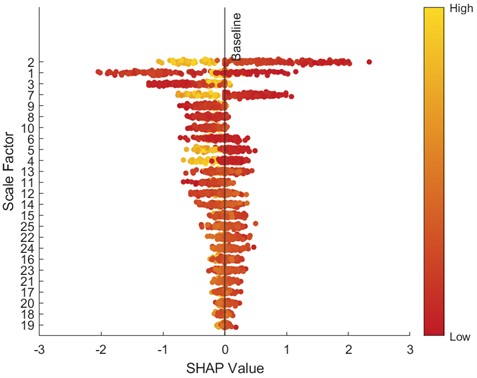
Fig. 24SHAP bar chart (30 Hz-2 V)

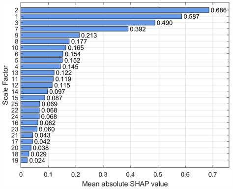
Table 5 compares the classification accuracy, space occupied, and running time of two different entropy methods.

Table 5Comparison of fault classification accuracy under different working conditions (SU)

Working condition	Entropy method	Average classification accuracy (%)	Memory usage (MB)	Run time (S)
20 Hz-0 V	CMFSE	99.6	12.5	68.8
	MFSE	98.	11.6	15.4
30 Hz-2 V	CMFSE	100	12.9	69.1
	MFSE	96	11.8	15.2

4. Discussions

It can be known from Figs. 5 to 8 that the classification accuracy of the CMFSE method under the four working conditions in the first dataset is 100 %. However, the classification accuracy of the MFSE method is 100 % only under the fourth working condition, and the classification accuracy is lower than 100 % under other working conditions. The average accuracy of the MFSE method under all working conditions is 97.6 %, and the CMFSE method is 2.4 % higher than the MFSE method. This result proves the superiority of the method proposed in this paper.

It can be known from Figs. 19 to 20 that the average classification accuracy of the CMFSE method under the two working conditions in the second dataset is 99.8 %, while the average classification accuracy of the MFSE method under the two working conditions in the second dataset is 97 %. The CMFSE method is 2.8 % higher than the MFSE method. This further proves the superiority of the method proposed in this paper.

In terms of algorithm complexity, in terms of space complexity, it can be seen from Table 3 that the CMFSE method occupies an average memory space of 29.8 MB, and the MFSE method occupies an average memory space of 28.2 MB, and the difference between the two is not large. In terms of time complexity, it can be seen from Table 3 that for feature extraction and classification of 1000 samples, the CMFSE method has an average running time of 138.1 S in four working conditions, and an average time of about 0.14 S per sample. The MFSE method has an average running time of 31.3 S in four working conditions, and an average time of about 0.03 S per sample. The MFSE method takes less time. Table 5 shows that for feature extraction and classification of 500 samples, the CMFSE method uses an average memory footprint of 12.7 MB, while the MFSE method uses an average memory footprint of 11.7 MB, a significant difference between the two methods. Table 5 also shows that the CMFSE method has an average runtime of 68.9 S in both conditions, with an average runtime of approximately 0.14 S per sample. The MFSE method has an average runtime of 15.3 S in both conditions, with an average runtime of approximately 0.03 S per sample, resulting in a shorter runtime. Overall, the CMFSE method has a higher complexity than the MFSE method, but its classification accuracy is superior. Considering the similar memory footprint between the two methods, the CMFSE method takes less than 0.2 S to diagnose a single sample, which still demonstrates good real-time performance in practical applications.

Furthermore, this paper only requires half of the samples in the dataset to participate in the training, and a very high classification accuracy can be achieved on the test set, indicating that the method proposed in this paper has a strong feature extraction ability. However, there is still room for further optimization of the method proposed in this paper. For example, we can study the influence of the sample data length of the dataset and the number of features in the feature vector on the fault diagnosis accuracy, so as to find a balance between the algorithm complexity and the diagnosis and classification accuracy. We can also further study the combination of the proposed method and convolutional neural network for fault classification.

5. Conclusions

The composite multi-scale fuzzy slope entropy method proposed in this paper does not need to decompose the original signal before extracting the rolling bearing fault features, but directly extracts the entropy value of the original signal, which is conducive to reducing the complexity of the algorithm. At the same time, the method proposed in this paper has been verified on two public data sets and has the advantage of high classification accuracy. Compared with the multi-scale fuzzy slope entropy, this method has better fault classification performance and can be used in the field of motor rolling bearing fault diagnosis, which has certain practical application value.