Abstract
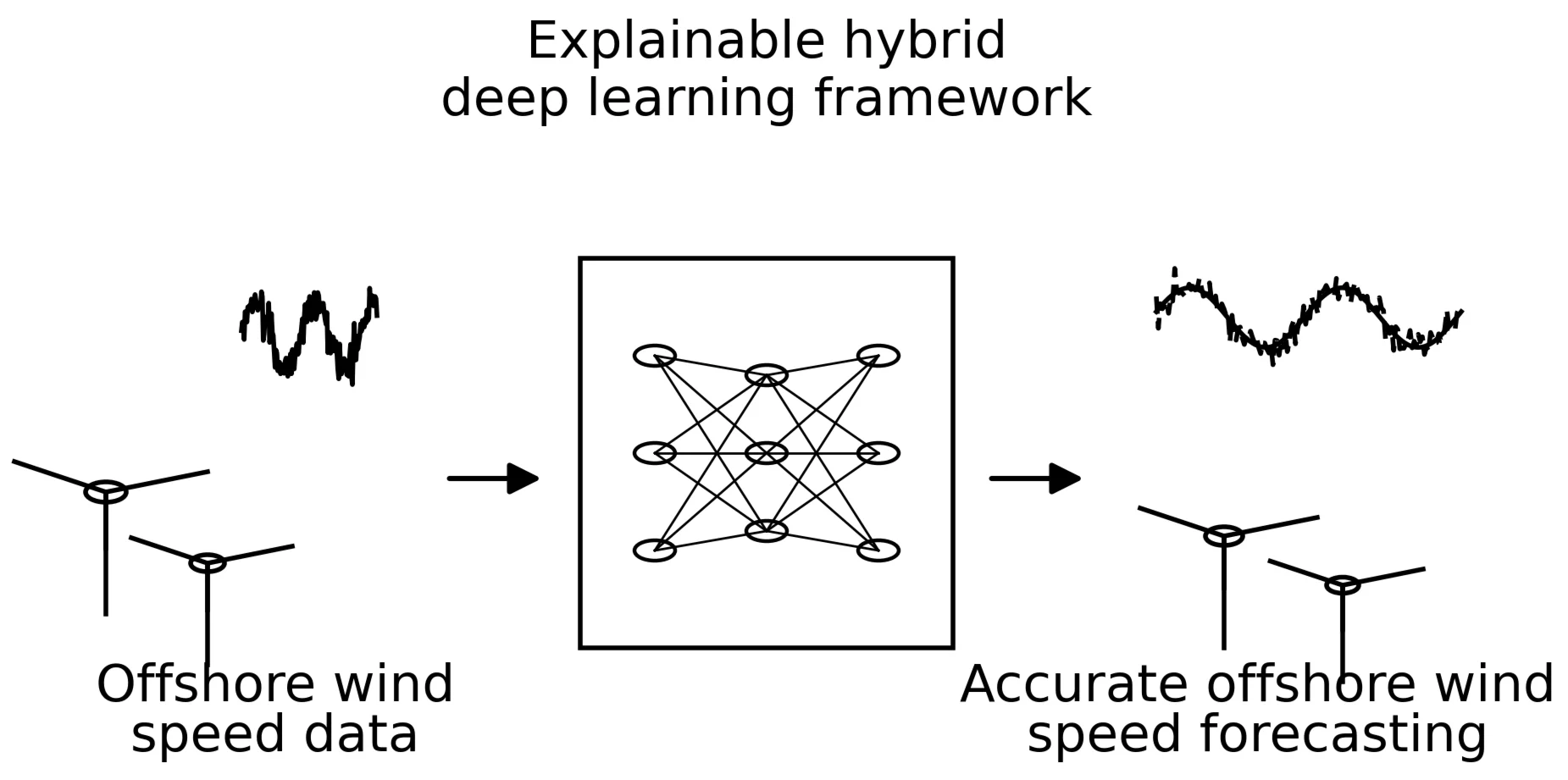
Interpretability has become a critical requirement in modern deep learning applications for renewable energy forecasting, especially in complex and safety-critical contexts such as offshore wind power systems. To simultaneously improve predictive accuracy and model transparency, this study proposes an explainable hybrid deep learning framework – VFE-IVYA-CNN-BiGRU – for offshore wind speed forecasting. The model begins with feature selection via Pearson Correlation (PCs) to identify the most relevant meteorological variables from a full set of candidates, thereby enhancing input quality and reducing redundancy. The selected features are then passed through a robust preprocessing module (VFE), which integrates Variational Mode Decomposition (VMD) and Fuzzy Entropy (FE). VMD decomposes the original wind speed sequence into intrinsic mode functions (IMFs), capturing multi-scale temporal structures, while FE quantifies the complexity of each IMF to filter out noise-dominated components. The reconstructed sub-sequences are first processed through a Convolutional Neural Network (CNN) to capture temporal local dependencies, and then passed into a Bidirectional Gated Recurrent Unit (BiGRU), which effectively learns time dependencies in both forward and backward directions. To further enhance model performance, the Ivy Algorithm (IVYA) is employed to optimize hyperparameters adaptively, improving convergence and generalization. To improve interpretability, SHapley Additive exPlanations (SHAP) are utilized to quantify the contribution of each meteorological feature to the model's output, revealing both dominant drivers (e.g., gust speed) and interaction patterns across seasons. The proposed framework is evaluated using seasonal offshore wind datasets (spring, summer, autumn, and winter) sourced from a wind power site along the Guangdong coastline, China, and contrasted with six leading benchmark models. Empirical findings reveal that the proposed VFE-IVYA-CNN-BiGRU consistently outperforms existing methods in terms of accuracy, robustness, and interpretability. The integration of SHAP-based explanations ensures model transparency, making the approach a reliable tool for intelligent control and decision support in offshore wind farm operations.
Highlights
- An explainable hybrid deep learning framework is proposed for offshore wind speed forecasting.
- The framework integrates signal decomposition and deep neural networks to enhance prediction accuracy.
- Explainable analysis is conducted to reveal the contributions of key meteorological factors.
1. Introduction
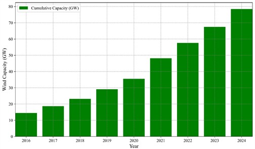
With the continuous depletion of fossil fuel resources and the growing environmental pressures associated with their use, the development of clean and sustainable energy has become a global priority. Among various renewable options, offshore wind power has attracted significant attention due to its abundant installation space, greater wind stability, and larger turbine capacity. In China, it plays a central role in the national strategy of “integrating land-sea development and accelerating marine power construction” [1-3]. According to the Global Wind Energy Council (GWEC), global offshore wind capacity reached 78.52 GW by the end of 2024 and is expected to rise to 380 GW by 2030 [4].
Despite its rapid growth, large-scale grid integration of offshore wind remains challenging because wind speed exhibits strong variability, intermittency, and nonlinear behavior. Accurate short-term forecasting is therefore crucial for secure grid operation, economic dispatch, and efficient utilization of wind resources. Generally, forecasting tasks are categorized into short-, medium-, and long-term horizons, among which high-precision short-term forecasting is particularly vital for real-time operation and control [5, 6].
Fig. 1Global cumulative installed offshore wind capacity (GW)
Over the past decades, numerous techniques have been proposed to forecast wind speed, which are typically categorized into three main groups: physics-based models, statistical methods, and data-driven approaches. Physics-based models, particularly numerical weather prediction (NWP), are based on the equations of atmospheric dynamics and thermodynamics. These models simulate wind behavior by solving partial differential equations under defined boundary and initial conditions. Although NWP models offer high spatiotemporal resolution and theoretical rigor, they require significant computational resources and are highly sensitive to initialization errors, rendering them less suitable for ultra-short-term forecasting tasks where timeliness and adaptability are critical [7, 8].
Statistical methods, such as autoregressive (AR), moving average (MA), and their extended versions including ARMA and ARIMA, model wind speed as linear time series [9-11]. These models are computationally efficient and easy to interpret but inherently limited in capturing the nonlinear and nonstationary characteristics of wind speed data. Hybrid extensions such as ARIMA-GARCH have been proposed to incorporate volatility modeling, yet they still struggle with the multiscale fluctuations observed in real-world wind speed series.
To overcome these constraints, machine learning (ML) methods have emerged as attractive alternatives, owing to their capability to capture intricate nonlinear patterns without the need for predefined physical formulations. Techniques like support vector machines (SVM) [12], extreme learning machines (ELM) [13], Artificial Neural Network (ANN) [14], Naive Bayes model and random forests (RF) [15] have shown promising results in wind speed prediction, outperforming traditional statistical approaches in terms of prediction accuracy. However, shallow ML models generally require feature engineering and may not generalize well in high-dimensional or highly volatile environments. Their inability to learn hierarchical representations from raw data constrains their forecasting robustness, particularly under multiscale and nonstationary conditions [16].
In recent developments, deep learning has gained prominence in time series forecasting, owing to its ability to perform hierarchical feature representation and enable end-to-end model training. Deep neural networks (DNN), convolutional neural networks (CNN), Generative Adversarial Network (GAN), long short-term memory (LSTM), and gated recurrent units (GRU) have found extensive application in forecasting tasks related to wind speed and wind power.
CNNs are effective at extracting local patterns and temporal correlations, while RNNs and their variants capture sequential dependencies. Among them, GRU and its bidirectional version (BiGRU) are particularly suitable for wind time series modeling, offering a balance between model complexity and temporal representation power. Compared to LSTM, BiGRU employs fewer parameters and demonstrates faster convergence with comparable forecasting accuracy, making it a competitive choice for real-time and large-scale applications [17-23].
Despite their strengths, deep learning models often face challenges in learning from raw wind speed sequences due to their high-frequency oscillations, seasonal heterogeneity, and embedded noise. To mitigate this issue, signal decomposition techniques are frequently introduced as a preprocessing step to improve signal smoothness and regularity. Wavelet transform (WT) [24], empirical mode decomposition (EMD) [25, 26], Ensemble Empirical Mode Decomposition (EEMD) and variational mode decomposition (VMD) [27] are among the most widely used methods in this context. WT provides multiresolution analysis but requires a predefined mother wavelet, potentially limiting adaptability. EMD and EEMD is capable of adaptively extracting intrinsic mode functions (IMFs); nevertheless, traditional methods are susceptible to problems like mode mixing and edge distortion. In contrast, Variational Mode Decomposition (VMD) reframes the decomposition task as a constrained optimization framework based on variational methods and generates band-limited IMFs with better mode separation and noise suppression capabilities, thereby enhancing signal interpretability and downstream model learnability [28, 29].
To further enhance the quality of decomposed components, entropy-based complexity measures such as approximate entropy (AE) [30], permutation entropy (PE) and sample entropy (SE) [31], and fuzzy entropy (FE) [32, 33] have been adopted. These methods evaluate the irregularity and unpredictability of time series components, aiding in the selection of informative IMFs. Compared with AE and SE, FE demonstrates superior robustness to noise and sensitivity to subtle variations. By reconstructing subsequences based on FE similarity, redundant or low-information components can be filtered out, improving model efficiency and generalization while retaining essential dynamic characteristics.
In parallel, the performance of deep neural networks is heavily influenced by hyperparameter configurations such as learning rate, batch size, number of layers, and hidden units. Manual tuning is time-consuming and prone to suboptimal configurations. To address this, metaheuristic optimization algorithms have been introduced, including genetic algorithms (GA) [34], particle swarm optimization (PSO) [35], gray wolf optimizer (GWO) [36], and more recently, the ivy algorithm (IVYA) [37]. Inspired by biological behavior of ivy plants, IVYA balances exploration and exploitation by modeling population evolution through coordinated propagation and light-seeking strategies. Empirical studies have shown that IVYA achieves faster convergence and better global optimization capability than traditional heuristics, making it well-suited for complex neural network hyperparameter tuning.
While improving forecasting accuracy remains a central objective, recent research has increasingly emphasized the interpretability of predictive models, particularly in energy forecasting scenarios where decisions must remain transparent and trustworthy. Despite their strong predictive capability, deep learning models are often criticized as “black boxes,” motivating the adoption of explainable artificial intelligence (XAI) techniques. Among them, SHAP provides a unified, game-theoretic framework for quantifying feature contributions at both global and instance levels, offering insights into the meteorological drivers of forecast outcomes and their seasonal interactions [38, 39].
Recent progress in signal decomposition, deep learning architectures, optimization algorithms, and interpretability tools has markedly improved wind speed forecasting performance. Nevertheless, combining these advances into a single framework that achieves both high accuracy and interpretability remains challenging. To address this gap, this paper proposes an explainable hybrid model for offshore wind speed prediction that integrates signal decomposition and filtering, deep sequence modeling, automated hyperparameter tuning, and SHAP-based interpretability.
The model is evaluated using offshore wind datasets from Guangdong, China, across four seasons and compared with six advanced baselines. Experimental results demonstrate significant gains in forecasting accuracy and model transparency.
The main contributions of this work are summarized as follows:
(1) A correlation-based feature selection strategy is employed to extract nine dominant meteorological variables, reducing input dimensionality and improving learning efficiency.
(2) A VFE module is designed to decompose wind speed signals and retain components with higher complexity and predictive value, alleviating nonlinearity and noise.
(3) A CNN-BiGRU hybrid network is constructed to jointly capture local temporal features and bidirectional dependencies, enabling robust sequence representation.
(4) The Ivy Algorithm (IVYA) is adopted for automated hyperparameter tuning, enhancing convergence speed and predictive stability.
(5) SHAP is used to interpret the contribution of each meteorological feature, providing both global and local insights into the model’s decision-making process.
2. Methods
2.1. VMD and fuzzy entropy-based signal processing
To capture the complex, non-stationary, and nonlinear characteristics present in offshore wind speed data, this study adopts a two-stage preprocessing technique combining Variational Mode Decomposition (VMD) and Fuzzy Entropy (FE), hereafter referred to as VFE.
By applying VMD, intrinsic mode function (IMF) can be derived from the original wind speed signal through adaptive decomposition, each with compact bandwidth around an adaptive center frequency . To achieve accurate signal reconstruction, the variational formulation Eq. (1) aims to constrain the overall bandwidth of the extracted modes as much as possible [40]:
where, is the time derivative, denotes convolution, and is Dirac function. To address this optimization task under constraints, a Lagrange multiplier and penalty term are introduced, yielding the augmented Lagrangian:
The decomposition quality being highly sensitive to the penalty factor and mode number : inappropriate settings may lead to under- or over-decomposition, impacting model performance.
After decomposition, FE is employed to evaluate the complexity of each IMF. Unlike sample entropy, FE uses an exponential membership function to quantify the similarity between phase space vectors [41]. Given a time series , the fuzzy similarity is defined as Eq. (3):
where is the Chebyshev distance, is the similarity tolerance, and is the fuzzy power. The FE is computed by comparing the average similarity of vectors of dimension and :
A higher FE value indicates greater irregularity and complexity. In this work, IMFs with higher FE are retained for prediction, while low-entropy components are discarded to reduce noise and computation burden.
By combining the adaptive decomposition capability of VMD and the complexity filtering power of FE, the VFE module enhances the signal quality and preserves meaningful temporal features for downstream prediction.
2.2. Ivy algorithm (IVYA)
Inspired by the adaptive growth and climbing patterns of ivy plants, the Ivy Algorithm (IVYA) was introduced as a meta-heuristic optimization strategy by Ghasemi et al. (2024) [42]. By simulating the biological mechanisms of ivy propagation – including coordinated expansion, adaptive search, and competition for sunlight – IVYA offers an effective strategy for solving complex, high-dimensional optimization problems.
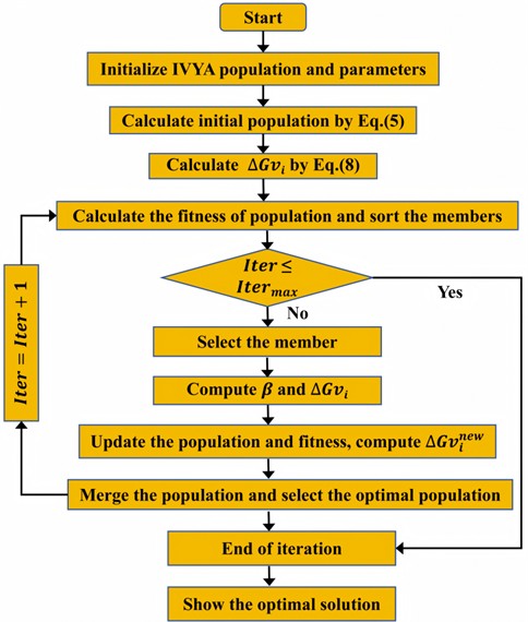
IVYA models the ivy’s growth process using discrete-time dynamic equations and evolutionary rules. Its optimization framework consists of five major stages: (1) population initialization, (2) coordinated growth, (3) light-seeking movement, (4) expansion and adaptation, and (5) survivor selection. These components work together to guide the population toward global optima through both exploration and exploitation mechanisms. The IVYA’s process flow is depicted in Fig. 2.
Population initialization. Eq. (5) is employed to initialize the IVYA population with random positions distributed throughout the search space:
where, a vector with dimension of uniformly distributed random numbers is represented by . is the number of populations.
Coordinated growth. It is postulated that the growth rate of ivy plants varies as a function of time. Drawing upon extensive experimental data, a corresponding difference equation describing the growth rate of individual members is derived:
where the vectors and represent the growth rate of a discrete-time system, denotes a uniformly distributed real number within the range [0, 1], while indicates a normally distributed random vector of dimension .
Light-seeking movement. Young ivy is often guided to grow toward nearby trees or established ivy that has secured a support structure, allowing access to sunlight and promoting population sustainability.
The Eq. (7-8) describes how Ivy uses to move logically in the direction of the radiant source:
Expansion and adaptation. Following a global search, member locates the closest and most influential neighbor within the solution space, and tries to follow the best member of the population to find the best candidate solution. This phase is represented by the Eq. (9):
Fig. 2Flowchart of the IVYA
Eq. (10) is applied to compute the present growth rate of member , (which is exactly similar to the formula used to calculate ):
Survivor selection. In order to simulate the alternating stages, namely “climb” and “expand”, the method is used. If the objective value for member falls below the product of and parameter , Eq. (7) is used to expand the branch and leaf width of the ivy tree. Otherwise, the upward growth and climbing behavior of the ivy is guided by Eq. (9).
2.3. Convolutional neural network (CNN)
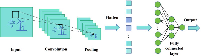
Due to their effectiveness in capturing local temporal patterns from structured inputs, Convolutional Neural Networks (CNNs) have become a prevalent choice for feature extraction tasks. The CNN architecture typically consists of three primary layers: the input layer, a series of hidden layers (including convolution and pooling operations), and the output layer [43, 44]. The CNN’s structure is shown as Fig. 3.
The core component of a CNN is its convolutional layer, which utilizes learnable filters to derive significant local characteristics from the input. This process is mathematically described in Eq. (11):
where denotes the feature map fed from the preceding layer, is convolutional kernel, is the bias term, denotes convolution operation, is the nonlinear activation function (commonly ReLU).
Following convolution, a pooling layer – specifically, max pooling – is applied to reduce dimensionality and suppress noise, preserving dominant features while mitigating overfitting. The pooling operation is defined as:
where represents the pooling function applied to the output feature map.
The final layer is typically fully connected, which aggregates extracted features and maps them to the target prediction.
This study uses CNN primarily to capture short-term temporal dependencies in preprocessed wind speed components, providing an effective input representation for subsequent temporal modeling.
Fig. 3Architecture of the CNN
2.4. Bidirectional gated recurrent unit (BiGRU)
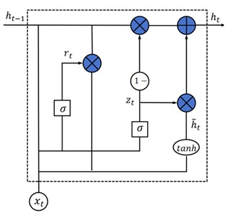
To effectively model temporal relationships in sequential data, the BiGRU is employed. Compared to LSTM, the GRU architecture achieves similar performance while simplifying the gating mechanism by using fewer components [45, 46]. Its structure revolves around two essential components – the reset and update gates – which are visualized in Fig. 4(a).
The mathematical formulation of a GRU unit is as follows:
Eqs. (13-16) are related to each other and cannot be used alone. is reset gate. is update gate. is candidate hidden layer state, reflecting the input information. is the output of the hidden layer. and are the Sigmoid function and activation function, respectively; , , , , , are all training parameter matrices.
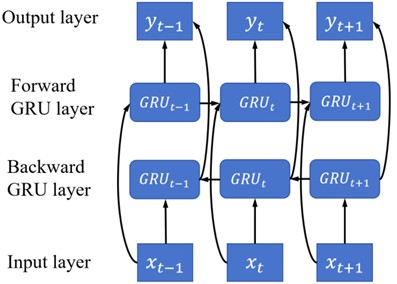
BiGRU extends the GRU by processing the input sequence in both forward and backward directions, capturing richer temporal dependencies. As shown in Fig. 4(b), it consists of two parallel GRUs: one traversing the sequence from past to future, the other in reverse.
The output at time is computed as:
where and are the forward and backward hidden states, , are the corresponding output weights, is the bias term.
Compared with LSTM, BiGRU offers similar accuracy with fewer parameters and faster training convergence, thereby rendering it suitable for applications involving real-time forecasting. In this work, BiGRU is employed after CNN to model both forward- and backward-influenced temporal patterns in the offshore wind speed sequence, enhancing prediction robustness.
Fig. 4Architectures of a) GRU and b) BiGRU
a)
b)
2.5. SHAP Theory
SHAP (SHapley Additive exPlanations) is an explainable AI method based on cooperative game theory, designed to quantify the impact of each feature input on the prediction results produced by the model. It attributes the prediction of a model to the sum of feature contributions, where each feature’s effect is measured by its Shapley value [47, 48].
For a given instance , the model output is defined using Eq. (18):
where represents the expected output over the entire dataset, and denotes the marginal contribution of the th feature.
The Shapley value of feature is defined as Eq. (19):
In this context, is the complete set of the features, while refers to a subset of that excludes the specific feature . The represents the model’s output based solely on the features contained in .
This formula computes the average marginal contribution of feature over all possible subsets , ensuring fairness and consistency in feature attribution. In practical implementation, SHAP approximates these values through sampling and model-specific explainers, such as TreeSHAP or KernelSHAP.
The key advantages of SHAP lie in its solid theoretical foundation and practical utility. It ensures consistency, meaning that if a feature has a greater impact on the output, its SHAP value will not be lower than that of a less influential feature. SHAP also provides local accuracy by ensuring that the sum of all feature attributions equals the difference between the model prediction and the expected output. Furthermore, by aggregating individual explanations across multiple instances, SHAP enables global interpretability, offering insights into overall feature importance and interaction effects, which is valuable for high-stakes applications like wind power forecasting.
3. Forecasting framework construction
3.1. Architecture of the CNN-BiGRU network
The CNN model alternates between convolutional and pooling layers, utilizing local connectivity and weight sharing to efficiently extract temporal features from the original signal. This process enables the network to automatically learn local patterns and form a dense, informative feature representation. Given its ability for automatic feature extraction and compatibility with sequential data, CNN is applied to capture temporal dependencies in offshore wind speed time series.
In the BiGRU component, the input data is processed bidirectionally using Gated Recurrent Units (GRUs). This allows the network to get temporal dependencies from both future and past contexts, enhancing its capacity to model the entire sequence structure. The reuse of weights across time steps enhances model expressiveness without increasing the number of parameters, which helps mitigate underfitting. Considering the volatility and uncertainty of offshore wind speed, combining CNN and BiGRU allows the model to achieve both efficient feature extraction and effective temporal modeling. The structure of the CNN-BiGRU model is illustrated in Fig. 5. The structure can be described as follows:
Input Layer: The input is structured as a two-dimensional matrix of size, where corresponds to the temporal dimension of the sequence, and indicates the feature dimensionality per time step. The CNN module first processes this data to extract temporal patterns.
Convolutional Layer: 1D convolutional layers are used to extract temporal features. Each has a kernel size of 2 with a stride of 1, and the number of filters is set to 32 and 64 respectively. ReLU is used as the activation function, introducing non-linearity and accelerating convergence by zeroing out negative activations.
Pooling Layer: A max-pooling layer follows each convolutional layer to reduce dimensionality and eliminate less informative features. The pooling size is 2×1 with a stride of 2. The output of the pooling layers is flattened into a time sequence format suitable for BiGRU processing.
BiGRU Layer: The extracted features are then input into the BiGRU network, which processes the sequence bidirectionally to capture comprehensive temporal dependencies. A Dropout layer is added within the BiGRU to prevent overfitting by randomly deactivating some units during training. The final output is passed through a fully connected layer to generate the predicted wind speed.
Optimization and Training: The Adam optimizer is employed for training due to its adaptive learning rate capabilities. The number of training epochs is set between 1 and 200, and the initial learning rate ranges from 0.001 to 0.01. A learning rate decay factor of 0.1 is applied to ensure stable convergence. The configurations are chosen to achieve a trade-off between training speed and the model’s ability to generalize.
The specific configurations of the CNN-BiGRU model, including convolutional kernel sizes, number of filters, dropout rate, and optimization settings, are detailed in Table 1. These settings are based on standard practices in deep learning for time series modeling and have been refined to ensure effective temporal feature extraction, training stability, and model generalization. Particular attention has been paid to adapting the convolution and pooling parameters to the 1D structure of time series data, as well as to selecting appropriate ranges for hyperparameter tuning.
Fig. 5Architecture of the CNN-BiGRU
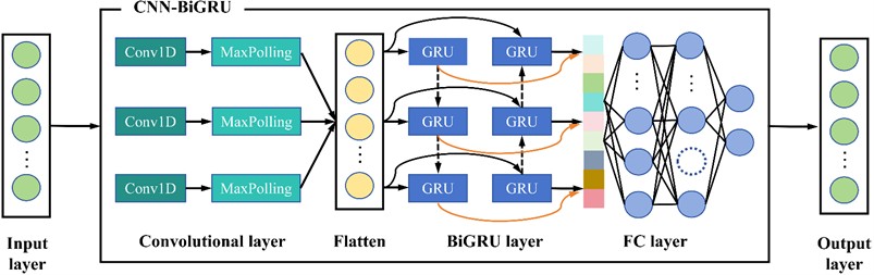
Table 1Hyperparameter configurations of the proposed model
Module | Parameter | Value / Search range |
CNN | Number of convolutional layers | 2 |
Number of filters (per layer) | [32, 64] | |
Filter size | 3×1 | |
Activation function | ReLU | |
Number of pooling layers | 2 | |
Pooling type | Max pooling | |
Pooling kernel size | 2 × 1 | |
Pooling stride | 2 | |
Padding | Same | |
BiGRU | Number of BiGRU layers | 1 (bidirectional) |
Number of hidden units | [32, 200] | |
Dropout rate | 0.2 | |
Batch size | [8, 64] | |
Learning rate | [0.001, 0.01] | |
Learning rate decay factor | 0.1 | |
Activation function (hidden state) | Tanh | |
Optimizer | Adam | |
Loss function | Mean Squared Error (MSE) | |
Number of epochs | 100 | |
IVYA | Population size | 10 |
Maximum number of iterations | 30 | |
Optimization dimension | 4 (convolutional filters, learning rate, batch size, and number of hidden units) | |
Fitness function | Validation RMSE |
3.2. Forecasting model formulation
The modeling process of the proposed VFE-IVYA-CNN-BiGRU framework for offshore wind speed forecasting consists of three main stages, as illustrated in Fig. 6. The steps are detailed as follows:
(1) Data Acquisition and Preprocessing.
Historical offshore wind speed data are collected on a daily basis. The raw dataset is first cleaned by removing zero-value records and interpolating missing entries [49]. To avoid information leakage, the dataset is then chronologically partitioned into training and testing subsets, after which all preprocessing procedures are performed. Subsequently, min-max normalization is fitted on the training subset, and the learned scaling parameters are applied to the testing data to ensure proper time-ordered validation, as shown in Eq. (20):
where denotes the original data; and represent the maximum and minimum values of , respectively, while refers to the normalized result after transformation.
In addition to normalization, Pearson Correlation (PCs) is used to measure linear relationships among features. This step assists in filtering relevant meteorological variables before entering the VFE module while minimizing the risk of collinearity-driven leakage across target-related predictors.
Fig. 6Flowchart of the proposed VFE-IVYA-CNN-BiGRU framework
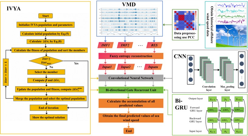
(2) Signal Decomposition and Feature Processing.
Step 2.1: For the training subset, the normalized wind speed series is decomposed using the VFE module, which combines VMD and FE. VMD adaptively separates the signal into several IMFs, each capturing specific frequency content and a residual (RES), helping to reduce signal non-stationarity. The decomposition parameters derived from the training set are then applied to process the testing subset to ensure consistency and prevent data leakage.
Step 2.2: FE is computed for each IMF component in the training subset to assess its complexity. Based on the entropy values, IMFs are reconstructed to form a new sequence that emphasizes informative structures and suppresses noise-dominated components. The reconstruction scheme is applied consistently to the testing subset using the thresholds determined from the training data.
Step 2.3: CNN is employed to extract localized temporal features, producing a high-dimensional feature matrix. This matrix is then input into the BiGRU layer to capture temporal dependencies from both forward and backward directions.
(3) Model Training and Prediction.
Step 3.1: Key hyperparameters of the CNN-BiGRU architecture are optimized using the Ivy Algorithm (IVYA), including the number of convolutional filters, learning rate, batch size, and number of hidden units.
Step 3.2: With the optimized hyperparameters, the feature-enriched dataset is used to train the CNN-BiGRU architecture. The trained model is then used to predict wind speed values on the test set. Each reconstructed component is predicted independently.
Step 3.3: Finally, the predicted sub-sequences are aggregated and then inverse normalized to restore the original scaleto yield the complete offshore wind speed forecast. The model performance is evaluated using standard error metrics, and results are compared against benchmark models.
3.3. Evaluation metrics
To assess how closely the VFE-IVYA-CNN-BiGRU model’s predictions align with actual wind speed values, this study applies four commonly used evaluation metrics: R², RMSE, MAE, and MAPE [50]. These indicators help in analyzing the predictive reliability and error magnitude of the model. The expression is shown as Eq. (21-24):
where is the true value of the th sample; is the predicted value of the th sample; is the average of all the samples; represents the number of predicted samples.
4. Case study and results
4.1. Dataset description
This study employs data collected from an offshore wind farm in Guangdong Province, China, during the one-year period spanning from the beginning to the end of 2022 (January 1 to December 31). Wind speed and associated meteorological variables were recorded at 30-minute intervals, forming the basis for seasonal prediction analysis. The dataset includes ten meteorological factors: wind direction (WDIR), gust speed (GSP), wave height (WVHT), dew point temperature (DPT), dominant wave period (DWP), sea level pressure (SLPR), air temperature (ATMP), sea surface temperature (SST), average wave period (AWP), and actual wind speed (AWS).
For seasonal evaluation, the full-year dataset is divided into four subsets corresponding to distinct time frames: Winter (January 1-31), Spring (April 1-30), Summer (July 1-31), Autumn (October 1-31). Each seasonal subset is further split into training (70 %) and testing (30 %) sets. The number of samples per season varies slightly due to the differing lengths of each month: 1488 (Winter), 1436 (Spring), 1474 (Summer), and 1484 (Autumn). Data preprocessing includes zero-value removal, interpolation for missing values, and min-max normalization.
The seasonal variations in offshore wind speed are illustrated in Fig. 7, where the temporal trends across the four seasons show distinct fluctuations and amplitudes, reflecting meteorological seasonality and variability. Table 2 provides a statistical overview of wind speed across different seasons, reporting values such as the mean, median, range (maximum and minimum), standard deviation, skewness, and kurtosis.
All experiments were conducted using a computing platform operating under Windows 11, powered by an Intel Core i9-12900H CPU and supported with 16 GB of RAM. The implementation of the model was carried out using Python 3.10, with TensorFlow 2.14 serving as the underlying deep neural modeling toolkit. All baseline and proposed models were trained under identical training budgets, input window sizes, batch settings, optimizer schedules, and stopping criteria to ensure a fair comparison. Computational metrics such as convergence curves and latency are not included to maintain focus on forecasting performance and interpretability.
Fig. 7Original offshore wind speed data in four seasons
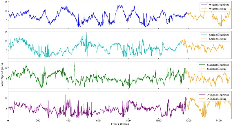
Table 2Statistical descriptions of seasonal wind speed datasets
Data set | Data length | Max | Min | Median | Mean | Std-Dev | Kurtosis | Skewness | |
Winter | All (m/s) | 1488 | 14.7 | 0.89 | 7.1 | 7.075 | 2.623 | –0.145 | 0.194 |
Training (m/s) | 1041 | 13.3 | 0.89 | 6.9 | 6.941 | 2.670 | –0.562 | 0.078 | |
Testing (m/s) | 447 | 14.7 | 1.4 | 7.2 | 7.388 | 2.483 | 0.858 | 0.592 | |
Spring | All (m/s) | 1436 | 14.8 | 0.94 | 6.3 | 6.241 | 2.333 | –0.343 | 0.113 |
Training (m/s) | 1005 | 14.8 | 0.94 | 6.0 | 6.106 | 2.576 | –0.649 | 0.213 | |
Testing (m/s) | 431 | 10.9 | 1.7 | 6.5 | 6.557 | 1.585 | 0.465 | 0.038 | |
Summer | All (m/s) | 1474 | 12.4 | 1.1 | 5.3 | 5.480 | 1.817 | –0.011 | 0.268 |
Training (m/s) | 1031 | 12.4 | 1.1 | 5.3 | 5.450 | 1.869 | 0.107 | 0.357 | |
Testing (m/s) | 443 | 9.8 | 1.4 | 5.5 | 5.550 | 1.687 | –0.459 | 0.012 | |
Autumn | All (m/s) | 1484 | 12.5 | 1.15 | 5.1 | 5.286 | 2.178 | –0.307 | 0.368 |
Training (m/s) | 1038 | 11.4 | 1.15 | 4.8 | 4.720 | 1.730 | –0.160 | 0.161 | |
Testing (m/s) | 446 | 12.5 | 1.36 | 6.8 | 6.602 | 2.518 | –0.829 | –0.273 | |
4.2. Meteorological feature analysis
Offshore wind speed is influenced by nine marine meteorological parameters, including WDIR, GSP, WVHT, DWP, AWP, SLPR, ATMP, SST and DPT. To quantitatively assess the relationships between these factors and wind speed, Pearson Correlation (PCs) analysis is employed.
The PCs between each meteorological variable and the actual offshore wind speed is calculated by Eq. (25):
where the correlation coefficient ranges from [–1, 1], when it is greater than 0, the stronger the correlation, the larger the value; is the total number of dataset; is the meteorological factor data; is the offshore wind speed data [51].
Fig. 8Feature correlation heatmap (Winter)
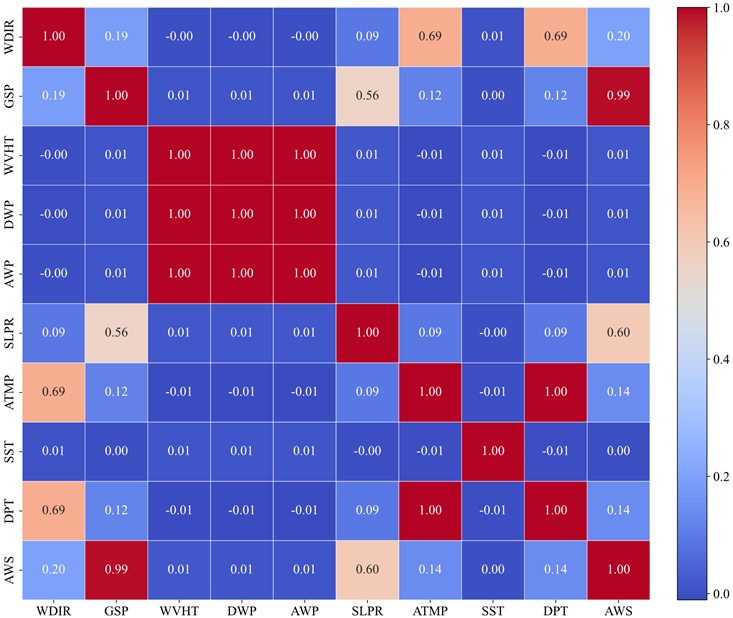
The correlation heatmap of the winter dataset is visualized in Fig. 8, clearly showing that gust speed (GSP) exhibits the highest positive correlation with wind speed, followed by SLPR and DPT. To generalize this analysis, Table 3 presents the PCs values between wind speed and all nine features across the four seasonal datasets.
Based on the PCs results, the top six variables with the highest absolute correlation values were selected for each seasonal subset as input features for the prediction model. These selected variables are listed in Table 4. Notably, GSP consistently ranks highest across all seasons, indicating its dominant influence on wind speed variation. Other features, such as SLPR, DPT, and WDIR, also show moderate and seasonally consistent correlations.
Table 3Pearson correlation between wind speed and meteorological features
Datasets | WDIR | GSP | WVHT | DWP | AWP | SLPR | ATMP | SST | DPT |
Winter | 0.199 | 0.989 | 0.014 | 0.011 | 0.012 | 0.600 | 0.139 | 0.001 | 0.141 |
Spring | 0.118 | 0.984 | 0.007 | 0.003 | 0.005 | 0.108 | 0.540 | 0.001 | 0.554 |
Summer | 0.375 | 0.989 | 0.044 | 0.046 | 0.045 | 0.173 | 0.685 | 0.162 | 0.687 |
Autumn | 0.213 | 0.984 | 0.056 | 0.056 | 0.058 | 0.228 | 0.020 | 0.030 | 0.028 |
Table 4Selected input features after PCs-based screening
Datasets | The input features retained after PCs screening | |||||
Winter | WDIR | GSP | WVHT | SLPR | ATMP | DPT |
Spring | WDIR | GSP | WVHT | SLPR | ATMP | DPT |
Summer | WDIR | GSP | SLPR | ATMP | SST | DPT |
Autumn | WDIR | GSP | WVHT | DWP | AWP | SLPR |
4.3. Wind speed decomposition via VMD
In order to improve the stability and predictability of the offshore wind speed time series, VMD serves to break down the raw input sequence into a set of IMFs, each representing distinct oscillatory patterns embedded in the original data. A critical parameter in VMD is the decomposition level , which determines the number of modes. If is set too low, under-decomposition may occur, failing to capture the full signal complexity; conversely, an excessively high may result in mode aliasing.
To determine an appropriate value of , the center frequency method is adopted. Winter dataset is exemplified, Table 5 presents the center frequencies of the IMFs for to . When and , the highest center frequency stabilizes at 0.463, indicating convergence. Hence, the optimal decomposition level is set to .
The results of VMD decomposition for winter, spring, summer, and autumn are shown in Fig. 9. The offshore wind speed signals are effectively decomposed into low- and high-frequency components, which serve as the basis for further reconstruction and prediction.
Fig. 9VMD-based decomposition of wind speed series in four seasons
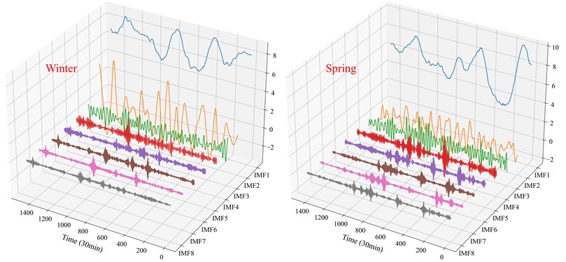
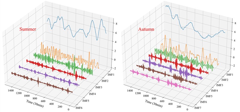
Table 5IMF center frequencies across different K settings (Winter)
K | IMF1 | IMF2 | IMF3 | IMF4 | IMF5 | IMF6 | IMF7 | IMF8 | IMF9 |
2 | 0.323x10⁻³ | 0.255 | – | – | – | – | – | – | – |
3 | 0.313x10⁻³ | 0.009 | 0.333 | – | – | – | – | – | – |
4 | 0.275x10⁻³ | 0.009 | 0.254 | 0.373 | – | – | – | – | – |
5 | 0.232x10⁻³ | 0.008 | 0.038 | 0.254 | 0.374 | – | – | – | – |
6 | 0.212x10⁻³ | 0.008 | 0.038 | 0.249 | 0.322 | 0.378 | – | – | – |
7 | 0.167x10⁻³ | 0.008 | 0.033 | 0.084 | 0.255 | 0.372 | 0.461 | – | – |
8 | 0.114x10⁻³ | 0.008 | 0.033 | 0.084 | 0.250 | 0.322 | 0.377 | 0.463 | – |
9 | 0.078x10⁻³ | 0.008 | 0.032 | 0.082 | 0.152 | 0.254 | 0.324 | 0.377 | 0.463 |
4.4. Wind speed reconstruction via fuzzy entropy
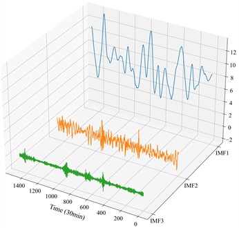
After VMD decomposition, the offshore wind speed time series is represented as a set of IMF components. Directly predicting all components may lead to increased computational complexity and error accumulation. To address this, the Fuzzy Entropy (FE) of each component is calculated to quantify its complexity. Components with similar FE values are grouped and reconstructed, reducing redundancy while preserving key dynamic patterns.
Based on the FE evaluation, IMFs with similar entropy levels were grouped to form low-, mid- and high-complexity components. Lower-entropy IMFs typically exhibited more regular oscillations, whereas higher-entropy IMFs contained richer dynamical variations and contributed more predictive information. This FE-guided reconstruction ensures that the retained components reflect distinct temporal behaviors while suppressing noise-dominated signals.
Fig. 10Fuzzy entropy analysis results for seasonal datasets
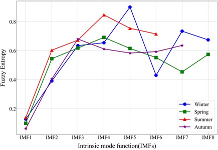
The FE values and seasonal differences are visualized in Fig. 10, which shows that complexity varies by season and IMF component. Taking the winter dataset as an example, this reconstruction result illustrated in Fig. 11, enables the generation of three clear sub-sequences with distinguishable frequency characteristics. Compared with the original full IMF set, the reconstructed sequences offer lower dimensionality and improved interpretability, which contributes to more robust and accurate prediction. It should be noted that the fuzzy entropy (FE) values of the IMFs differ across the four seasonal datasets. This variation arises because wind-speed time series exhibit distinct turbulence intensities and fluctuation characteristics under different seasonal meteorological conditions. Since FE measures the irregularity and complexity of a signal, the resulting entropy values naturally reflect these seasonal dynamics rather than remaining uniform across all datasets.
4.5. Comparison of forecasting techniques
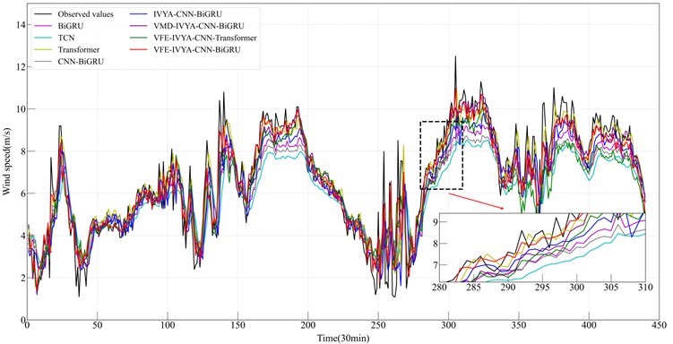
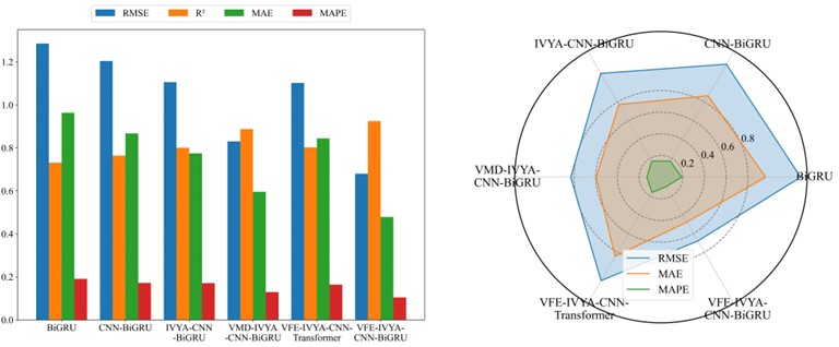
To thoroughly evaluate the proposed VFE-IVYA-CNN-BiGRU model, this study conducts a comparative assessment against five benchmark forecasting models: BiGRU, TCN, Transformer, CNN-BiGRU, IVYA-CNN-BiGRU, VMD-IVYA-CNN-BiGRU and VFE-IVYA-CNN-Transformer. The models are tested on four seasonal offshore wind speed datasets – winter, spring, summer, and autumn – and evaluated using MAE, RMSE, MAPE, and the coefficient of determination . Quantitative results are reported in Table 6 and visualized in Figs. 12–19.
Fig. 11Reconstructed wind speed signal after FE-based IMF filtering (Winter)
Among the four seasonal datasets, the winter results most clearly demonstrate the performance advantages of the proposed VFE-IVYA-CNN-BiGRU model. Winter wind speed series exhibit strong periodicity coupled with moderate low-frequency fluctuations, making this season an essential benchmark for evaluating multi-scale feature extraction and temporal-dependency modeling. On this dataset, the proposed model achieves an exceeding 0.97, significantly outperforming BiGRU (≈ 0.8860), TCN (≈ 0.8803), Transformer (≈ 0.8753), and CNN-BiGRU (≈ 0.9037), corresponding to a relative improvement of approximately 8.9-11.3 %. The reduction in error metrics is even more pronounced: compared with the basic BiGRU, the proposed architecture reduces MAE by more than 55 % and RMSE by nearly 60 %, indicating substantially enhanced accuracy in capturing both the amplitude variation and temporal evolution of winter wind speed. Even against stronger convolution-based baselines such as CNN-BiGRU and IVYA-CNN-BiGRU, MAE and RMSE still decrease by 40-50 % and 45-55%, respectively, demonstrating the synergistic benefits introduced by VFE decomposition and IVYA-enhanced convolution for representing localized structures and high-frequency fluctuations. Furthermore, relative to more advanced hybrid approaches – such as VMD-IVYA-CNN-BiGRU and VFE-IVYA-CNN-Transformer – the proposed model maintains clear superiority, achieving 15-25 % reductions in RMSE and 20-35 % reductions in MAPE. These improvements further highlight the decisive role of the BiGRU component in modeling long-range dependencies within winter’s quasi-stationary wind patterns.
The winter ablation results show a clear stepwise improvement as each module is added. Starting from the BiGRU baseline ( 0.8860), introducing CNN reduces MAE and RMSE by roughly 20-30 %, while replacing CNN with IVYA brings a further 10-15 % reduction. Adding VMD provides another 15–20% improvement in RMSE through more effective mode separation. With VFE incorporated, the model reaches 0.97 and achieves over 55 % and 60 % decreases in MAE and RMSE compared with BiGRU, confirming that each component contributes incremental and complementary gains.
By contrast, the spring, summer, and autumn datasets exhibit stronger irregularity and transitional seasonal characteristics, resulting in relatively narrower performance gaps among models. Nevertheless, the proposed method remains the top performer across all evaluation metrics, typically reducing RMSE by 10-20 % and MAPE by 10-25 % compared with the next-best model. In particular, for the highly non-stationary and fluctuation-intensive summer dataset, the proposed model improves by more than 30 % relative to BiGRU, confirming its strong adaptability under chaotic wind conditions. Overall, the winter experiments provide the clearest quantitative evidence of the method’ s core advantages: VFE ensures high-fidelity mode separation and mitigates modal mixing; IVYA-CNN enhances the extraction of local and high-frequency structures; and BiGRU delivers robust long-term dependency modeling. The synergistic integration of these components enables the proposed model to achieve the highest forecasting accuracy across all seasons, with winter exhibiting particularly substantial improvements.
Fig. 12Results from six forecasting approaches (Winter)
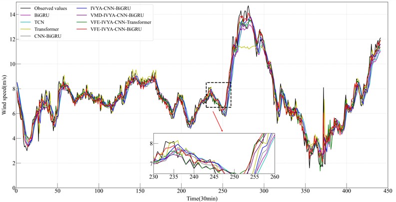
Fig. 13Results from six forecasting approaches (Spring)
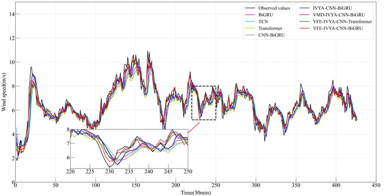
These statistical gains are corroborated by the time-series prediction plots (Figs. 12-15), where the proposed model demonstrates significantly better temporal alignment with ground truth, especially around peaks, troughs, and inflection zones. In winter and autumn, where daily amplitude varies widely, the model accurately follows trend direction without lag – whereas other models, especially BiGRU and CNN-BiGRU, show smoothing effects or phase shift. In summer, the proposed model shows reduced overfitting and higher responsiveness to random fluctuations, which is particularly evident in fast-changing segments.
Fig. 14Results from six forecasting approaches (Summer)
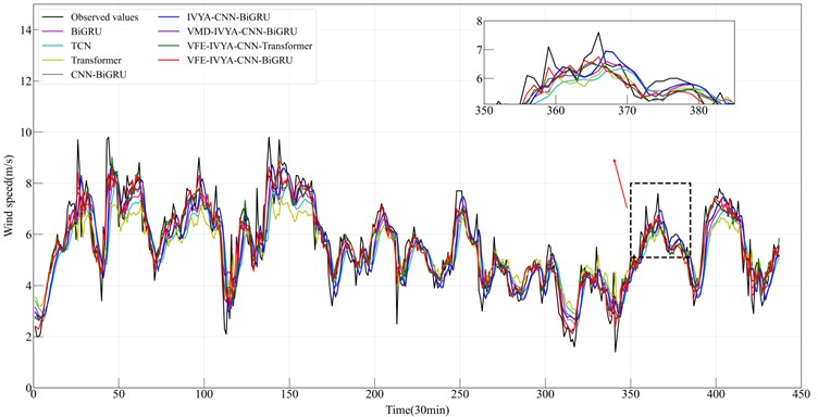
Fig. 15Results from six forecasting approaches (Autumn)
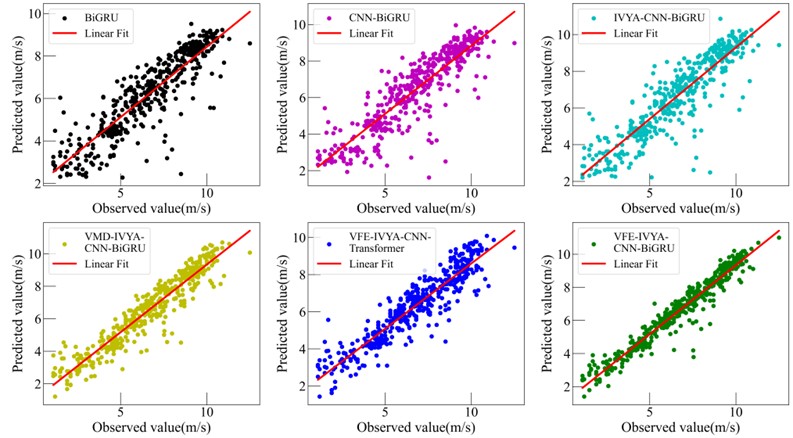
Visual evaluations from radar plots (Figs. 16-19) further emphasize the model's advantage. The VFE-IVYA-CNN-BiGRU consistently occupies the innermost region, indicating minimum error across all axes (MAE, RMSE, MAPE). In bar plots, the percentage decrease in MAE reaches up to 57.5 %, and MAPE up to 55.1 %, compared to the weakest models. Moreover, scatter-fitting plots reveal denser clustering near the identity line with a steeper slope closer to unity and reduced spread, reflecting both reduced bias and variance. The residual distribution is significantly narrower, especially in high-variance seasons, further confirming better model reliability.
The consistent improvement of the proposed model is attributed to the synergistic integration of three key components. The original signal is decomposed into a set of intrinsic mode functions (IMFs) using VMD, isolating multiscale oscillations and reducing non-stationarity. Fuzzy Entropy quantifies the complexity of each IMF, allowing the model to suppress low-informative or noise-prone components. This process produces a reconstructed sequence with a higher signal-to-noise ratio, which enhances learning stability. Finally, IVYA adaptively optimizes the model’s architecture – including convolutional depth, recurrent capacity, and learning parameters – resulting in efficient convergence and enhanced generalization across seasonal regimes.
In summary, the VFE-IVYA-CNN-BiGRU model exhibits not only lower average forecasting error but also superior temporal alignment, reduced sensitivity to extreme values, and better fit in noisy or high-variance conditions. Its performance advantage is both statistically significant and structurally grounded, enabling robust offshore wind speed forecasting across all seasonal contexts.
Fig. 16Comparative forecasting accuracy of six models (Winter)
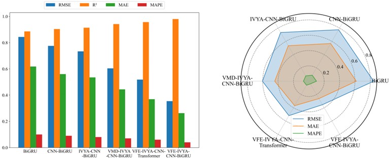
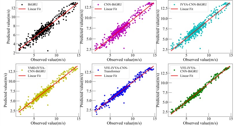
Fig. 17Comparative forecasting accuracy of six models (Spring)
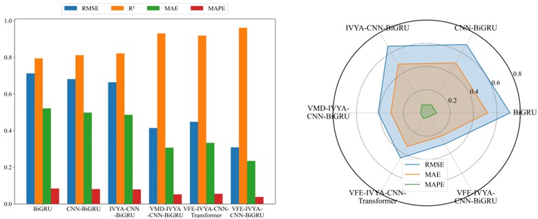
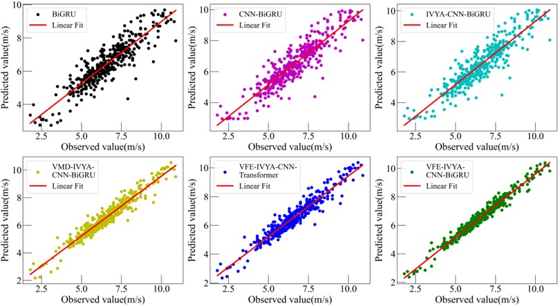
Fig. 18Comparative forecasting accuracy of six models (Summer)
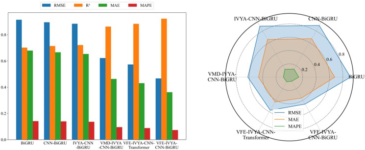
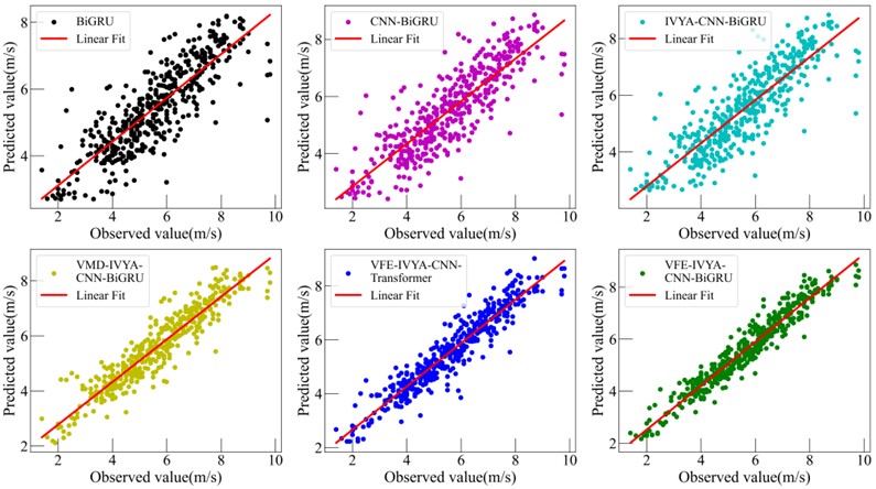
Fig. 19Comparative forecasting accuracy of six models (Autumn)
To further rule out the possibility of target leakage or artificially inflated performance caused by highly collinear meteorological variables, an additional ablation experiment was conducted on the winter dataset using the proposed VFE-IVYA-CNN-BiGRU model. In this test, the gust-speed variable (GSP), which exhibits the strongest correlation with wind speed, was removed from the input set. Excluding GSP led to a clear degradation in forecasting accuracy, with decreasing to 0.9322, MAE increasing to 0.4729 m/s, RMSE rising to 0.6536 m/s, and MAPE increasing to 7.864 %. This consistent deterioration confirms that the gust-related variable provides genuine predictive information rather than leaking future values or duplicating the target signal. The results further demonstrate that the proposed framework effectively captures physically meaningful meteorological drivers, and that the performance gains attributed to gust-related features arise from true model learning rather than from spurious correlations or unintended data leakage.
5. Model interpretability via SHAP
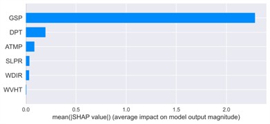
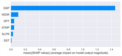
To enhance the interpretability and transparency of the VFE-IVYA-CNN-BiGRU model in offshore wind speed forecasting and assess the influence of each meteorological input variable on the model’s predictive behavior, SHAP (SHapley Additive exPlanations) was utilized. Visual analyses, including SHAP summary plots and mean absolute SHAP value bar charts, were produced for four representative months – January, April, July, and October – capturing seasonal variations across winter, spring, summer, and autumn, as illustrated in Figs. 20-21. These visualizations offer both global and instance-level insights into feature influence, facilitating a better understanding of model decision pathways under varying atmospheric conditions.
Table 6Forecasting performance comparison of all models in four seasons
Models | MAE (m/s) | RMSE (m/s) | MAPE | ||
Winter | BiGRU | 0.8860 | 0.6179 | 0.8438 | 10.1441 |
TCN | 0.8803 | 0.6408 | 0.8647 | 10.4430 | |
Transformer | 0.8735 | 0.5973 | 0.8887 | 9.8472 | |
CNN-BiGRU | 0.9037 | 0.5679 | 0.7753 | 9.2069 | |
IVYA-CNN-BiGRU | 0.9138 | 0.5350 | 0.7336 | 8.9219 | |
VMD-IVYA-CNN-BiGRU | 0.9416 | 0.4439 | 0.6040 | 7.3820 | |
VFE-IVYA-CNN-Transformer | 0.9569 | 0.3690 | 0.5185 | 6.3588 | |
VFE-IVYA-CNN-BiGRU | 0.9799 | 0.2625 | 0.3540 | 4.5538 | |
Spring | BiGRU | 0.7942 | 0.5215 | 0.7125 | 8.4240 |
TCN | 0.7242 | 0.6002 | 0.8248 | 9.7519 | |
Transformer | 0.7562 | 0.5876 | 0.7755 | 9.0019 | |
CNN-BiGRU | 0.8120 | 0.4983 | 0.6810 | 8.1204 | |
IVYA-CNN-BiGRU | 0.8213 | 0.4861 | 0.6639 | 7.9653 | |
VMD-IVYA-CNN-BiGRU | 0.9304 | 0.3068 | 0.4143 | 5.2021 | |
VFE-IVYA-CNN-Transformer | 0.9186 | 0.3333 | 0.4480 | 5.5608 | |
VFE-IVYA-CNN-BiGRU | 0.9613 | 0.2346 | 0.3091 | 3.8962 | |
Summer | BiGRU | 0.7015 | 0.6791 | 0.9141 | 14.1265 |
TCN | 0.6237 | 0.7810 | 1.0262 | 16.0545 | |
Transformer | 0.6706 | 0.7352 | 0.9602 | 15.1340 | |
CNN-BiGRU | 0.7138 | 0.6660 | 0.8949 | 13.9299 | |
IVYA-CNN-BiGRU | 0.7211 | 0.6534 | 0.8835 | 13.6726 | |
VMD-IVYA-CNN-BiGRU | 0.8618 | 0.4628 | 0.6220 | 9.5977 | |
VFE-IVYA-CNN-Transformer | 0.8827 | 0.4304 | 0.5729 | 8.8016 | |
VFE-IVYA-CNN-BiGRU | 0.9221 | 0.3616 | 0.4668 | 7.3373 | |
Autumn | BiGRU | 0.7312 | 0.9635 | 1.2855 | 19.1504 |
TCN | 0.6061 | 1.2333 | 1.5560 | 23.2109 | |
Transformer | 0.7008 | 1.0431 | 1.3561 | 20.8920 | |
CNN-BiGRU | 0.7640 | 0.8678 | 1.2045 | 17.2027 | |
IVYA-CNN-BiGRU | 0.8009 | 0.7746 | 1.1061 | 17.1277 | |
VMD-IVYA-CNN-BiGRU | 0.8879 | 0.5961 | 0.8302 | 12.9817 | |
VFE-IVYA-CNN-Transformer | 0.8023 | 0.8444 | 1.1024 | 16.4985 | |
VFE-IVYA-CNN-BiGRU | 0.9248 | 0.4788 | 0.6799 | 10.4956 |
In this study, we adopt the DeepSHAP variant of the SHAP framework, which is suitable for deep neural network architectures. To avoid data leakage, the SHAP background dataset is constructed exclusively from the training subset, using 200 randomly sampled instances to approximate the expected background distribution. SHAP values are computed on 100 representative samples from the test set to balance interpretability and computational efficiency. All SHAP computations are performed using the official SHAP Python package on a workstation equipped with an NVIDIA RTX 3080 GPU and Intel i9 processor. The SHAP analysis is performed on the sliding-window input representation of each sub-model. Each meteorological variable appears as multiple lagged instances within the window (e.g., gust(t−1), gust(t−2), …). SHAP assigns an attribution value to every lagged instance. To obtain a unified and physically meaningful importance measure for each meteorological variable, we aggregate the per-lag attributions by computing the mean absolute SHAP value across all time steps. Therefore, the reported SHAP results correspond to feature-level contributions, reflecting how each meteorological variable influences the final wind-speed prediction after passing through the full VFE-IVYA-CNN-BiGRU modeling pipeline.
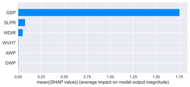
Fig. 20Mean absolute SHAP values for feature importance
a) Winter
b) Spring
c) Summer
d) Autumn
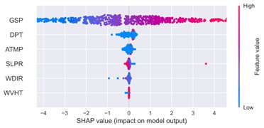
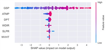
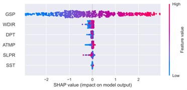
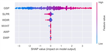
Fig. 21SHAP summary plot of feature impacts
a) Winter
b) Spring
c) Summer
d) Autumn
Across all seasonal datasets, gust speed (GSP) consistently ranked as the most influential feature, exhibiting the highest mean SHAP values. In the winter case, for example, GSP reached an average SHAP contribution exceeding 2.25, which is nearly an order of magnitude larger than those of dew point temperature (DPT, ~0.25) and air temperature (ATMP, ~0.12). The SHAP summary plot revealed a strongly monotonic positive relationship between GSP magnitude and its SHAP attribution: red markers, representing higher GSP values, are mostly concentrated on the right side of the SHAP distribution, suggesting a strong positive influence on predicted wind speed, whereas lower GSP values (in blue) generally lead to reduced predictions. This behavior is physically consistent with meteorological principles and persists across all seasonal contexts.
Thermal variables such as DPT and ATMP exhibited secondary but seasonally modulated effects. In spring, for instance, the SHAP values of both features increased, with high DPT and ATMP levels slightly elevating wind speed predictions. This suggests a potential interaction between thermodynamic factors and boundary-layer wind development during transitional periods. The color gradients in the SHAP plots – ranging from blue (low feature value) to red (high value) – further illustrate that mid-range DPT values tend to have minimal impact, while higher values contribute positively, albeit with increased sample-wise variance. This pattern indicates that the influence of temperature variables is likely non-linear and conditional on other atmospheric parameters such as sea-level pressure or humidity.
SLPR and WDIR, though showing relatively low average SHAP values, displayed episodic high contributions in specific cases – particularly in the autumn dataset. Their dispersed SHAP distributions, combined with red and blue color interleaving, imply non-monotonic and interaction-driven effects. For example, both high and low SLPR values can enhance or reduce wind speed predictions depending on the prevailing synoptic context. Notably, in some autumn samples, low SLPR values contributed negatively with SHAP values below –1.2, while high SLPR values slightly increased predictions, reflecting the known meteorological behavior where sharp pressure gradients (e.g., near frontal systems or cyclonic events) induce stronger winds.
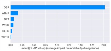
In the summer dataset, a general decline in SHAP intensity was observed for most features, indicating reduced feature influence under relatively stable atmospheric conditions. Nevertheless, GSP remained the dominant contributor, continuing to exhibit a positive and consistent relationship with the output. Interestingly, sea surface temperature (SST) emerged as a top-six feature during summer and autumn. Though its average SHAP values were modest (< 0.10), the presence of red-tinted SHAP points with slight positive impact suggests a possible secondary role in modulating wind dynamics, potentially linked to large-scale thermal forcing or ocean-atmosphere coupling.
The autumn dataset exhibited the broadest dispersion of SHAP values across features, implying a higher degree of variability in the contribution of secondary variables. GSP remained the dominant driver (mean SHAP ≈ 1.75), but SLPR and WDIR demonstrated greater sample-level variation than in other seasons. This variability aligns with the season’s complex synoptic patterns, including frontal passages and typhoon-related systems. For example, low SLPR values (blue) corresponded with reduced wind speed predictions, while high SLPR values (red) slightly elevated model outputs, in line with the physical mechanism of wind generation under steep pressure gradients.
In terms of global feature importance, bar charts consistently identified the same hierarchy across seasons: GSP ranked first, followed by thermal variables (DPT, ATMP), then pressure and direction (SLPR, WDIR). Wave-related variables (WVHT, AWP, DWP) displayed negligible average SHAP values (< 0.05), indicating minimal overall influence. However, the scattered distribution of their SHAP values in the summary plots suggests episodic relevance, likely under specific conditions such as storm surges or high swell events near the coast.
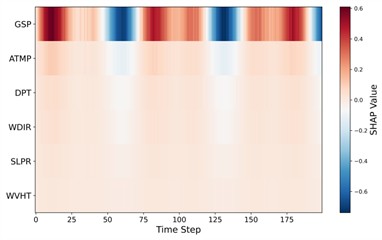
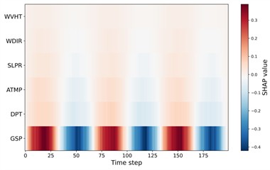
To further enhance interpretability and address the dynamic contribution of meteorological variables, this study incorporates time-resolved SHAP heatmaps for four representative seasonal datasets (winter, spring, summer, and autumn). Unlike aggregated SHAP importance scores, the time-resolved representation reveals how the influence of each input feature evolves across the sliding temporal window. Fig. 22 presents the seasonal SHAP heatmaps. A highly consistent pattern is observed across all seasons: GSP (gust speed) exhibits the strongest contribution with clear oscillatory structures over time, indicating its dominant role in driving short-term variability in offshore wind dynamics. This is meteorologically reasonable, as gust activity directly affects turbulence intensity and short-horizon wind speed fluctuations. Secondary features, such as ATMP, DPT, and SLPR, show weaker but smoother temporal contributions. These variables are mainly associated with synoptic-scale or mesoscale processes (e.g., temperature gradients, pressure fields), thus introducing more gradual variability in the prediction. Lower-ranked variables (e.g., WDIR, WVHT, SST, AWP, DWP) contribute only marginally and display minimal temporal fluctuations, consistent with their weaker physical relation to instantaneous wind speed.
Overall, the SHAP analysis confirms that the VFE-IVYA-CNN-BiGRU model aligns well with established meteorological understanding. Its predictions rely predominantly on physically interpretable variables such as gust speed, air temperature, and pressure, while also capturing non-linear and interaction effects that emerge under complex atmospheric conditions. The model's capacity to prioritize meaningful signals and modulate lesser features conditionally contributes to its superior performance. Importantly, such transparent behavior reinforces confidence in the model’s reliability and facilitates its deployment in real-world offshore wind forecasting systems, particularly in safety-critical or operation-sensitive applications. In this framework, SHAP values are computed directly on the original meteorological inputs, ensuring that the resulting attributions preserve their physical interpretability. Since each sub-model receives both the meteorological variables and the corresponding historical subcomponent as inputs, the SHAP results naturally reflect how meteorological drivers (e.g., gust, pressure, humidity) influence wind variations at different temporal scales. Consequently, the interpretability is not compromised by the preprocessing stage but rather enhanced, as the decomposition explicitly separates the physical scales of interest.
Fig. 22Time-resolved SHAP heatmap for feature contributions
a) Winter
b) Spring
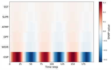
c) Summer
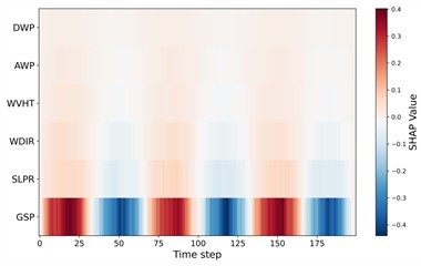
d) Autumn
6. Conclusions
To tackle the issues of nonlinear patterns, temporal instability, and insufficient interpretability in offshore wind speed forecasting, a new hybrid deep learning architecture, VFE-IVYA-CNN-BiGRU, was developed in this work. The model begins with feature selection using Pearson Correlation (PCs), which identifies the most relevant predictors from a set of nine meteorological variables. Subsequently, a robust preprocessing module (VFE), is designed to denoise the raw signal and reconstruct informative subcomponents. A CNN-BiGRU network is then employed to jointly extract temporal features, while the Ivy Algorithm (IVYA) adaptively optimizes key hyperparameters, leading to improved convergence and generalization across varying meteorological regimes.
Comprehensive experiments were conducted on real-world offshore wind datasets covering four representative seasons. The proposed model consistently outperformed five baseline methods across all evaluation metrics. Compared with the baseline BiGRU, the VFE-IVYA-CNN-BiGRU achieved average reductions in MAE and RMSE exceeding 50 %, and maintained values above 0.96 for all seasons. Visual analyses of prediction curves and residual distributions further confirmed the model’s ability to capture sharp transitions and irregular wind dynamics with high precision.
To enhance interpretability and increase model reliability, SHAP analysis was applied to reveal the internal decision-making process of the model. Results show that GSP was the most influential feature across all seasonal datasets, followed by temperature-related and pressure-related variables, depending on the seasonal context. The SHAP summary plots revealed that the model captures not only dominant monotonic trends but also non-linear and interaction-driven relationships, thereby aligning with physical meteorological principles and enhancing interpretability for real-world applications.
Despite the encouraging results, certain limitations remain. The current framework does not explicitly model temporal dependencies across turbines or stations, which may be crucial for large-scale wind farm forecasting. Moreover, the interpretability analysis is currently focused on global and marginal effects, with limited exploration of temporal or localized feature contributions. Future research will therefore aim to extend the model to spatiotemporal forecasting, implement real-time adaptive learning for abrupt weather transitions, and integrate probabilistic forecasting with uncertainty quantification to support decision-making under uncertainty.
In conclusion, the VFE-IVYA-CNN-BiGRU model offers a structurally integrated, interpretable, and highly accurate forecasting solution for short-term offshore wind speed prediction. Its performance, grounded in both data-driven learning and physically meaningful feature attribution, demonstrates significant potential for deployment in intelligent and reliable wind energy management system.
References
-
X. Xu, S. Hu, H. Shao, P. Shi, R. Li, and D. Li, “A spatio-temporal forecasting model using optimally weighted graph convolutional network and gated recurrent unit for wind speed of different sites distributed in an offshore wind farm,” Energy, Vol. 284, p. 128565, Dec. 2023, https://doi.org/10.1016/j.energy.2023.128565
-
J. Liu et al., “Life cycle cost modelling and economic analysis of wind power: A state of art review,” Energy Conversion and Management, Vol. 277, p. 116628, Feb. 2023, https://doi.org/10.1016/j.enconman.2022.116628
-
Z. Liu et al., “Challenges and opportunities for carbon neutrality in China,” Nature Reviews Earth and Environment, Vol. 3, No. 2, pp. 141–155, Dec. 2021, https://doi.org/10.1038/s43017-021-00244-x
-
Z. Gong, A. Wan, Y. Ji, K. Al-Bukhaiti, and Z. Yao, “Improving short-term offshore wind speed forecast accuracy using a VMD-PE-FCGRU hybrid model,” Energy, Vol. 295, p. 131016, May 2024, https://doi.org/10.1016/j.energy.2024.131016
-
H. Lu et al., “Wind direction prediction combined with wind speed in a wind farm,” Energy, Vol. 333, p. 137334, Oct. 2025, https://doi.org/10.1016/j.energy.2025.137334
-
J. Wang, Y. Liu, S. Shu, and X. He, “A coupling deterministic and probabilistic wind energy prediction based on information leakage prevention and distinctive deep learning network,” Engineering Applications of Artificial Intelligence, Vol. 152, p. 110862, Jul. 2025, https://doi.org/10.1016/j.engappai.2025.110862
-
M. Yang, R. Che, X. Yu, and X. Su, “Dual NWP wind speed correction based on trend fusion and fluctuation clustering and its application in short-term wind power prediction,” Energy, Vol. 302, p. 131802, Sep. 2024, https://doi.org/10.1016/j.energy.2024.131802
-
C. Ge et al., “Middle-term wind power forecasting method based on long-span NWP and microscale terrain fusion correction,” Renewable Energy, Vol. 240, p. 122123, Feb. 2025, https://doi.org/10.1016/j.renene.2024.122123
-
S. Khan, Y. Muhammad, I. Jadoon, S. E. Awan, and M. A. Z. Raja, “Leveraging LSTM-SMI and ARIMA architecture for robust wind power plant forecasting,” Applied Soft Computing, Vol. 170, p. 112765, Feb. 2025, https://doi.org/10.1016/j.asoc.2025.112765
-
G. V., K. Deepa, S. V. T. Sangeetha, P. T., J. Ramprabhakar, and N. Gowtham, “Uncertainty analysis of different forecast models for wind speed forecasting,” Renewable Energy, Vol. 241, p. 122285, Mar. 2025, https://doi.org/10.1016/j.renene.2024.122285
-
A.-H. Abdel-Aty, K. S. Nisar, W. R. Alharbi, S. Owyed, and M. H. Alsharif, “Boosting wind turbine performance with advanced smart power prediction: Employing a hybrid ARMA-LSTM technique,” Alexandria Engineering Journal, Vol. 96, pp. 58–71, Jun. 2024, https://doi.org/10.1016/j.aej.2024.03.078
-
Y. Altork, “Comparative analysis of machine learning models for wind speed forecasting: Support vector machines, fine tree, and linear regression approaches,” International Journal of Thermofluids, Vol. 27, p. 101217, May 2025, https://doi.org/10.1016/j.ijft.2025.101217
-
J. Wang, X. Niu, L. Zhang, Z. Liu, and X. Huang, “A wind speed forecasting system for the construction of a smart grid with two-stage data processing based on improved ELM and deep learning strategies,” Expert Systems with Applications, Vol. 241, p. 122487, May 2024, https://doi.org/10.1016/j.eswa.2023.122487
-
T. C. Akinci, H. Selcuk Nogay, M. Penchev, A. A. Martinez-Morales, and A. Raju, “A hybrid approach to wind power intensity classification using decision trees and large language models,” Renewable Energy, Vol. 250, p. 123388, Sep. 2025, https://doi.org/10.1016/j.renene.2025.123388
-
Y. Wang, X. Zhao, Z. Li, W. Zhu, and R. Gui, “A novel hybrid model for multi-step-ahead forecasting of wind speed based on univariate data feature enhancement,” Energy, Vol. 312, p. 133515, Dec. 2024, https://doi.org/10.1016/j.energy.2024.133515
-
K. F. Sotiropoulou, A. P. Vavatsikos, and P. N. Botsaris, “A hybrid AHP-PROMETHEE II onshore wind farms multicriteria suitability analysis using kNN and SVM regression models in northeastern Greece,” Renewable Energy, Vol. 221, p. 119795, Feb. 2024, https://doi.org/10.1016/j.renene.2023.119795
-
S. Ali, M. Waleed, and D. Lee, “A novel AI-based CNN model to predict the structural performance of monopile used for offshore wind energy systems,” Energy Conversion and Management: X, Vol. 26, p. 101028, Apr. 2025, https://doi.org/10.1016/j.ecmx.2025.101028
-
Q. Li, G. Wang, X. Wu, Z. Gao, and B. Dan, “Arctic short-term wind speed forecasting based on CNN-LSTM model with CEEMDAN,” Energy, Vol. 299, p. 131448, Jul. 2024, https://doi.org/10.1016/j.energy.2024.131448
-
H. Wang, Q. Ran, G. Ma, J. Wen, J. Zhang, and S. Zhou, “Optimization design of floating offshore wind turbine mooring system based on DNN and NSGA-III,” Ocean Engineering, Vol. 316, p. 119915, Jan. 2025, https://doi.org/10.1016/j.oceaneng.2024.119915
-
D. Yang, M. Li, J.-E. Guo, and P. Du, “An attention-based multi-input LSTM with sliding window-based two-stage decomposition for wind speed forecasting,” Applied Energy, Vol. 375, p. 124057, Dec. 2024, https://doi.org/10.1016/j.apenergy.2024.124057
-
A. Wan et al., “A novel hybrid BWO-BiLSTM-ATT framework for accurate offshore wind power prediction,” Ocean Engineering, Vol. 312, p. 119227, Nov. 2024, https://doi.org/10.1016/j.oceaneng.2024.119227
-
M. Hu, G. Zheng, Z. Su, L. Kong, and G. Wang, “Short-term wind power prediction based on improved variational modal decomposition, least absolute shrinkage and selection operator, and BiGRU networks,” Energy, Vol. 303, p. 131951, Sep. 2024, https://doi.org/10.1016/j.energy.2024.131951
-
D. Geng, Y. Zhang, Y. Zhang, X. Qu, and L. Li, “A hybrid model based on CapSA-VMD-ResNet-GRU-attention mechanism for ultra-short-term and short-term wind speed prediction,” Renewable Energy, Vol. 240, p. 122191, Feb. 2025, https://doi.org/10.1016/j.renene.2024.122191
-
V. Namboodiri V. and R. Goyal, “A novel hybrid ensemble wind speed forecasting model employing wavelet transform and deep learning,” Computers and Electrical Engineering, Vol. 121, p. 109820, Jan. 2025, https://doi.org/10.1016/j.compeleceng.2024.109820
-
Z. Xiong, J. Yao, Y. Huang, Z. Yu, and Y. Liu, “A wind speed forecasting method based on EMD-MGM with switching QR loss function and novel subsequence superposition,” Applied Energy, Vol. 353, p. 122248, Jan. 2024, https://doi.org/10.1016/j.apenergy.2023.122248
-
B. Wu and L. Wang, “Two-stage decomposition and temporal fusion transformers for interpretable wind speed forecasting,” Energy, Vol. 288, p. 129728, Feb. 2024, https://doi.org/10.1016/j.energy.2023.129728
-
W. Liu, Y. Bai, X. Yue, R. Wang, and Q. Song, “A wind speed forecasting model based on rime optimization based VMD and multi-headed self-attention-LSTM,” Energy, Vol. 294, p. 130726, May 2024, https://doi.org/10.1016/j.energy.2024.130726
-
Y. Liang, D. Zhang, J. Zhang, and G. Hu, “A state-of-the-art analysis on decomposition method for short-term wind speed forecasting using LSTM and a novel hybrid deep learning model,” Energy, Vol. 313, p. 133826, Dec. 2024, https://doi.org/10.1016/j.energy.2024.133826
-
C. Wang, H. Lin, H. Hu, M. Yang, and L. Ma, “A hybrid model with combined feature selection based on optimized VMD and improved multi-objective coati optimization algorithm for short-term wind power prediction,” Energy, Vol. 293, p. 130684, Apr. 2024, https://doi.org/10.1016/j.energy.2024.130684
-
F. Di Maio, C. Pettorossi, and E. Zio, “Entropy-driven Monte Carlo simulation method for approximating the survival signature of complex infrastructures,” Reliability Engineering and System Safety, Vol. 231, p. 108982, Mar. 2023, https://doi.org/10.1016/j.ress.2022.108982
-
J. Zhu, W. Bai, J. Zhao, L. Zuo, T. Zhou, and K. Li, “Variational mode decomposition and sample entropy optimization based transformer framework for cloud resource load prediction,” Knowledge-Based Systems, Vol. 280, p. 111042, Nov. 2023, https://doi.org/10.1016/j.knosys.2023.111042
-
Y. Liu et al., “CEEMDAN fuzzy entropy based fatigue driving detection using single-channel EEG,” Biomedical Signal Processing and Control, Vol. 95, p. 106460, Sep. 2024, https://doi.org/10.1016/j.bspc.2024.106460
-
G. Xin and L. Ying, “Multi-attribute decision-making based on comprehensive hesitant fuzzy entropy,” Expert Systems with Applications, Vol. 237, p. 121459, Mar. 2024, https://doi.org/10.1016/j.eswa.2023.121459
-
Z. Liu and H. Liu, “A novel hybrid model based on GA-VMD, sample entropy reconstruction and BiLSTM for wind speed prediction,” Measurement, Vol. 222, p. 113643, Nov. 2023, https://doi.org/10.1016/j.measurement.2023.113643
-
X. Sun and H. Liu, “Multivariate short-term wind speed prediction based on PSO-VMD-SE-ICEEMDAN two-stage decomposition and Att-S2S,” Energy, Vol. 305, p. 132228, Oct. 2024, https://doi.org/10.1016/j.energy.2024.132228
-
H. Sun, Q. Cui, J. Wen, L. Kou, and W. Ke, “Short-term wind power prediction method based on CEEMDAN-GWO-Bi-LSTM,” Energy Reports, Vol. 11, pp. 1487–1502, Jun. 2024, https://doi.org/10.1016/j.egyr.2024.01.021
-
C. Zhang, W. Lin, and G. Hu, “An enhanced ivy algorithm fusing multiple strategies for global optimization problems,” Advances in Engineering Software, Vol. 203, p. 103862, May 2025, https://doi.org/10.1016/j.advengsoft.2024.103862
-
W. Liao, J. Fang, L. Ye, B. Bak-Jensen, Z. Yang, and F. Porte-Agel, “Can we trust explainable artificial intelligence in wind power forecasting?,” Applied Energy, Vol. 376, p. 124273, Dec. 2024, https://doi.org/10.1016/j.apenergy.2024.124273
-
Y. Sun, Y. Li, R. Wang, and R. Ma, “Modelling potential land suitability of large-scale wind energy development using explainable machine learning techniques: Applications for China, USA and EU,” Energy Conversion and Management, Vol. 302, p. 118131, Feb. 2024, https://doi.org/10.1016/j.enconman.2024.118131
-
F. Ren and X. Cao, “Wind power prediction based on VMD-BWO-KELM,” Electric Power Systems Research, Vol. 247, p. 111765, Oct. 2025, https://doi.org/10.1016/j.epsr.2025.111765
-
D. Deng et al., “Feature selection based on fuzzy joint entropy and feature interaction for label distribution learning,” Information Processing and Management, Vol. 62, No. 6, p. 104234, Nov. 2025, https://doi.org/10.1016/j.ipm.2025.104234
-
M. Ghasemi, M. Zare, P. Trojovský, R. V. Rao, E. Trojovská, and V. Kandasamy, “Optimization based on the smart behavior of plants with its engineering applications: Ivy algorithm,” Knowledge-Based Systems, Vol. 295, p. 111850, Jul. 2024, https://doi.org/10.1016/j.knosys.2024.111850
-
R. Luo, Y. Li, H. Guo, Q. Wang, and X. Wang, “Cross-operating-condition fault diagnosis of a small module reactor based on CNN-LSTM transfer learning with limited data,” Energy, Vol. 313, p. 133901, Dec. 2024, https://doi.org/10.1016/j.energy.2024.133901
-
Y. Bai et al., “Research on steel structure damage detection based on TCD-CNN method,” Structures, Vol. 57, p. 105318, Nov. 2023, https://doi.org/10.1016/j.istruc.2023.105318
-
K. Zhang et al., “SOH estimation of battery based on the BIGRU-transformer algorithm considering the hierarchical voltage interval characterization of the discharge curve,” Journal of Energy Storage, Vol. 132, p. 117770, Oct. 2025, https://doi.org/10.1016/j.est.2025.117770
-
L. Fu, T. Wang, M. Ouyang, L. Zhao, and X. Yin, “ATCN-BiGRU: A hybrid deep learning framework based temporal convolutional network and stacked bidirectional gate recurrent units for traffic flow prediction in urban scenarios,” Engineering Applications of Artificial Intelligence, Vol. 158, p. 111473, Oct. 2025, https://doi.org/10.1016/j.engappai.2025.111473
-
S. Ruan et al., “Multifactor interpretability method for offshore wind power output prediction based on TPE-CatBoost-SHAP,” Computers and Electrical Engineering, Vol. 123, p. 110081, Apr. 2025, https://doi.org/10.1016/j.compeleceng.2025.110081
-
C. Cakiroglu, S. Demir, M. Hakan Ozdemir, B. Latif Aylak, G. Sariisik, and L. Abualigah, “Data-driven interpretable ensemble learning methods for the prediction of wind turbine power incorporating SHAP analysis,” Expert Systems with Applications, Vol. 237, p. 121464, Mar. 2024, https://doi.org/10.1016/j.eswa.2023.121464
-
A. Ghaffar, W. Huo, Y. Qamar, H. Garg, and S. Ghafoor, “A novel combined framework for short-term wind speed forecasting based on data preprocessing with sequence reconstruction and Grey Wolf optimization,” Energy Reports, Vol. 14, pp. 1251–1272, Dec. 2025, https://doi.org/10.1016/j.egyr.2025.06.039
-
X. Chen, X. Ye, J. Shi, Y. Zhang, and X. Xiong, “A spatial transfer-based hybrid model for wind speed forecasting,” Energy, Vol. 313, p. 133920, Dec. 2024, https://doi.org/10.1016/j.energy.2024.133920
-
H. Elmousalami, H. H. Elmesalami, M. Maxi, A. A. K. M. Farid, and N. Elshaboury, “A comprehensive evaluation of machine learning and deep learning algorithms for wind speed and power prediction,” Decision Analytics Journal, Vol. 13, p. 100527, Dec. 2024, https://doi.org/10.1016/j.dajour.2024.100527
About this article

We are very grateful for the support of the project “Research on Multi-energy Complementary Integrated Scheduling and Control Technology” (Contract No. Z242302011) of China Yangtze River Power Co., Funding for Jiangsu Province University Science and Technology Innovation Team Project, and 2024 Annual Jiangsu Provincial Education Science Planning Project (Project No.: C/2024/02/48).
The datasets generated during and/or analyzed during the current study are available from the corresponding author on reasonable request.
Peifang Liu: writing-original draft, writing-review and editing, software, validation, visualization. Jiang Guo: conceptualization, funding acquisition, supervision. Ye Zou: conceptualization, funding acquisition, data curation. Nana Gao: methodology, formal analysis, funding acquisition.
The authors declare that they have no conflict of interest.
