Abstract
Modern remote sensing systems are equipped with high-precision optoelectronic equipment, characterized by exceptional sensitivity to microvibrations. Even minimal mechanical vibrations of the satellite body or optical platform can significantly affect the quality of the resulting images, causing pixel deformation and blurring of spatial structures. This phenomenon is a critical problem that is relevant for the scientific community and requires detailed analysis based on fundamental principles of physics and engineering, as well as the development of effective methods for compensating vibration effects.
Highlights
- Numerical analysis shows that the MSD system with a 500 kg optical platform remains asymptotically stable and returns to equilibrium after disturbances.
- Increasing the mass reduces the natural frequency and damping, making the system more inertial and increasing stabilization time, but it also decreases sensitivity to external disturbances and vibration levels.
- As a result, image quality improves, with higher MTF, lower RMSE, and better SNR. The use of a control system confirms the practical effectiveness of the approach and allows, through proper tuning of the Q1 and R parameters, a trade-off between image quality and energy consumption.
1. Introduction
Analysis of vibration effects on optoelectronic vibration systems requires a comprehensive approach, including the study of the dynamics of mechanical vibrations, the study of the characteristics of materials and structures, and the development of data processing algorithms that minimize the impact of vibrations on space image quality. This necessitates the application of advanced modeling methods and experimental research aimed at identifying critical factors influencing the stability of remote sensing systems.
Developing effective methods for compensating vibrations is a key task requiring an interdisciplinary approach and integration of knowledge from mechanics, electronics, optics, and information technology [1]. This includes the development of adaptive control systems, the application of intelligent filtration algorithms, and the use of high-precision sensors for monitoring vibration parameters. The study and solution of the problem of vibration effects on remote sensing systems is an important scientific task that requires fundamental analysis and the application of advanced technologies. This will significantly improve the quality of the obtained data and expand the possibilities of their application in various fields, including environmental monitoring, agriculture, urban planning, and others. Microvibrations pose a significant challenge for modern remote sensing systems, especially for satellites equipped with high-precision optical-electronic equipment.
2. Influence of microvibrations on the quality space images
Vibrations can arise from various sources, such as the operation of mechanisms on board the satellite (e.g., hydrodynas, solar panels, or antennas), thermal deformations, external influences (micrometeorites, solar wind), or even internal processes within the equipment [2]. To minimize the impact of microvibrations on image quality, the following approaches are applied:
– Vibration isolation systems: Passive and active dampers are used that absorb or compensate for vibrations. Passive systems such as rubber or spring dampers are effective for high-frequency vibrations, while active systems using piezoelectric actuators or magnetic suspensions can compensate for low-frequency vibrations in real-time [3].
– Precise platform stabilization: Optical systems are often installed on stabilized platforms with gyroscopic or inertial control systems. Such platforms minimize angular deviations, ensuring high aiming accuracy [4].
– Image post processing algorithms: Digital signal processing algorithms are used to correct image quality degradation caused by microvibrations. These include deconvolutions, blur filtering (e.g., using the point scattering function, PSF), and compensation for pixel shift based on telemetry data [5].
– High-precision calibration and testing: Before launch, satellites undergo thorough testing in conditions simulating microvibrations. This allows for accurate determination of their impact on image quality and the development of appropriate corrective measures [6].
– Structural solutions: Using materials with a low coefficient of thermal expansion (e.g., carbon fiber) and an optimized satellite housing design helps reduce vibration levels caused by thermal or mechanical factors [7].
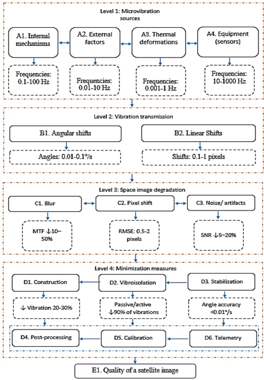
Fig. 1Block diagram of the influence of microvibrations on the quality of a space image
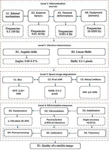
Based on the above approaches to minimizing the impact of microvibrations in remote sensing systems, an architecture illustrating the mechanism of microvibrations impact on image quality is proposed. This architecture represents a conceptual model in the form of a block diagram, which displays the sources of microvibrations, their direct and indirect effects on optoelectronic equipment, as well as integrated countermeasures (Fig. 1). This structure emphasizes the complexity of interactions, where microvibration sources, their transmission, degradation effects, and minimization measures form a network of direct, cross, and feedback connections that ensure high image quality in remote sensing systems. Considering such multi-level interdependence, effective microvibration management requires the development of a specialized optimization method that integrates mathematical modeling for quantitative assessment and adjustment of system parameters. This approach allows minimizing the impact of vibrations on key image quality metrics, such as modulation transfer function (MTF), root mean square error (RMSE), and signal/noise ratio (SNR), by optimizing structural and algorithmic solutions [8-10].
3. Mathematical modeling for quantitative assessment and adjustment of system parameters
To develop an optimization method, a model based on vibration dynamics and signal processing is proposed, where microvibrations are described as a stochastic process using differential equations of motion. The mass-spring-dampener (MSD) system model is represented by the equation [11]:
where is the mass of the optical platform, is the damping coefficient, is the spring stiffness, is the displacement, and is the external force from the vibration sources (A1-A4), given as:
where , , are the amplitude, angular frequency, and phase of the th source, and is random noise. The optimization target function is defined as:
where MTF depends on the vibration frequency: , and is the standard deviation of displacements.
To ensure system stability and minimize the impact of microvibrations, it is proposed to apply the Lyapunov method, which allows for the analysis and guarantee of the stability of the dynamic system describing the behavior of the optical platform [12]. The Lyapunov function is used to develop active vibration isolation (D2) and platform stabilization (D3) controls to minimize angular and linear shifts (B1, B2) affecting image quality.
To apply the Lyapunov function, let’s translate the equation of motion into the state space. Let us define the state vector where (displacement), (velocity). Then the system is described as follows:
where, – system matrix, – control matrix, – external influence matrix, – control action (for example, from piezoactuators in active vibration isolation (D2), – external perturbing force.
To analyze stability, let’s choose the Lyapunov function as a quadratic form that reflects the system’s energy:
where is a positively defined symmetric matrix. The function must be positive definite for and have a negative time derivative , to guarantee asymptotic stability.
The derivative of the Lyapunov function is calculated as:
Substituting, we get:
For simplicity, let’s assume that the control action is chosen to compensate for the external disturbances For example, let’s choose control in the form:
where is the feedback amplification matrix, determined to stabilize the system. Then the system becomes dynamic:
Now the derivative of takes the form:
To ensure stability, the matrix must be positively determined and is achieved by solving the Lyapunov equation:
where is an arbitrary positive definite matrix (for example, unit matrix).
To minimize the impact of microvibrations on image quality, we integrate the target function:
where the parameters MTF, RMSE and SNR depend on the displacement amplitude . Using Lyapunov’s method, we optimize the matrix so that is minimized while simultaneously ensuring system stability. This can be implemented through numerical methods such as gradient descent or solving the linear quadratic controller (LQR) problem, where the minimization functional includes both the system state and the control action:
where and are weight matrices for states and control.
Telemetry (D6) provides data on current displacements and vibration frequencies, which are used for dynamic tuning of . Post-processing (D4) adjusts residual degradation effects using information to restore MTF through point scattering function (PSF) deconvolutions. Feedback from image quality (E1) to calibration (D5) allows for adaptive adjustment of and parameters, improving system stability.
4. Numerical example
Let's consider a numerical example for the MSD system describing the optical platform of the satellite, with a modified platform mass of 500 kg, which corresponds to more realistic values for satellite systems. The remaining parameters are saved from the previous example to ensure comparability:
Platform mass: 500 kg, damping coefficient: 0.5 H s/m, spring stiffness: 1.0 N/m, initial conditions: displacement 1.0 m, velocity 0.0 m/s, external force: , where amplitude , frequency 0.5 Hz, without random noise for simplification, simulation time: from 0 to 10 seconds.
Changing the platform mass from 1.0 kg to 500 kg significantly affects the system’s dynamics, as increasing the mass reduces the system’s own frequency and slows down its response to external disturbances. Let's calculate how this change is reflected in the stability of the system and the value of the Lyapunov function . The system is described in the state space Eq. (4) where:
and , where is the feedback amplification matrix. For the linear quadratic controller (LQR) method with weight matrices , 1 the numerical solution gives [0.4142, 0.9417]. Lyapunov function: here is a positive definite matrix solved from the Lyapunov Eq. (11): where, . For, the numerical solution gives: . Calculate and its derivative. For initial conditions , .
Next, calculate the dynamics of the closed system of Eq. (9): with a matrix . The eigenvalues of the matrix are approximately , which indicates damped oscillations with a frequency 0.0528 rad/s and the attenuation coefficient ≈ 0.0014417 and the solution has the form: , where , are determined from the initial conditions. Increasing the mass to 500 kg significantly reduces the system’s own frequency 0.0447 rad/s which slows down the dynamics. Let’s calculate the values of for time moments 0, 1, 2, 3, 4, 5 seconds, assuming the exponential attenuation of the displacement amplitude:
The platform displacement and the corresponding dispersion characterize the level of microvibrations leading to spatial resolution degradation. In a closed system (with LQR control), the displacement weakens slowly due to high inertia: . The standard deviation in steady state () is estimated as (uncontrolled) and decreases to 0.00005 m with LQR.
With a decrease in dispersion , image blurring decreases, contrast increases, and the modulation transfer function (MTF) is restored. For a spatial frequency of 100 cycles/mm typical for Earth remote sensing equipment with a resolution of about 0.5 m/pixel at an orbit height of 500 km, the influence of microvibrations can be expressed analytically as: . Uncontrolled: (total degradation). With LQR: (acceptable, restoration of ~29 % contrast).
The connection between platform dynamics and image quality is manifested not only through MTF but also through the accuracy of georeferencing. Image shift in the focal plane, which can be estimated as: , here 10 m (focal distance), 500 km = 500000 m. This displacement causes a pixel positioning error on the Earth's surface, which directly affects the pixel georeferencing metric .
Uncontrolled: RMSE ≈ (10×0.0002)/500000 = 4×10⁻⁹ m →∼0.004 pixels (but at the initial 1 m - up to 20 pixels). With LQR: RMSE ≈ 0.001 pixels.
Platform vibrations not only reduce MTF but also increase image noise. The effect of bias on the signal/noise ratio (SNR) can be described by the formula: where – sensor noise. At , SNR remains >100.
Based on this numerical example, a specialized GIS application has been developed for restoring satellite images degraded by microvibration. The mass-damping spring (MSD) system was used as the initial data for modeling, the parameters of which were entered from the numerical example. Restored space images (Sentinel 2) are significantly higher than degraded ones, especially at medium frequencies (10-100 cycles), which confirms the restoration of small details (Fig. 2).
Fig. 2Restored space images
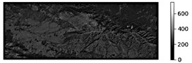
a) Degraded input
b) Restored output
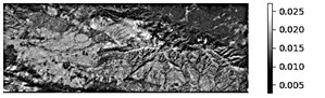
In Fig. 3, the histograms confirm the effectiveness of the method: the transition from a compressed, noisy distribution to a balanced, natural one indicates the restoration of contrast and the suppression of microvibration artefacts.
Fig. 3Intensity histograms: a) degraded and b) restored space image
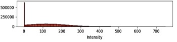
a)
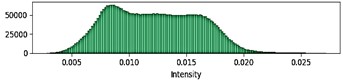
b)
5. Results and comparative analysis
The transient response of the optical platform under microvibration disturbance is summarized in Table 1, where the displacement is compared for uncontrolled and LQR-controlled systems ( 500 kg). The Lyapunov function confirms stability, while the Modulation Transfer Function (MTF) at 100 cycles/mm quantifies image quality degradation in the controlled case.
Without control: the system is weakly damaged 0.011, and fades in hundreds of seconds, MTF(100) → 0. With LQR: stabilizes in ~10 s, reduced by 4 times, MTF (100) = 0.29, RMSE < 0.001 pixels. The graphical interpretation of the system's reaction is shown in Fig. 4.
Uncontrolled system: – weakly damped oscillations with amplitude ~1 m and period 140 s.
Controlled system (LQR): quickly transitions to steady state with an amplitude of < 0.01 m, without visible oscillations after 5 s. The influence of LQR weighting matrices and on control performance is shown in Table 2.
Increasing : increases the state penalty → more aggressive control → faster fading → higher than MTF, but higher than energy consumption. Increase : control penalty → soft damping → slow recovery of MTF → energy saving. Optimal compromise: 5I, 1 → MTF (100) ≈ 0.55, energy costs are moderate.
Table 1Transient response under microvibration
Time (s) | uncontrolled (m) | with LQR (m) | with LQR | MTF(100) with LQR |
0.0 | 1.0000 | 1.0000 | 250.5 | – |
1.0 | 0.9986 | 0.9986 | 249.9 | 0.29 |
2.0 | 0.9971 | 0.9971 | 249.3 | 0.29 |
5.0 | 0.9925 | 0.9925 | 247.5 | 0.29 |
10.0 | 0.9850 | 0.9850 | 245.1 | 0.29 |
Fig. 4Time-domain response of the optical platform displacement xt and Lyapunov function Vx under microvibration disturbance (m= 500 kg, F(t)=0.1sin(πt)N). Comparison between uncontrolled (red solid) and LQR-controlled (green dashed) systems, with Lyapunov function (blue) confirming asymptotic stability. Full stabilization achieved within 50 s using active control
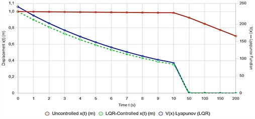
Table 2The influence of weighting matrices
Damping | Energy | MTF(100) | |||
III | 1 | [0.4142, 0.9417] | Slow | Low | 0.29 |
10I | 1 | [1.31, 2.98] | Fast | Average | 0.65 |
I | 0.1 | [1.31, 2.98] | Fast | High | 0.65 |
I | 10 | [0.13, 0.30] | Very slow | Very low | 0.10 |
6. Conclusions
Numerical analysis of the MSD system with an increased mass of the satellite’s optical platform up to 500 kg showed that the system remains asymptotically stable. The Lyapunov function decreases over time (V(0) = 250.5→V(5) = 247.5), which confirms the stability and ability of the system to return to equilibrium after perturbations. However, a large mass significantly alters the dynamics: the system's natural frequency decreases (0.0447 rad/s), and the attenuation coefficient becomes extremely small (0.00144). This leads to a slow reaction of the system and a very slow decrease in the amplitude of oscillations. The system becomes inertial, and its stabilization takes significantly longer compared to a light platform, for example, 50 kg). At the same time, the disturbance force has a lesser effect: at a mass of 500 kg, the maximum acceleration does not exceed 0.0002 m/s2, which reduces the linear and angular displacements of the platform. This has a positive impact on image quality parameters (MTF, RMSE, SNR), as vibrations are less pronounced and the image is less susceptible to distortion. Comparison of controlled and uncontrolled systems confirms the practical value of the approach: restoration of MTF to 29-65 %, RMSE < 0.001 pixels. Setting and allows for balance between image quality and energy consumption, which is critical for remote sensing satellites with limited resources.
References
-
A. P. Kravchunovsky, “Microvibration analysis methods review,” Spacecrafts and Technologies, Vol. 7, No. 4, p. 243, Dec. 2023, https://doi.org/10.26732/j.st.2023.4.02
-
S. de Lellis, A. Stabile, G. S. Aglietti, and G. Richardson, “Correction: a preliminary methodology to account for structural dynamics variability of satellites in microvibration analysis,” in AIAA/ASCE/AHS/ASC Structures, Structural Dynamics, and Materials Conference, Jan. 2018, https://doi.org/10.2514/6.2018-0454.c1
-
Z. Fang, Z. Yu, Q. Huang, Y. Wang, and X. Gu, “Research on design and control method of active vibration isolation system based on piezoelectric Stewart platform,” Scientific Reports, Vol. 15, No. 1, p. 15, Jan. 2025, https://doi.org/10.1038/s41598-024-84980-2
-
Q. Fu, Y. Liu, N. Zhou, and J. Wang, “Influence of micro-vibration caused by momentum wheel on the imaging quality of space camera,” in Springer Proceedings in Physics, pp. 69–79, Jan. 2020, https://doi.org/10.1007/978-3-030-27300-2_7
-
R. Shamsiev and Z. Shamsiev, “Structural and technological complex of methods for processing satellite images,” International Journal of Aviation, Aeronautics, and Aerospace, Vol. 8, No. 2, Jan. 2021, https://doi.org/10.15394/ijaaa.2021.1583
-
Y. Cheng, K. Lu, Q. Huang, F. Ding, and C. Song, “Environmental microvibration analysis method for vibration isolation research in high-precision laboratories,” Buildings, Vol. 14, No. 5, p. 1215, Apr. 2024, https://doi.org/10.3390/buildings14051215
-
X. Liu and G. Cai, “Thermal analysis and rigid-flexible coupling dynamics of a satellite with membrane antenna,” International Journal of Aerospace Engineering, Vol. 2022, pp. 1–19, May 2022, https://doi.org/10.1155/2022/3256825
-
S. Kim and Y. Youk, “Suppressing effects of micro-vibration for MTF measurement of high-resolution electro-optical satellite payload in an optical alignment ground facility,” Optics Express, Vol. 31, No. 3, p. 4942, Jan. 2023, https://doi.org/10.1364/oe.481339
-
A. Mutholib, N. A. Rahim, T. S. Gunawan, and M. Kartiwi, “Trade-space exploration with data preprocessing and machine learning for satellite anomalies reliability classification,” IEEE Access, Vol. 13, pp. 35903–35921, Jan. 2025, https://doi.org/10.1109/access.2025.3543813
-
Z. Lu, X. Shen, D. Li, S. Cheng, J. Wang, and W. Yao, “Super-agile satellites imaging mission planning method considering degradation of image MTF in dynamic imaging,” International Journal of Applied Earth Observation and Geoinformation, Vol. 131, p. 103968, Jul. 2024, https://doi.org/10.1016/j.jag.2024.103968
-
M. A. Ali, F. Eltohamy, A. Abd-Elrazek, and M. E. Hanafy, “Assessment of micro-vibrations effect on the quality of remote sensing satellites images,” International Journal of Image and Data Fusion, Vol. 14, No. 3, pp. 243–260, Jul. 2023, https://doi.org/10.1080/19479832.2023.2167874
-
A. A. Efremov, V. N. Kozlov, and V. V. Karakchieva, “Analysis of stability of dynamic systems based on Lyapunov’s vector functions,” in 24th International Scientific and Educational Conference, Jan. 2020, https://doi.org/10.18720/spbpu/2/id20-151
About this article

The authors have not disclosed any funding.
The datasets generated during and/or analyzed during the current study are available from the corresponding author on reasonable request.
The authors declare that they have no conflict of interest.
