Abstract
Considering that the dynamic analysis of mechanical systems with clearance needs to compile complex calculation programs, and high-precision numerical simulation is limited by computer performance. Dynamics of a two-degree-of-freedom system with soft impact are revealed from the perspective of equivalent circuit simulation in this paper. By using bifurcation diagrams and phase diagrams based on Poincaré mapping, as well as Lyapunov exponents, the mechanism of single-period multi-impact - motion and chattering impact under low-frequency conditions was revealed. In the MultiSim14.0 environment, a circuit diagram equivalent to the mathematical model of the system is designed by using the addition circuit, integration circuit, and inverter circuit composed of operational amplifiers, resistors, and capacitors. The nonlinear module is realized by the saturation characteristics of the operational amplifier. It is found that the output waveform of the virtual oscilloscope has a very good agreement with that obtained from the numerical simulation. Equivalent circuit test method not only has fast operation speed and less time consumption, but also can realize real-time dynamic adjustment of parameters, which provides a reference method for the dynamic research of mechanical system with clearance.
Highlights
- Essential features of one-period multi-impact 1-p-p motion and chattering-impact characteristics in low-frequency range are revealed from the perspective of equivalent circuit simulation.
- An electronic circuit schematic diagram equivalent to the mathematical model of the system is designed by using the addition circuit, integral circuit and inverse circuit composed of operational amplifier, resistor and capacitor.
- The nonlinear module is realized by the saturation characteristics of the operational amplifier.
- The dynamic characteristics of the system under different excitation frequencies and clearance thresholds can be obtained by changing the input frequency and voltage amplitude.
1. Introduction
The dynamic study of piecewise-smooth mechanical systems aims to elucidate the complex behaviors induced by non-smooth factors such as clearance, constraints, and friction, and related research has attracted significant attention [1-6]. For mechanical systems, due to factors such as lubricant film or thermal expansion and contraction, clearance must be intentionally provided in the design of certain equipment. Some equipment may experience clearance due to wear and tear caused by service or errors during manufacturing and assembly. Due to the existence of clearance, there will be repeated impact phenomena of contact, detachment, re-contact and re-detachment between components, which will adversely affect the operation efficiency. On the other hand, some mechanical equipment designed based on the principle of vibro-impact has also been developed rapidly, such as vibration conveyor [7], impact hammer [8], vibration molding machine [9, 10], pendulum [11], vibrating screen [12] and so on. Therefore, for vibro-impact systems with clearance, how to seek benefits, avoid harm, improve reliability, and reduce noise has both theoretical value and important engineering practical significance. The dynamics of the vibro-impact system with clearance are mainly revealed by theoretical analysis and numerical simulation. Yue [13] deduced the symmetry property of the Poincaré map and determined the normal form of the Neimark–Sacker-pitchfork bifurcation, and finally obtained the Neimark-Sacker-pitchfork bifurcation by numerical simulation. For a gear system with multiple parameters, Gou [14] studied its dynamic response through the use of improved cell mapping. Zhang [15] deeply studied the coexisting attractors based on the Poincaré map and Lyapunov exponents and first demonstrated that high-period attractors and chaotic attractors can coexist for some parameter values. Shi [16] used chaotic characterization tools, such as Poincaré map, bifurcation diagram, maximum Lyapunov exponent diagram and phase diagram to reveal the dynamics of gear system. By combining the GPU parallel computing technique with the Lyapunov exponents and Poincaré section, bifurcation phenomenon of a mechanical speed control system has been conducted in-depth research by Deng [17]. Tan [18] used numerical methods such as GPU and numerical continuation to analyze the dynamic response of an impact oscillator with elastic constraints. Sun [19] proposed a Hopf bifurcation stability criterion applicable to maglev systems, and investigated the influence law of guideway parameters on vehicle-guideway coupled vibration through theoretical analysis and numerical simulation. Luo's team proposed a two-parameter bifurcation analysis method based on two-parameter bifurcation concept to reveal the vibro-impact system with clearance, including elastic constraint system [20-22], rigid constraint system [23, 24], plastic impact system [25] and so on.
Numerical simulation is based on the classical fourth-order Runge–Kutta method for solving ordinary differential equations. It uses programming software such as MATLAB or Visual C++ 6.0 to solve motion differential equations and generate dynamic results that characterize chaotic characteristics, such as bifurcation diagrams, phase plane diagrams, time history diagrams, etc. This method not only requires high programming ability, but also high-precision numerical simulation is limited by the operation performance of the computer, and the operation simulation speed is slow, which belongs to static calculation. As the system parameters are changed, the program needs to be recalculated, which takes up a large amount of computer capacity, consumes a lot of time and has poor economy. In fact, equivalent circuit design based on system mathematical models not only enables the analysis of nonlinear vibration characteristics, but also has advantages such as fast speed, dynamic adjustment of operation process, and convenient modal conversion. Ref [26] introduced a new four-scroll chaotic system consisting of two autonomous Duffing oscillators with memristive nonlinearity by using electronic circuit. The results show that the dynamic responses obtained by the circuit and numerical simulation are completely consistent. However, most of the studies focus on Chua's circuit [27-29] and Duffing oscillator [30, 31], and the simulation design of equivalent electronic circuit for non-smooth vibro-impact system is rare. An insight is obtained to the global dynamics for a new electro-vibro-impact system in Ref [32]. Ref [33] analyzed a piecewise-linear oscillator that consists of a three-resonant circuit with a hysteresis element.
In this study, we considered a soft-impacting system. In Multisim 14.0 environment, the integral circuit, addition circuit and inverse circuit composed of integrated operational amplifier, resistor and capacitor are used to design the circuit schematic diagram which is completely equivalent to the mechanical system. The nonlinear module is realized through the saturation characteristics of the operational amplifier. The output results of the virtual oscilloscope are in good agreement with the results of numerical simulation. The circuit simulation not only has fast operation speed, but also can realize the dynamic adjustment of parameters, which gives a way to analyze vibration, impact, and noise in nonlinear research and engineering fields.
2. Mechanical model
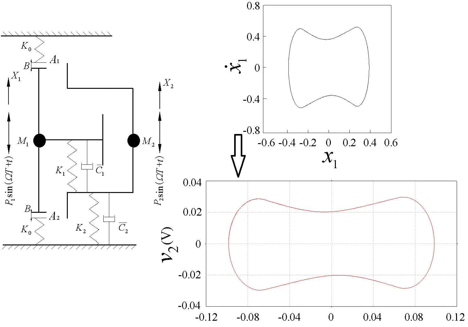
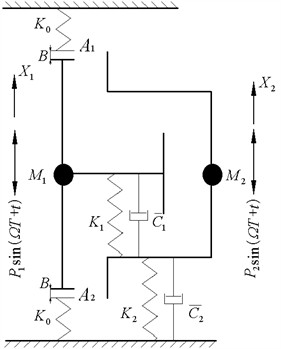
A two-degree-of-freedom vibration system with clearance composed of symmetric elastic stops is depicted in Fig.1. Although the model simplifies by excluding complex factors such as oil film forces and nonlinear stiffness, it holds significant qualitative value: the revealed dynamic patterns provide a theoretical foundation for understanding real-world systems. For instance, even in the presence of oil film forces, stiffness transitions and impacts induced by clearances remain key mechanisms for vibration amplification. Table 1 presents the definitions and units of the variables. The two oscillators with mass and are connected by a pair of linear spring-damping elements (, ), and another pair of elements (, ) couple the oscillator and the foundation. The harmonic excitation force acts on oscillator , where , and are the amplitude, excitation frequency and phase angle, respectively (). The coordinate system is established with the static equilibrium position of the system as the origin, and the displacements of the two oscillators are and , respectively. There are elastic constraints and with stiffness at the distance between the two sides of the oscillator . As the amplitude of the harmonic excitation is small, the system vibrates linearly, and the oscillator does not collide with the elastic constraints or . As the displacement of the oscillator is greater than the designed clearance threshold , i.e., , the impact event occurs in the system. Elastic constraints cause the systems with linear characteristics to exhibit complex non-smooth features.
The motion differential equation of the piecewise linear system in Fig. 1 is written as:
The piecewise linear spring force generated by the collision is given by:
In the present model, the contact interface is simplified as a constraint spring with stiffness . Future work could draw inspiration from the approach to bolted joint interfaces described in Ref. [34], describing the local nonlinear stiffness (e.g., Hertzian contact stiffness) in the clearance contact region as an “equivalent virtual material layer” that varies with contact state. This would facilitate the development of dynamic models that more accurately reflect the micro-mechanical properties of the interface.
Fig. 1Two-degree-of-freedom periodic forced vibration system with elastic constraints
The dimensionless parameters, time and variables are technically selected as:
then, the dimensionless expression of Eq. (1) is rewritten as:
in which, the expression of the spring force is:
3. Poincaré maps
For such harmonically excited systems featuring spring-damper cushioning mechanisms, the term “soft impact” is commonly used to characterize the collision behavior. Unlike rigid impact, rigid impact uses a discrete mapping of recovery coefficients to describe sudden changes in motion state, while soft impact considers the time effect of contact deformation during collision and typically uses piecewise functions to describe the non-smooth characteristics of the system. By varying the stiffness from zero to infinity within a specified interval, the system can transition from a piecewise linear model to a rigid impact model. The dynamic behaviors under these two limiting conditions have been thoroughly investigated in Refs. [35]. Various mathematical models corresponding to soft impact have been developed for different practical scenarios, such as the Kelvin-Voigt model in Refs. [36], the Hertz contact model in Refs. [37], and the piecewise linear model in Ref. [38].
Due to the existence of constraints, the system motion is separated into several subspaces, i.e., , and , in which, indicates that the oscillator collides with the constraint ; indicates that there is no collision between the oscillator and the elastic constraints (and ) on both sides; indicates that the oscillator collides with the lower elastic constraint , where, , .
The general solution of Eq. (4) is:
where, symbols , , are matrix elements corresponding to state paces , , , respectively. , , , , , . Symbols , and represent the undamped natural frequencies in three subspaces (, , ), respectively. Symbols , , and , , are amplitude constants in three subspaces (, , ), respectively. The integral constants , , and , , are determined by the initial conditions of the vibration system shown in Fig. 1. and .
We introduce the symbol to describe the basic characteristics of the periodic motion, where denotes the number of periods of the excitation force, and denote the number of impacts associated with the oscillator and the elastic constraints and on both sides, respectively (). In particular, for response with as well as , we call it symmetric single-period multi-impact motion.
Based on the meaning of the symbol , three Poincaré maps are defined:
Fixed points corresponding to section can determine the period number . Fixed points corresponding to and sections can respectively determine the number of collisions and of the oscillator at the upper () / lower () limiting constraints on both sides. The impact Poincaré map is briefly represented as:
where, , , . The symbol is the system parameter, which can be any of the system parameters, i.e., , , , , , , and .
The response -1-1 with -period and double-impact is likely to appear in the vibro-impact system with symmetric elastic constraints in Fig. 1. The characteristic of the response -1-1 lies in the fact that the instantaneous time after the collision between the oscillator and the elastic stop is zero, then the instantaneous time before the next impact is exactly . Periodicity conditions for symmetric -1-1 response are given as follows:
4. 1-p-p periodic motion and chattering-impact characteristic
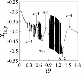
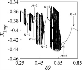
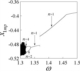
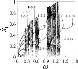
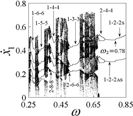
In this section, the variable-step fourth-order Runge-Kutta integration method is employed to numerically simulate the vibro-impact system with clearance shown in Fig. 1. To eliminate the influence of transient processes and ensure the reliability of the analysis, the transient responses from the first 500 periods were discarded, and the steady-state response data from the subsequent 30 periods were retained for analyzing the dynamics of the system. The 1-- response and chattering-impact characteristics are analyzed. The step size is 0.005 and the system parameters are fixed as 0.25, 0.0, 0.5, 0.5, 0.95, 0.5, 0.1. Figs. 2(a)-2(a2) intuitively show the dynamic response of the system with frequency in the range of by means of bifurcation diagrams and as well as Lyapunov exponent . Specifically, Figs. 2(a)-2(c) are bifurcation diagrams based on Poincaré mapping , where the number of branches in the curve determines the number of periods ; Figs. 2(a1)-2(c1) are bifurcation diagrams based on Poincaré mapping , where the number of branches in the curve determines the number of impacts between oscillator and upper constraint ; Figs. 2(a2)-2(c2) are the largest Lyapunov exponent corresponding to Figs. 2(a1)-2(c1). According to whether the Lyapunov exponent is greater than zero, the stability of the system can be effectively determined. Figs. 2(b)-2(c) are the detailed descriptions of local intervals in Fig. 2(a). Figs. 2(b1)-2(c1) are the detailed descriptions of Fig. 2(a1). Figs. 2(b2)-2(c2) are the detailed descriptions of Fig. 2(a2).
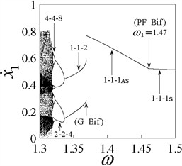
Symmetrical 1-1-1 motion is a typical dynamic response of the system with symmetric constraints, which usually occurs Pitchfork bifurcation. As shown in Fig. 2(c1), Pitchfork bifurcation (abbreviated as PF Bif in Fig. 2(c1)) causes the symmetric 1-1-1S response to transit to asymmetric response 1-1-1AS with the decrease of frequency (the subscript is the abbreviation for “symmetric”, and is the abbreviation for “asymmetric”). At the Pitchfork bifurcation point 1.47, the largest Lyapunov exponent is , as shown in Fig. 2(c2). Fig. 3(a) shows the phase plane portrait of the symmetric 1-1-1S response at before the Pitchfork bifurcation point, and Fig. 3(b) shows the phase plane portrait of the asymmetric 1-1-1AS response at 1.43 after Pitchfork bifurcation point. The asymmetric response 1-1-1AS presents two different forms of motion trajectories due to different initial values. The two are antisymmetric, such as the black and red motion trajectories in Fig. 3(b). As continues to decrease, the 1-1-1AS response transits to 1-1-2 through the Grazing bifurcation (abbreviated as G Bif in Fig. 2(c1)), and then the system enters chaos through the period-doubling cascade of the 1-1-2 response.
As continues to decrease, 1-2-2 response degenerates from chaotic response and again embeds chaos through the period-doubling cascade. Repeatedly, until the number of impacts increases to a large enough number, the system exhibits chattering-impact characteristics, which produces noise pollution, causing loose parts and fatigue, and even lead to machine parts fracture. This paper conducts an in-depth study on the low-frequency dynamics of the system with clearance in Fig. 1, laying a theoretical foundation for high-precision condition monitoring. It is noteworthy that the novel intelligent sensing structure provides a new approach to directly obtain high signal-to-noise ratio vibration responses [39]. By sensing the dynamic load of the bearing body, it can effectively capture rich dynamic behaviors such as impacts and bifurcations induced by clearance nonlinearity.
For small clearance, as frequency decreases, the transition law from symmetric response to chattering response is : 1-- ←…← 1-- ←chaos ←…← PD Bif ← 4-8-8 ← PD Bif ← 2-4-4 ← PD Bif ← 1-2-2 ← chaos ←… PD Bif ← 4-4-8 ← PD Bif ← 2-2-4 ← PD Bif ← 1-1-2 G Bif ← 1-1-1AS ← PF Bif ← 1-1-1Swhere, PF Bif indicates Pitchfork Bifurcation; G Bif indicates Grazing Bifurcation; PD Bif indicates Period-doubling Bifurcation.
Fig. 2Bifurcation diagrams x1min and x˙1(ω), and Lyapunov exponent diagram λmax, b= 0.25
a) Bifurcation diagram
b) Enlarged view 1 of Fig. 2(a)
c) Enlarged view 2 of Fig. 2(a)
a1) Bifurcation diagram
b1) Enlarged view 1 of Fig. 2(a1)
c1) Enlarged view 2 of Fig. 2(a1)
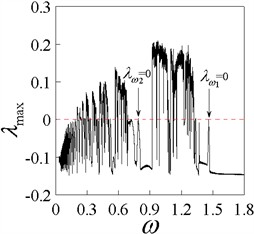
a2) Diagram
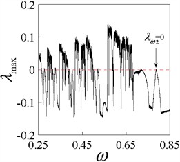
b2) Enlarged view 1 of Fig. 2(a2)
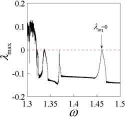
c2) Enlarged view 2 of Fig. 2(a2)
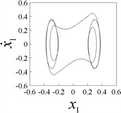
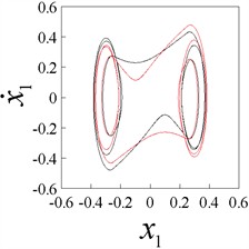
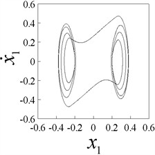
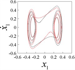
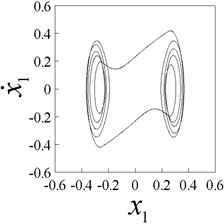
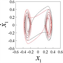
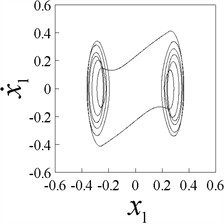
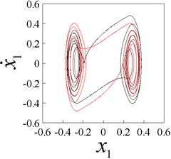
Fig. 3Phase plane portraits (x1,x˙1) of 1-p-p responses (p= 1-8), b= 0.25
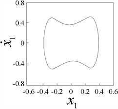
a) 1-1-1S, 1.55
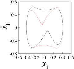
b) 1-1-1AS, 1.43
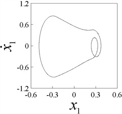
c) 1-1-2, 1.34
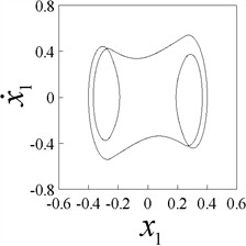
d) 1-2-2S, 0.85
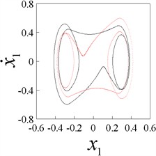
e) 1-2-2AS, 0.75
f) 1-3-3S, 0.54
g) 1-3-3AS, 0.515
h) 1-4-4S, 0.41
i) 1-4-4AS, 0.4
j) 1-5-5S, 0.335
k) 1-5-5AS, 0.32
l) 1-6-6S, 0.285
m) 1-6-6AS, 0.27
n) 1-7-7S, 0.24
o) 1-8-8S, 0.22
Figs. 3(a)-3(t) shows the phase plane portraits of 1-- (1-8) responses at different excitation frequencies. For 1-- response characterized by , there are also two antisymmetric trajectories due to different initial values, which are represented in black and red trajectories, respectively (see Fig. 3(g), Fig. 3(j), Fig. 3(m), Fig. 3(p), Fig. 3(r)).
The symmetric and asymmetric 1-- periodic motions discussed above are all verified by the equivalent electronic circuit designed in Section 4.
This study reveals the nonlinear dynamics induced by clearances under constant excitation. Future research will build upon the approach outlined in Ref. [40], extending into two key directions: transient process analysis and fault-coupled modeling.
5. Equivalent circuit model and simulation
5.1. Linear module design
In the previous section, the basic feature of 1-- response and chattering characteristics of the system with elastic constraints are analyzed through the use of bifurcation diagrams and phase portraits based on Poincaré mapping, as well as Lyapunov exponent. This method not only requires high programming ability, but also high-precision numerical simulation is limited by the operation performance of the computer, and the operation simulation speed is slow, which belongs to static calculation. As the system parameters are changed, the program needs to be recalculated, which takes up a large amount of computer capacity, consumes a lot of time and has poor economy. In this section, the equivalent electronic circuit model of the system shown in Fig. 1 is constructed using NI Multisim 14.0 software. Owing to its extensive component library and highly flexible parameter configuration capabilities, this software is particularly suitable for modeling vibration system circuits that involve nonlinear characteristics. The simulation method based on the equivalent circuit not only enables effective analysis of nonlinear dynamic behavior but also offers advantages such as high computational efficiency and the ability to dynamically adjust parameters.
In order to design the fully equivalent electronic circuit corresponding to the Eq. (1), the variable transformation , , , is introduced, and the Eq. (1) can be transformed into the following state equations by reducing the order:
in which, the piecewise linear spring force can be rewritten as:
In order to reduce the noise, the TL074CN integrated operational amplifier is selected here, and the integration circuit, addition circuit and amplification circuit composed of resistors, capacitors and other components are combined to realize Eq. (10). The schematic diagram of the designed electronic circuit is shown in Fig. 4, the structure of which is described as follows. Firstly, four integral operational amplifier circuits, i.e., , , and , are the main components of the circuit, which are expressed as integral treatment of four parameters, i.e., , , and , respectively; secondly, , , and are amplification circuits, which represent the reverse amplification of the four variables , , and , respectively; thirdly, and are integral summation circuits.
Fig. 4Linear circuit design diagram
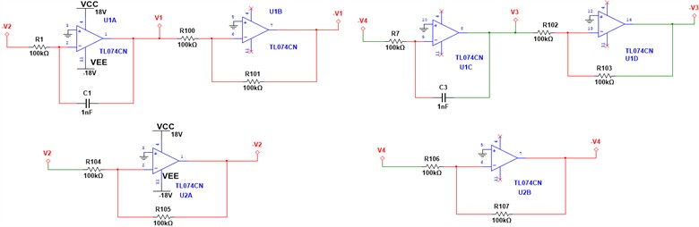
a) Integrating circuit
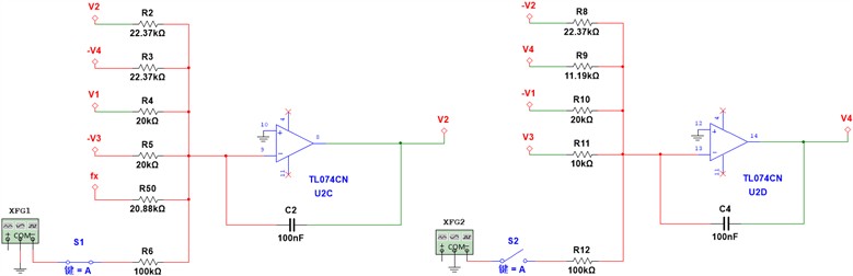
b) Summing amplifier
In order to determine the values of capacitors (, , and ) and resistors (, and ) of the circuit in Fig. 4, we introduce Kirchhoff's law and active electronic circuit, then, Eq. (10) can be transformed into the following circuit state space equations:
Transform Eq. (12) into the following second-order differential equations:
In order to make Eq. (1) and Eq. (10) completely equivalent, the following relationship should be satisfied:
The values of the resistors and capacitors in Fig. 4 are determined as follows. First, based on the dimensionless system parameters given in Section 4, i.e., , , , , , , , and by introducing state variables to transform Eq. (1) into state-space form, the initial component values are determined as 100 kΩ and 1 nF, 100 nF. Next, according to the proportional relationships of the coefficients in Eq. (19), the remaining resistor values are calculated as 22.37 kΩ, 20 kΩ, 11.19 kΩ, 10 kΩ, 20.88 kΩ. Finally, for the operational amplifiers , , and , which are used solely for signal inversion, the peripheral resistors are uniformly set as 100 kΩ.
According to the proportional relationship of coefficients , , , it can be concluded that the voltage amplitude of the sine signal is related to the clearance threshold . Therefore, we can obtain:
The correlation between the input frequency and the excitation frequency is:
i.e., .
5.2. Nonlinear module design
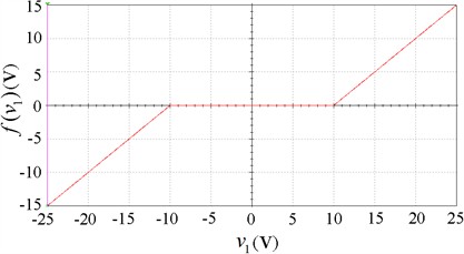
The nonlinear factor of the system is derived from the collision of the oscillator at the elastic constraints or , which is described by three linear functions, see Eq. (17):
where, .
Therefore, the linear saturation characteristics of the operational amplifier can be utilized to design the nonlinear circuit represented by Eq. (17). As shown in Fig. 5, the nonlinear circuit is composed of two circuit modules with the same magnification, opposite phase and different saturation parameters, which are linearly superimposed with the addition circuit. and are two in-phase operational amplifier units, and the output characteristic curves are shown in Fig. 6(a); is a reverse operational amplifier unit, and the output characteristic curve is shown in Fig. 6(b); is an additive operational amplifier unit. By utilizing the different saturation parameter intervals in Figs. 6(a)-6(b), Eq. (17) can be achieved through linear superposition of the additive operational amplifier unit , as shown in Fig. 6(c).
Fig. 5Non-linear circuit design diagram
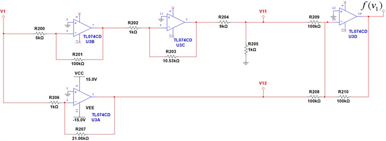
Fig. 6Piecewise linear function implementation diagram
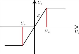
a) Phase amplification
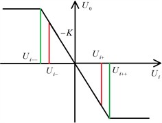
b) Reverse amplification
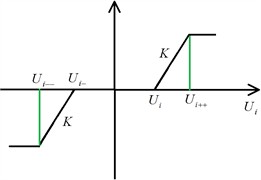
c) Superimposed output
The power supply voltage of the integrated operational amplifier TL074CN is selected as ±15 V, and the saturation voltage is selected as ±13 V. Then, we can obtain 5 kΩ, 100 kΩ, 1 kΩ, 10.53 kΩ, 9 kΩ, 1 kΩ, in which resistors and are used for voltage division. It can be calculated that the amplification factor of the forward amplifier circuit is 210.6, and the output is:
that is:
In order to make the inverter achieve saturation, the inverse magnification is 21.06, from which it can be inferred that 1 kΩ, 21.06 kΩ. Due to the fact that the saturated input voltage of is much higher than the actual input voltage of , only the majority of the output is taken, and the inverted output is , and . Finally, the sum of and is completed through the adder , and the inverted output can be obtained as follows ():
Based on the design of the nonlinear equivalent circuit in Eq. (20), the output characteristics of the piecewise linear function simulated in the MultiSim14.0 environment are shown in Fig. 7, where the abscissa is and the ordinate is .
Fig. 7Output characteristics of nonlinear circuit
5.3. MultiSim14.0 simulation
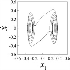
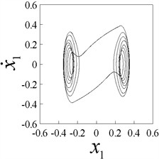
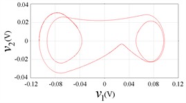
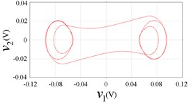
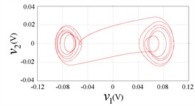
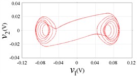
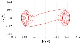
Fig. 8 is the circuit phase plane portraits simulated in MultiSim14.0 environment based on the equivalent circuit. The input voltage is 1.28 V and the input frequency is . We can observe that the simulation results obtained in MultiSim14.0 environment are in good agreement with the numerical simulation results in Fig. 3.
Fig. 8Circuit phase plane portraits, b= 0.25
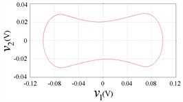
a) 1-1-1S, 554 Hz
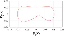
b) 1-1-1AS, 511 Hz
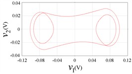
c) 1-2-2S, 304 Hz
d) 1-2-2AS, 268 Hz
e) 1-3-3S, 193 Hz
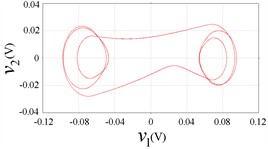
f) 1-3-3AS, 184 Hz
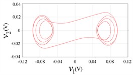
g) 1-4-4S, 146 Hz
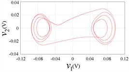
h) 1-4-4AS, 142 Hz
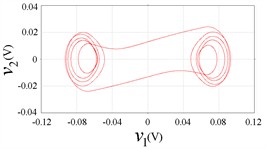
i) 1-5-5S, 120 Hz
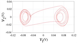
j) 1-5-5AS, 114 Hz
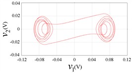
k) 1-6-6S, 102 Hz
l) 1-6-6AS, 96 Hz
m) 1-7-7S, 86 Hz
n) 1-8-8S, 78 Hz
In addition, symmetric and asymmetric 1-- responses, as well as periodic motions with large number of impacts, such as 1-7-7 and 1-8-8 responses, can be clearly captured. The test results demonstrate the advantages of the circuit simulation approach: on identical hardware, its computational time is only one-third of that required by conventional numerical solution methods, while entirely eliminating the cumbersome steps of modifying code and recompiling after parameter adjustments.
6. Conclusions
A combined approach of the fourth-order Runge-Kutta method and equivalent circuit simulation is utilized to explore the mechanisms of the 1-- response and chattering-impact phenomena in a two-degree-of-freedom vibro-impact system with elastic constraints.
1) In the case of small clearance, the system undergoes the following changes as changes from high to low: (i) symmetric 1-- response occurs Pitchfork bifurcation to produce asymmetric 1-- response, which has two antisymmetric trajectories due to different initial values; (ii) Asymmetric 1-- response is embedded into chaos through periodic-doubling bifurcation sequence; (iii) The system degenerates from chaotic to response; (4) as increases sufficiently, the system is characterized by chattering-impact response. However, 1-- response may undergo Grazing bifurcation, resulting in response.
2) Based on the mechanical model, an equivalent circuit model is built through the integral circuit, inverse circuit and addition circuit designed by common electronic components such as resistor, capacitor and integrated operational amplifier. The nonlinear circuit is designed by using the amplification and saturation characteristics of the operational amplifier. The numerical simulation output results obtained by fourth-order Runge-Kutta integration method are completely consistent with the circuit simulation output results. Compared with numerical simulation, especially high-precision numerical simulation algorithms, circuit simulation is not only fast, efficient, but also economical. It has low requirements on computer performance and can realize real-time adjustment of parameters. The dynamic characteristics of the system under different excitation frequencies and clearance thresholds can be obtained by changing the input frequency and voltage amplitude. The equivalent circuit simulation can be further extended to the dynamics analysis of mechanical systems with multiple-clearances and multiple-degrees-of-freedom, providing a novel and feasible reference idea and technical approach for the dynamic analysis of various mechanical devices involving nonlinear factors.
3) In the follow-up arrangement of the research content, we can engrave the hardware PCB circuit according to the designed electronic circuit schematic diagram, and realize the experimental verification of the hardware circuit for the vibration system with clearances. In the design and manufacturing of PCBs, the following issues need to be considered to ensure the stability and reliability of the circuit. For example, fully considering the clearance between components to prevent short circuits or series problems caused by too close spacing between components during the welding process; It is necessary to shorten the length of the wires as much as possible, avoid excessive through holes, and increase the difficulty of PCB soldering. In the field of mechanical engineering, Men et al. [41] successfully adapted simulated vibration data to real-world scenarios via style transfer technology to address the small-sample problem in bearing fault diagnosis, and their research paradigm is highly consistent with this work.
References
-
Y. Shi, G. Luo, and X. Lyu, “Multiformity and evolution characteristics of periodic motions in mechanical vibration systems with clearances,” Journal of Vibration Engineering and Technologies, Vol. 11, No. 8, pp. 3607–3625, Nov. 2022, https://doi.org/10.1007/s42417-022-00771-x
-
X. Lyu, Y. Shi, and G. Luo, “Two-parameter non-smooth bifurcations of period-one motions in a plastic impacting oscillator,” International Journal of Non-Linear Mechanics, Vol. 138, p. 103849, Jan. 2022, https://doi.org/10.1016/j.ijnonlinmec.2021.103849
-
D. Costa et al., “Chaos in impact oscillators not in vain: Dynamics of new mass excited oscillator,” Nonlinear Dynamics, Vol. 102, No. 2, pp. 835–861, May 2020, https://doi.org/10.1007/s11071-020-05644-0
-
Y. Liu, J. Páez Chávez, B. Guo, and R. Birler, “Bifurcation analysis of a vibro-impact experimental rig with two-sided constraint,” Meccanica, Vol. 55, No. 12, pp. 2505–2521, May 2020, https://doi.org/10.1007/s11012-020-01168-4
-
F. Luo and Z. Du, “Complicated periodic cascades arising from double grazing bifurcations in an impact oscillator with two rigid constraints,” Nonlinear Dynamics, Vol. 111, No. 15, pp. 13829–13852, Jun. 2023, https://doi.org/10.1007/s11071-023-08600-w
-
S. Yin, G. Wen, J. Ji, and H. Xu, “Novel two-parameter dynamics of impact oscillators near degenerate grazing points,” International Journal of Non-Linear Mechanics, Vol. 120, p. 103403, Apr. 2020, https://doi.org/10.1016/j.ijnonlinmec.2020.103403
-
R. Peng, Q. Li, and W. Zhang, “Homoclinic bifurcation analysis of a class of conveyor belt systems with dry friction and impact,” Chaos, Solitons and Fractals, Vol. 180, p. 114469, Mar. 2024, https://doi.org/10.1016/j.chaos.2024.114469
-
J. H. Xie, “A mathematical model for impact hammers and it’s global bifurcations,” Chinese Journal of Theoretical and Applied Mechanics, Vol. 29, No. 4, pp. 456–463, Aug. 1997.
-
G. Li, S. Wu, H. Wang, J. Sun, and W. Ding, “Global behavior of a simplified model for the micro-vibration molding machine in parameter-state space,” Mechanism and Machine Theory, Vol. 154, p. 104039, Dec. 2020, https://doi.org/10.1016/j.mechmachtheory.2020.104039
-
J. Xie and W. Ding, “Hopf-Hopf bifurcation and invariant torus of a vibro-impact system,” International Journal of Non-Linear Mechanics, Vol. 40, No. 4, pp. 531–543, May 2005, https://doi.org/10.1016/j.ijnonlinmec.2004.07.015
-
P. Krasilnikov, T. Gurina, and V. Svetlova, “Bifurcation study of a chaotic model variable-length pendulum on a vibrating base,” International Journal of Non-Linear Mechanics, Vol. 105, pp. 88–98, Oct. 2018, https://doi.org/10.1016/j.ijnonlinmec.2018.06.011
-
J. Cao and J. Fan, “Discontinuous dynamical behaviors in a 2-DOF friction collision system with asymmetric damping,” Chaos, Solitons and Fractals, Vol. 142, p. 110405, Jan. 2021, https://doi.org/10.1016/j.chaos.2020.110405
-
Y. Yue and J. Xie, “Neimark-Sacker-pitchfork bifurcation of the symmetric period fixed point of the Poincaré map in a three-degree-of-freedom vibro-impact system,” International Journal of Non-Linear Mechanics, Vol. 48, pp. 51–58, Jan. 2013, https://doi.org/10.1016/j.ijnonlinmec.2012.07.002
-
X.-F. Gou, L.-Y. Zhu, and D.-L. Chen, “Bifurcation and chaos analysis of spur gear pair in two-parameter plane,” Nonlinear Dynamics, Vol. 79, No. 3, pp. 2225–2235, Nov. 2014, https://doi.org/10.1007/s11071-014-1807-1
-
Y. Zhang and G. Luo, “Multistability of a three-degree-of-freedom vibro-impact system,” Communications in Nonlinear Science and Numerical Simulation, Vol. 57, pp. 331–341, Apr. 2018, https://doi.org/10.1016/j.cnsns.2017.10.007
-
J.-F. Shi, X.-F. Gou, and L.-Y. Zhu, “Modeling and analysis of a spur gear pair considering multi-state mesh with time-varying parameters and backlash,” Mechanism and Machine Theory, Vol. 134, pp. 582–603, Apr. 2019, https://doi.org/10.1016/j.mechmachtheory.2019.01.018
-
S. Deng, J. Ji, G. Wen, and H. Xu, “Two-parameter dynamics of an autonomous mechanical governor system with time delay,” Nonlinear Dynamics, Vol. 107, No. 1, pp. 641–663, Nov. 2021, https://doi.org/10.1007/s11071-021-07039-1
-
Z. Tan, S. Yin, G. Wen, Z. Pan, and X. Wu, “Near-grazing bifurcations and deep reinforcement learning control of an impact oscillator with elastic constraints,” Meccanica, Vol. 58, No. 2-3, pp. 337–356, Jan. 2022, https://doi.org/10.1007/s11012-022-01475-y
-
Y. Sun, Z. He, J. Xu, W. Sun, and G. Lin, “Dynamic analysis and vibration control for a maglev vehicle-guideway coupling system with experimental verification,” Mechanical Systems and Signal Processing, Vol. 188, p. 109954, Apr. 2023, https://doi.org/10.1016/j.ymssp.2022.109954
-
G. W. Luo, Y. Q. Shi, C. X. Jiang, and L. Y. Zhao, “Diversity evolution and parameter matching of periodic-impact motions of a periodically forced system with a clearance,” Nonlinear Dynamics, Vol. 78, No. 4, pp. 2577–2604, Aug. 2014, https://doi.org/10.1007/s11071-014-1611-y
-
X. Lyu, J. Bai, and X. Yang, “Bifurcation analysis of period-1 attractors in a soft impacting oscillator,” Nonlinear Dynamics, Vol. 111, No. 13, pp. 12081–12100, Apr. 2023, https://doi.org/10.1007/s11071-023-08486-8
-
Y. Shi and J. Yang, “Diversity and transition of periodic motion of a periodically excited soft-impacting machinery,” Physica Scripta, Vol. 99, No. 10, p. 105273, Oct. 2024, https://doi.org/10.1088/1402-4896/ad7914
-
X. Lyu, X. Zhu, Q. Gao, and G. Luo, “Two-parameter bifurcations of an impact system under different damping conditions,” Chaos, Solitons and Fractals, Vol. 138, p. 109972, Sep. 2020, https://doi.org/10.1016/j.chaos.2020.109972
-
X. Lyu, Q. Gao, and G. Luo, “Dynamic characteristics of a mechanical impact oscillator with a clearance,” International Journal of Mechanical Sciences, Vol. 178, p. 105605, Jul. 2020, https://doi.org/10.1016/j.ijmecsci.2020.105605
-
G. W. Luo, Y. Q. Shi, X. F. Zhu, and S. S. Du, “Hunting patterns and bifurcation characteristics of a three-axle locomotive bogie system in the presence of the flange contact nonlinearity,” International Journal of Mechanical Sciences, Vol. 136, pp. 321–338, Feb. 2018, https://doi.org/10.1016/j.ijmecsci.2017.12.022
-
O. M. Njimah, J. Ramadoss, A. N. K. Telem, J. Kengne, and K. Rajagopal, “Coexisting oscillations and four-scroll chaotic attractors in a pair of coupled memristor-based Duffing oscillators: theoretical analysis and circuit simulation,” Chaos, Solitons and Fractals, Vol. 166, p. 112983, Jan. 2023, https://doi.org/10.1016/j.chaos.2022.112983
-
Z. Wang, C. Zhang, and Q. Bi, “Bursting oscillations with bifurcations of chaotic attractors in a modified Chua’s circuit,” Chaos, Solitons and Fractals, Vol. 165, p. 112788, Dec. 2022, https://doi.org/10.1016/j.chaos.2022.112788
-
Z. Wang, C. Zhang, and Q. Bi, “Bursting oscillations with adding-sliding structures in a Filippov-type Chua’s circuit,” Communications in Nonlinear Science and Numerical Simulation, Vol. 110, p. 106368, Jul. 2022, https://doi.org/10.1016/j.cnsns.2022.106368
-
G. A. Leonov and N. V. Kuznetsov, “Hidden attractors in dynamical systems: from hidden oscillations in Hilbert-Kolmogorov, Aizerman, and Kalman problems to hidden chaotic attractor in Chua circuits,” International Journal of Bifurcation and Chaos, Vol. 23, No. 1, p. 13300, Nov. 2013, https://doi.org/10.1142/s0218127413300024
-
K. Srinivasan, K. Thamilmaran, and A. Venkatesan, “Effect of nonsinusoidal periodic forces in Duffing oscillator: Numerical and analog simulation studies,” Chaos, Solitons and Fractals, Vol. 40, No. 1, pp. 319–330, Apr. 2009, https://doi.org/10.1016/j.chaos.2007.07.090
-
R. Balamurali, L. K. Kengne, K. Rajagopal, and J. Kengne, “Coupled non-oscillatory duffing oscillators: multistability, multiscroll chaos generation and circuit realization,” Physica A: Statistical Mechanics and its Applications, Vol. 607, p. 12817, Dec. 2022, https://doi.org/10.1016/j.physa.2022.128174
-
J.-H. Ho, V.-D. Nguyen, and K.-C. Woo, “Nonlinear dynamics of a new electro-vibro-impact system,” Nonlinear Dynamics, Vol. 63, No. 1-2, pp. 35–49, Aug. 2010, https://doi.org/10.1007/s11071-010-9783-6
-
M. Sekikawa, N. Inaba, T. Tsubouchi, and K. Aihara, “Novel bifurcation structure generated in piecewise-linear three-LC resonant circuit and its Lyapunov analysis,” Physica D: Nonlinear Phenomena, Vol. 241, No. 14, pp. 1169–1178, Jul. 2012, https://doi.org/10.1016/j.physd.2012.03.011
-
Z. Qin, L. Qin, Q. Zhu, P. Wang, F. Zhang, and F. Chu, “An ultrasensitive self-powered smart bearing pedestal with fault locating capability,” Mechanical Systems and Signal Processing, Vol. 235, p. 112924, Jul. 2025, https://doi.org/10.1016/j.ymssp.2025.112924
-
M. Pascal, “Dynamics and stability of a two degree of freedom oscillator with an elastic stop,” Journal of Computational and Nonlinear Dynamics, Vol. 1, No. 1, pp. 94–102, Jan. 2006, https://doi.org/10.1115/1.1961873
-
K. H. Hunt and F. R. E. Crossley, “Coefficient of restitution interpreted as damping in vibroimpact,” Journal of Applied Mechanics, Vol. 42, No. 2, pp. 440–445, Jun. 1975, https://doi.org/10.1115/1.3423596
-
J. Páez Chávez, E. Pavlovskaia, and M. Wiercigroch, “Bifurcation analysis of a piecewise-linear impact oscillator with drift,” Nonlinear Dynamics, Vol. 77, No. 1-2, pp. 213–227, Feb. 2014, https://doi.org/10.1007/s11071-014-1285-5
-
S. Kundu, S. Banerjee, J. Ing, E. Pavlovskaia, and M. Wiercigroch, “Singularities in soft-impacting systems,” Physica D: Nonlinear Phenomena, Vol. 241, No. 5, pp. 553–565, Mar. 2012, https://doi.org/10.1016/j.physd.2011.11.014
-
D. Du, Y. Tian, W. Sun, H. Liu, X. Liu, and H. Zhang, “Semi-analytical dynamic modeling and vibration analysis of double cylindrical shell structure based on the general bolted flange model,” Engineering Structures, Vol. 333, p. 120027, Jun. 2025, https://doi.org/10.1016/j.engstruct.2025.120027
-
B. Yang, Y. Li, C. Wen, L. Li, B. Li, and W. Song, “Rub-impact investigation on the lateral-torsional coupled vibration of a bolted joint rotor system with interface contact,” Applied Mathematical Modelling, Vol. 151, p. 116459, Mar. 2026, https://doi.org/10.1016/j.apm.2025.116459
-
Z. Men, D. Gong, K. Zhou, Y. Chen, and J. Zhou, “Unsupervised domain adaptation method for bearing fault diagnosis assisted by twin data under extreme sample scarcity,” Mechanical Systems and Signal Processing, Vol. 239, p. 113359, Oct. 2025, https://doi.org/10.1016/j.ymssp.2025.113359
About this article

This work was supported by Technology and Equipment of Rail Transit Operation and Maintenance Key Laboratory of Sichuan Province [2024YW005]; Science and Technology Plan Projects of Gansu Province [25JRRA162].
The datasets generated during and/or analyzed during the current study are available from the corresponding author on reasonable request.
Yuqing Shi: conceptualization, investigation, methodology, writing-original draft, writing-review and editing, validation, formal analysis, funding acquisition. Longfei He: supervision, project administration, data curation.
The authors declare that they have no conflict of interest.
