Abstract
This study proposes a comprehensive framework for automated diagnostics of rotating machinery using vibration signals. The methodology integrates the stages of dataset selection and preparation, signal processing, feature extraction, dimensionality reduction and training and testing of supervised machine learning algorithms. The preparation of the dataset involves proposing a technique for addressing data imbalance, normalisation of the data amplitude, adjusting the sampling frequency, and calculating the actual rotational frequency. Then, appropriate signal filters are designed and applied, and a wide range of statistical and spectral features is extracted in the time and frequency domain. To address the challenges of high-dimensional feature spaces and allow transparency in identifying features with the highest level of importance in recognising machinery faults, a group-wise dimensionality reduction technique, Sequential Selection Algorithm (SSA), is proposed. The applicability of the proposed SSA technique is validated by comparing its performance with that of commonly used dimensionality reduction techniques, by testing its compatibility with supervised machine learning algorithms, and by analyzing its efficiency. In that sense, a set of models combining four dimensionality reduction techniques and four supervised machine learning algorithms is trained and tested, and their accuracy is compared.
Highlights
- A comprehensive framework for automated vibration-based fault diagnostics of rotating machinery is developed.
- A group-wise Sequential Selection Algorithm (SSA) is proposed for interpretable dimensionality reduction.
- The SSA-SVM model achieves 97.06% classification accuracy using only 29 input features.
- SSA reduces feature-selection time by 94.2% compared with conventional Sequential Forward Selection (SFS).
- The proposed framework enables substantial computational savings while preserving high diagnostic accuracy.
1. Introduction
Modern rotating machinery is required to operate at higher speeds and deliver greater productivity while maintaining high product quality. as these performance requirements grow, the maintenance process becomes more demanding, and its associated costs rise substantially. for example, 15 to 40 % of the total costs for producing a product in systems composed of rotating machinery are due to maintenance costs [1]. in order to overcome these challenges, various maintenance strategies have been developed and implemented in modern production systems. Among them, condition-based maintenance (CBM) has been one of the most widely adopted approaches, which monitors the machinery state based on parameters highly sensitive to mechanical changes and fault development [2, 3]. in this regard, vibration is considered the most reliable indicator, as it enables fault detection at the earliest stages of its progression [4-8].
Vibration signals, measured in the time domain using vibration transducers, contain valuable information related to the condition of various machine components, as well as some background noise. Consequently, before the diagnostics process, signal preprocessing is required to suppress noise and emphasise fault-related information in the raw vibration signals. To apply the condition-based maintenance strategy to complex machinery systems, it is essential to minimise the time required for signal processing and fault identification. One way to address this issue is through the automation of the condition monitoring process [9, 10]. As a result, subjectivity and potential human error in the decision-making process can be substantially reduced, thereby improving reliability and consistency in diagnostics. Such automation can be realised through different approaches, including physics-based models, data-driven models, or a hybrid combination of both. A significant research interest has been devoted to the optimisation of traditional maintenance strategies by integrating artificial intelligence (AI), advanced learning techniques, large datasets, and high-performance computing [11-13].
Recently, the application of machine learning algorithms for vibration-based fault diagnostics of rotating machinery has attracted considerable research attention. Das et al. [14] published a comprehensive review of intelligent fault diagnosis and prognosis strategies for rotating machinery, emphasising the challenges that remain in practical application. Latil et al. [15] provided a review and bibliometric analysis of supervised approaches that have shown the best performance under varying working conditions. Due to the ability to capture discriminative patterns from labelled datasets and accurately classify machine conditions, the supervised learning methods have been widely adopted. A key advantage of supervised machine learning is that high diagnostic accuracy and efficiency can be achieved without requiring huge datasets, which is especially relevant since most available vibration datasets are of moderate size [16-18]. Once trained, these models can deliver fast predictions, which makes them applicable for real-time fault monitoring in smart factories. Additionally, their effectiveness and accuracy strongly depend on the quality of the features extracted from the measured vibration signals. Therefore, feature extraction is a crucial step which converts preprocessed data into compact and informative classification inputs. At the same time, using high-dimensional input vectors is not always beneficial, as they may introduce redundancy and noise, increase computational complexity, and lead to overfitting [19-21]. To enhance accuracy and generalisation by allowing the model to learn from the most significant information, dimensionality reduction techniques are applied.
There are many challenges in this field which are associated with noisy vibration data in the measured signals and high dimensionality of the input vectors. in response to these challenges, numerous studies have proposed and tested advanced techniques for signal analysis and feature extraction to obtain compact and informative inputs. Brito et al. [22] highlighted the risks associated with using high-dimensional input vectors and emphasised the value of using significant and concise feature vectors. Neupane et al. [23] and Tiboni et al. [24] showed that signal processing and feature selection techniques strongly affect the accuracy of the automated model for condition monitoring of rotating machinery.
Depending on the extracted features and the specific fault types analysed, the choice of algorithms can significantly impact diagnostic accuracy. Therefore, the existing state-of-the-art in this field evaluates a wide range of supervised machine learning algorithms for vibration-based fault classification. for example, Pelayo-González et al. [25] demonstrated that a combination of envelope analysis, a minimal feature set and k-Nearest Neighbours (k-NN) and decision tree algorithms, can result in an accuracy of up to 100 %. They classified rolling bearing faults using the Case Western Reserve University (CWRU) dataset. Zhang et al. [26] significantly increased the diagnostic accuracy and efficiency of the proposed model using an adequate combination of a dimensionality reduction technique and Support Vector Machine (SVM) algorithm. Complementing these results, Wang et al. [27] proposed a robust methodology which integrates variational mode decomposition (VMD) and nonlinear dimensionality reduction (t-SNE) techniques, and SVM algorithm. Their approach achieved a high diagnostic accuracy of 96 %-99.7 % and computational efficiency in classifying bearing faults when tested with multiple datasets. Singh et al. [28] proposed a graph-based fault diagnosis methodology which achieved up to 100 % accuracy on the CWRU and Southeast University (SU) datasets. The results showed that Random Forest (RF) significantly outperformed SVM and logistic regression. Shen et al. [29] reached an accuracy of 100 % in classifying inner race, outer race, and ball bearing faults by using an improved grey wolf algorithm (IGWO) to optimise the SVM algorithm.
While the authors in [27-30] have focused on the classification of rolling bearing faults, several other works have addressed another group of fault types, in particular, imbalance and misalignment [31-34]. Dineva et al. [31] applied a multi-label classification framework to classify imbalance and misalignment faults. Zhou et al. [32] used SVM and decision trees algorithms to classify imbalance and angular misalignment using vibration signals measured on an experimental rotating machinery test rig. Cao et al. [33] classified imbalance and misalignment faults during steady-state conditions, and achieved high accuracy in classification using optimised feature selection techniques. Rezazadeh et al. [34] compared SVM, k-NN, and Naive Bayes accuracy for the classification of imbalance, cracks, and misalignment during steady-state conditions.
While these examples focused on fault classification between distinct groups of faults, other studies considered a wider range of fault types. Atmaja et al. [35] proved the effectiveness of supervised learning techniques for classifying bearing faults, imbalance, and misalignment under constant load, achieving an accuracy of 99.75 %. Huynh and Min [36] used SVM and achieved 99.80% accuracy in classifying ten fault conditions: imbalance, misalignment, and various bearing faults, at a constant rotational speed. They also mentioned that the accuracy remained at 99.70 % after reducing the dimension of the input feature set and that it reduced the training time considerably. Li et al. [37] proposed a relevant method for industrial applications, based on domain adaptation and SVM, and improved diagnostic performance under variable load conditions. Patel and Upadhyay [38] compared the accuracy of SVM, k-NN, and decision trees algorithms and confirmed the strong diagnostic potential of traditional supervised classifiers in detecting machinery faults. Ovacikli et al. [39] trained and tested the accuracy of RF, k-NN, and SVM using various parameters, including vibration, temperature, and acoustic data.
Most of these approaches demonstrate the effectiveness of supervised learning algorithms that have been trained and tested using data measured under constant operating conditions. Although the obtained accuracies are high, their applicability in industrial settings is limited because, as noted in [15], real machinery rarely operates at constant loads and speeds. in addition, existing studies often restrict their scope to specific fault types, concentrating either on bearing faults [27-30] or on imbalance and misalignment [31-34], without addressing the challenge of classifying diverse fault categories. One of the main challenges in diagnosing faults of diverse categories under varying load conditions is the requirement for a higher sampling frequency to capture the characteristic frequencies associated with the analysed faults. for example, according to the Nyquist-Shannon sampling theorem [40, 41], the required sampling frequency increases if the classifier is supposed to recognise rolling bearing faults at high rotational speeds. Another challenge concerns the selection of an appropriate frequency band during signal preprocessing, as a broader range of frequencies must be retained for the algorithm to identify faults of different natures reliably. One way to address this issue is to design a measurement system that captures the maximum frequency of interest. Another approach is to use the desired value for the sampling frequency when measuring the signals and then reduce it adequately. If the second approach is chosen, suitable signal processing methods are essential to prevent signal distortion and leakage.
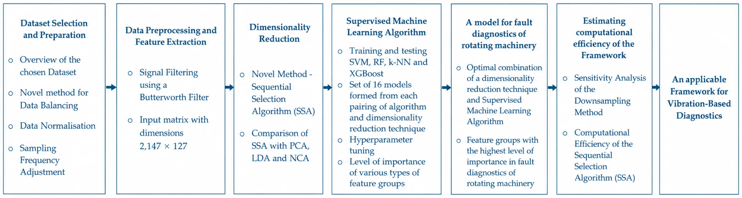
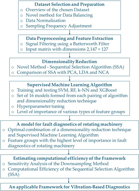
There are several challenges in implementing the proposed methodologies of the reviewed literature in real industrial applications. Firstly, industrial machines are often subject to diverse faults that manifest under varying operating conditions. Another critical issue is that, in practice, the distribution of measured signals of these faults in many datasets is highly unbalanced, leading to the problem of class imbalance [42, 43]. in an imbalanced dataset, some classes are significantly underrepresented, which can bias the learning process and reduce diagnostic reliability. However, solving the issue of class imbalance has received limited attention within the framework of supervised learning methods. Moreover, the importance of different types of features in distinguishing different faults is seldom systematically evaluated, and therefore transparency regarding the most influential features is rarely achieved. To address these limitations, this study proposes a comprehensive diagnostic framework for diagnosis of a broader variety of fault types, under varying load conditions. The proposed framework in Fig. 1, integrates the phases of data set preparation, preprocessing, feature extraction, and training and testing of supervised algorithms.
More specifically, the proposed framework, shown in Fig. 1, follows the steps listed below, which structure the research process adopted in this study:
(i) Selection and systematic preparation of the Machinery Fault Database. This phase includes a novel method for data balancing to ensure more robust, unbiased, and generalizable diagnostic performance for real industrial applications. Furthermore, the stages of normalisation, adjustment of the sampling frequency, and calculation of the actual rotational frequency followed;
(ii) Signal preprocessing using suitable filtering. the preprocessed signals are obtained by applying an appropriately designed Butterworth high-pass filter;
(iii) Extraction of a comprehensive set of features. A wide range of time-domain, frequency-domain, and spectral features is extracted, resulting in a structured input feature matrix.
(iv) Dimensionality reduction of the input feature matrix. To provide complete transparency in assessing the influence of different feature categories, a group-wise dimensionality reduction technique, the Sequential Selection Algorithm (SSA), is proposed.
(v) Designing a comprehensive set of diagnostic models. The applicability of the proposed SSA technique is validated by comparing its performance with that of commonly used dimensionality reduction techniques, by testing its compatibility with supervised machine learning algorithms, and by analyzing its efficiency. in this context, four dimensionality reduction techniques are combined with four supervised learning algorithms. More specifically, three standard dimensionality reduction techniques are used such as Principal Component Analysis (PCA), Linear Discriminant Analysis (LDA), and Neighbourhood Component Analysis (NCA), and the group-wise SSA technique. Also, four supervised learning algorithms are used such as Support Vector Machines (SVM), k-Nearest Neighbors (k-NN), Random Forests (RF) and Gradient Boosting (XGBoost). All models are trained and tested in a systematic manner, and their diagnostic accuracy is compared.
(vi) Evaluation of the diagnostic accuracy. Model performance is assessed using a 10-fold cross-validation technique and a confusion matrix, which allow analysis of both overall and per-class accuracy;
(vii) Estimation of the computational efficiency of the framework. The efficiency of the framework is quantified through a sensitivity analysis of the proposed downsampling method and by analysing the reduction in training and testing time which is achieved after applying the SSA technique.
(viii) Formulation of an applicable vibration-based diagnostic framework. Based on the previous steps, an applicable framework is obtained for diagnostics of a broader variety of fault types, including imbalance, vertical and horizontal misalignment, and bearing faults, under varying load conditions.
It is important to emphasise that the proposed diagnostic framework operates on a multivariate feature space, in which all extracted time, frequency, and spectral-domain features are analysed simultaneously. The dimensionality reduction techniques applied in this paper (PCA, LDA, NCA, and the proposed SSA) explicitly exploit correlations and interactions between features, ensuring that the intrinsic multivariate structure of the vibration data is preserved. Likewise, the supervised machine learning classifiers are trained on multidimensional input vectors, enabling them to learn nonlinear relationships among feature groups and capture complex fault-related patterns. Therefore, the entire workflow inherently incorporates multivariate analysis, both in feature selection and in model training.
In recent years, deep learning approaches, particularly one-dimensional convolutional neural networks (1D CNNs) [44-47] which operate directly on raw vibration signals, and transformer-based sequence models [48, 49] have demonstrated strong performance in vibration-based fault diagnostics. More recently, advanced architectures such as trustworthy lightweight multi-expert wavelet transformers [50], entropy-oriented semi-supervised dynamic prototype contrastive learning frameworks [51], and spatial-channel collaborative multi-scale graph interaction transfer learning methods [52] have further improved diagnostic robustness, transferability, and performance under limited labelled data conditions. These models are capable of automatically learning discriminative representations without requiring manually extracted features. However, such approaches generally require large datasets, complex network architectures, substantial computational resources, and often provide limited interpretability, which constrains their application in real industrial settings. in contrast, many industrial environments operate with moderate dataset sizes, strict real-time requirements, and the need for transparent and explainable diagnostic indicators. for these reasons, this study focuses on an interpretable and computationally efficient supervised machine learning framework, while acknowledging deep learning as an important direction for future research.
The paper is structured as follows: Chapter 2 provides an overview of the dataset and outlines the steps for its preparation, with a focus on the proposed novel method for data balancing. Chapter 3 outlines the methodology for signal preprocessing, which involves designing and applying suitable filters, as well as creating an input matrix of extracted features. The development of a group-wise dimensionality reduction method and its validation are shown in the first part of Chapter 4. The second part covers the training, testing, and optimisation phases of supervised machine learning algorithms and presents the results obtained regarding the optimal combination of a dimensionality reduction technique and a supervised machine learning algorithm. Chapter 5 introduces an efficiency analysis of the proposed framework, including a sensitivity study on the downsampling strategy and a detailed evaluation of the computational benefits achieved using the Sequential Selection Algorithm (SSA). Chapter 6 highlights the drawn conclusions and discusses the steps for future work and possible improvements to the proposed framework.
Fig. 1A proposed framework for automated fault diagnostics of rotating machinery
2. Dataset description and preparation
A dataset measured on a specific type of rotating machine may not generalise to other machine types or operating conditions. Therefore, it is essential to select a database for model training that accurately reflects the conditions under which the analysed machine system is expected to operate. The sampling frequency also plays a critical role in diagnostic accuracy, as it must be sufficiently high to capture the characteristic frequencies associated with the defects of interest. in addition, the effectiveness of supervised machine learning algorithms depends on using datasets in which signals are consistently annotated with their corresponding fault conditions. Inconsistent or incomplete labelling of the dataset can significantly reduce the efficiency and accuracy of the developed models. Additionally, proper dataset preparation is crucial in producing adequate data which is suitable for reliable preprocessing, feature extraction, and subsequent fault classification.
2.1. Dataset overview
Common faults in rotating machinery include imbalance, misalignment, rub, looseness, bearing faults, and gear defects [1]. Consequently, in this paper, the open-source Machinery Fault Database [53] was chosen for training and testing the proposed automated fault diagnostics system. The dataset was created by researchers at the Signals, Multimedia, and Telecommunication Laboratory, using the SpectraQuest Machinery Fault Simulator [54] as the experimental platform shown in Fig. 2. It has been documented in several studies, which describe its structure and emphasise its use in classifying faults in rotating machinery [55, 56]. The vibration signals from the selected dataset were acquired on the SpectraQuest Machinery Fault Simulator [54], which is a widely used laboratory test rig designed for controlled generation of common rotating machinery faults. The simulator consists of an electric motor, a shaft with two rotors which is supported by two bearings. The technical specifications of the simulator are shown in Table 1 and the technical specifications of the used accelerometers are shown in Table 2.
The database contains 1951 data files, making it one of the most extensive open-source vibration datasets available online. The signals were recorded under controlled experimental conditions, in the presence of several simulated fault conditions such as imbalance, misalignment, and rolling bearing defects. The speed of the actuation electromotor was regulated to enable testing under varying load conditions, and the rotational speed of the shaft was measured with a magnetic proximity sensor, which served as a tachometer. Vibration data were acquired along three axes, using three single-axis accelerometers mounted on the underhang bearing and one triaxial accelerometer mounted on the overhang bearing. A microphone was also used to record the acoustic response of the machine, but only vibration signals are considered in this study. All sensors were connected to the acquisition board, which converted the analogue signals into digital form for further processing.
Fig. 2Measurement setup for creating the machinery fault database [48, 50, 51]
![Measurement setup for creating the machinery fault database [48, 50, 51]](https://static-01.extrica.com/articles/25912/25912-img2.jpg)
The authors [55, 56] configured the acquired signals using NI LabVIEW software and stored them in text file format. Proper organisation of the data is essential to facilitate efficient processing, analysis, and development of intelligent systems for automatic fault detection. Six operating conditions were simulated: normal, imbalance, vertical misalignment, horizontal misalignment, faulty underhang bearing, and faulty overhang bearing. Each measurement was performed over a duration of 5 seconds at a sampling frequency of 50 kHz, resulting in 250,000 samples per signal. for each fault type, tests covered multiple fault severity levels and a range of rotational speeds from 11.7 to 60 Hz.
Table 1Technical specifications of SpectraQuest machinery fault simulator [54]
Parameter | Value | Unit |
Power of DC motor | 1/4 | HP |
RPM range of shaft | 700-3600 | rpm |
Weight | 22 | kg |
Diameter of rotors | 152,4 | mm |
Diameter of shaft | 16 | mm |
Lenght of shaft | 520 | mm |
Distance between bearings | 390 | mm |
Technical Specification of rolling bearings | ||
Number of balls | 8 | |
Ball diameter | 7,145 | mm |
Cage diameter | 28,519 | mm |
Pitch diameter () | 21,374 | mm |
Contact Angle | 41,5 | ° |
Table 2Technical specifications of accelerometers for creating the machinery fault database [48]
Parameter | Accelerometers on overhang bearing | Accelerometer on underhang bearing |
Model | Three industrial IMI 601A01 | One triaxial IMI 604B31 |
Sensibility | 100 mV/g ±20% 10,2 mV / (m/s2 )±20 % | 100 mV/g ±20 % 10.2 mV / (m/s2 )±20 % |
Frequency range | 0,27-10.000 Hz ±3 dB | 0,5-5.000 Hz ±3 dB |
Measurement range | ±50 g (±490 m/s2) | ±50 g (±490 m/s2) |
2.2. Addressing dataset imbalance
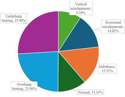
An imbalanced dataset can bias the training process of a supervised machine learning algorithm towards dominant classes. As a result, the detection of underrepresented classes can be compromised, reducing the overall accuracy of the classifier. A dataset can be classified as imbalanced if the number of samples in one class is less than 50 % of the average number of samples in the remaining classes [57]. Fig. 3 shows the percentage distribution of the number of signals in the dataset measured in each machinery state. It is evident that the signals measured in the normal operating condition are particularly underrepresented. There are only 49 signals in the normal state, compared to the calculated threshold value of 190.2, as defined in [57].
Fig. 3Percentage of signals recorded in the presence of each of the faults in the machinery fault database – before data balancing
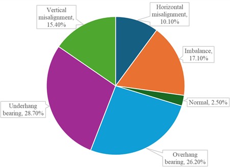
This means that the normal condition has less than half the average number of signals recorded in the presence of the faulty conditions. To achieve balance, at least 191 signals measured in normal condition are needed. Such an imbalance may reduce the accuracy in detecting normal operating state of the machine and increase the likelihood of false alarms.
To address these issues, a novel strategy for balancing the dataset is proposed to address the underrepresentation of signals measured under normal operating conditions in the dataset.
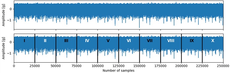
The original sampling frequency with a value of 50 kHz was reduced by a factor of 10, resulting in a new sampling frequency of 5 kHz. Consequently, the original signal, which consisted of 250,000 samples and was recorded over 5 seconds, was separated into 10 signals consisting of 25,000 samples each, recorded over the same time interval, Fig. 4. Every second signal was saved as a separate file, and the remaining five signals were discarded.
This process increased the number of files in normal condition from 49 to 245 and consequently increased the total number of files to 2,147 across all classes. Notably, this adjustment did not compromise diagnostic reliability, as signals recorded under normal operation do not contain fault-specific frequency components that are at risk of being lost. After balancing the dataset, the normal class accounted for 11.41 % of the dataset (compared to 2.5 % initially), resulting in a substantially more even class distribution, which can be seen from Fig. 5. Two additional aspects were considered to ensure data consistency and quality. First, the reduced sampling frequency with a value of 5 kHz was standardised across all classes. in this way, uniformity in the dataset and compatibility with the sensor-acquisition system setup is ensured. Second, an anti-aliasing filter was applied after decreasing the sampling frequency to prevent signal distortion and preserve essential fault-related frequency content. These aspects will be discussed in detail in the following chapters.
Fig. 4Balancing methodology applied to normal-condition signals in the dataset
This balanced dataset, shown in Fig. 5, provides a robust foundation for the subsequent stages of feature extraction, dimensionality reduction, and classification. It should be noted that the segmentation procedure was performed prior to cross-validation. Consequently, non-overlapping segments originating from the same original recording may be assigned to different folds during the 10-fold cross-validation procedure. Although this avoids duplication of identical samples, a degree of statistical dependence between segments cannot be completely excluded. Nevertheless, the adopted balancing strategy was considered an acceptable compromise for mitigating the severe class imbalance present in the original dataset while preserving the physical characteristics of the measured vibration signals.
To provide transparency in the validation process, Appendix A1 summarises the numerical structure of the dataset used for model training and testing. The table reports the number of original samples per class and the number of samples per class after applying the proposed balancing strategy. Since all models are evaluated using the 10-fold cross-validation criterium, this table represents the complete numerical basis on which the validation procedure is conducted. This ensures that the validation process is reproducible and that the dataset used for model assessment is clearly documented. During each fold of the 10-fold cross-validation, approximately 90 % of the samples (out of the total 2147) are used for training and 10 % are used for validation, ensuring a statistically unbiased and reproducible evaluation of model performance.
Fig. 5Percentage of signals recorded in the presence of each of the faults in the Machinery Fault Database – after data balancing
2.3. Data normalisation
As mentioned earlier, the objective of this study is to develop an automated maintenance framework suitable for implementation in smart factories. to ensure that the performance and accuracy of the diagnostic system are not influenced by the configuration of the experimental test rig or industrial machine, by the operating conditions, or by variations in the sampling frequency and duration of the signals used for training, testing, and validation, normalisation of the amplitude of the measured signals was applied.
In the dataset used in this study, all signals were originally recorded with a uniform sampling frequency and identical time duration. This consistency must also be preserved after the data balancing procedure, which is described in detail in the following chapter. Nevertheless, factors such as the setup of the test rig and variations in operating conditions, particularly variations in the rotational speed of the shaft, can affect the amplitude of the measured vibrations. to reduce the impact of these variables on diagnostic accuracy and to ensure comparability of the results, the signals were normalised according to the following relation:
where is the normalised data value, is the original data value and and are the maximum and minimum values of the signal, respectively.
Normalisation is a standard preparation step in vibration-based diagnostics, as it eliminates scale effects, reduces bias caused by varying signal amplitudes, and ensures fair comparison of feature distributions across different machine conditions.
2.4. Sampling frequency adjustment
An optimal sampling frequency is crucial to ensure that the measured vibration signals are an accurate representation of the dynamic behaviour of the analyzed machinery system. The mounting configuration of the used accelerometers on the bearing housings defines the upper limit of this value. As noted in Fig. 1, the single-axis accelerometers are threaded into the underhang bearing housing, allowing reliable measurements up to 10 kHz. On the other hand, the triaxial accelerometer is mounted with a magnet on the overhang bearing housing, which provides accurate readings only up to 5 kHz.
During the creation of the database, signals were recorded at 50 kHz, a value close to the maximum capacity of the acquisition board. However, this value exceeds the recommended measurement range of the accelerometers, increasing the risk of capturing spurious high-frequency components that are not related to the dynamic behaviour of the system. to address this issue, and in accordance with the balancing methodology previously applied to signals under normal operating condition, where downsampling to 5 kHz was performed, the sampling frequency of all signals in the database was uniformly reduced by a factor of 10. This adjustment ensures consistency across all machine conditions and aligns the dataset with the recommended operating range of the sensors.
The Nyquist-Shannon sampling theorem [38], [39] dictates that the sampling frequency must be at least twice the highest frequency of interest. According to this, when analysing rotating machinery faults, the minimum necessary value for sampling frequency is often determined by the characteristic frequencies of the bearing defects. Therefore, before reducing the sampling frequency to 5 kHz, it is necessary to check whether this value captures the characteristic frequencies of the bearing defects. Using the theoretical relations for calculating characteristic fault frequencies shown in Eq. (2) to Eq. (5) and technical specifications of the rolling bearings used in the SpectraQuest simulator shown in Table 1, the values of the characteristic frequencies of the bearing defects were calculated as functions of the rotational frequency, Table 3.
Ball Pass Frequency Inner Race (BPFI):
Ball Pass Frequency Outer Race (BPFO):
Ball Spin Frequency (BSF):
Fundamental Train Frequency (FTF):
where is the shaft rotational frequency, the number of rolling elements, is the ball diameter, the pitch diameter, is the cage diameter, and is the contact angle.
Table 3Characteristic frequencies of the bearing defects as functions of the rotational frequency for the rolling bearings used in the SpectraQuest simulator
FTF | 0.3750∙ |
BPFO | 2.9980∙ |
BPFI | 5.0020∙ |
BSF | 1.402∙ |
Considering the highest value for the rotational frequency in the used dataset, which is 60 Hz, the highest values for the characteristic frequencies would correspond to BPFO value of 179.88 Hz. According to theory, higher harmonics must also be captured to ensure accurate fault detection. for BPFO, the fourth harmonic is required, which, for a rotational frequency of 60 Hz, corresponds to a value of 719.52 Hz. According to the Nyquist-Shannon theorem, a 5 kHz sampling frequency enables reliable measurement of frequencies up to 2.5 kHz, a value well above the required 719.52 Hz. Therefore, the selected 5 kHz sampling frequency is sufficient to capture all relevant defect frequencies without loss of relevant diagnostic information.
It must also be emphasised that reducing the sampling frequency introduces the possibility of aliasing if not adequately handled. to mitigate this effect, an anti-aliasing filter was applied during the downsampling process.
It should be noted that the selected value of 5 kHz captures all the important frequencies, while ensuring compliance with sensor specifications and maintaining computational efficiency.
2.5. Rotational frequency
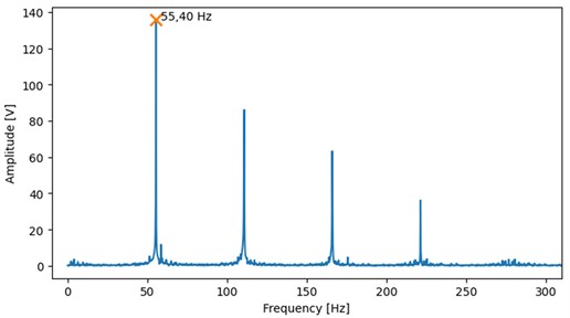
Accurate determination of the shaft’s rotational frequency is fundamental for feature extraction and signal preprocessing. The signal obtained from the tachometer has precisely served this purpose. the peaks of the measured signal in the time domain repeat themselves in synchrony at each shaft rotation. When analysed in the frequency domain shown in Fig. 6, these repetitions appear at a frequency equal to the first dominant peak of the tachometer spectrum, directly reflecting the rotational frequency.
To compute the exact rotational frequency, the method proposed by de Lima et al. [58] and further applied in [55, 56] was adopted. As an illustration, for the tachometer signals measured during operation under an imbalance fault with a severity of 35 g at an input speed of 3,403.776 rpm, the actual measured rotational frequency was calculated to be 55.4 Hz, Fig. 6.
Through the steps described in this chapter, including dataset selection, balancing and normalisation, adjustment of the sampling frequency, and determination of the actual rotational frequency, the dataset has been systematically prepared for further analysis. at this stage, the signals are prepared for preprocessing and feature extraction, the next steps in transforming raw vibration data into compact and informative inputs that are suitable for fault diagnostics using supervised machine learning algorithms.
Fig. 6Measured tachometer signal in the frequency domain
3. Data preprocessing and feature extraction
Once the dataset is prepared, the next step is to process the raw vibration signals to enable their practical application in fault classification. This chapter focuses on the preprocessing procedures and the extraction of features that capture the essential characteristics of machine condition.
3.1. Signal filtering
As previously stated, while creating the dataset, the authors have measured the acceleration of vibration signals over time. According to international standards, the parameter recommended for mechanical vibrations assessment is the root mean square value of vibration velocity, [mm/s] evaluated within the frequency range of 10-1000 Hz [59-61].
For this reason, before using the signals for diagnostic purposes, they must be transformed into the physical quantity of vibration velocity. This is achieved by integrating the acceleration signals along the same axis. However, when the amplitude of the acceleration is measured, the high-frequency components are emphasised, while the low-frequency components are suppressed. Consequently, after integration, a certain distortion of the low-frequency components in the velocity signal is possible, which was not present in the original acceleration signal. To address this issue, a high-pass Butterworth filter is applied before integration. The Butterworth filter is characterised by a smooth response across all frequencies, with a frequency response that monotonically increases or decreases beyond the defined cutoff frequency, depending on whether it is a high-pass or low-pass filter.
In this study, a 6th-order high-pass Butterworth filter was designed with a cutoff frequency set to one-third of the shaft rotational frequency, which removes frequencies lower than this threshold.
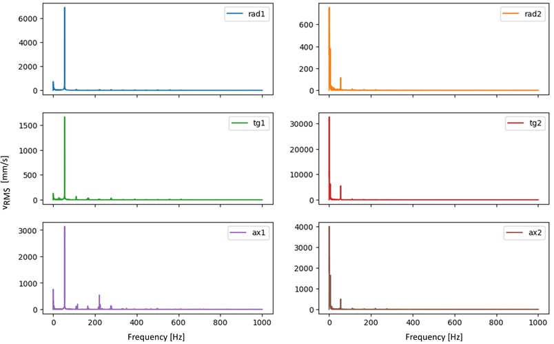
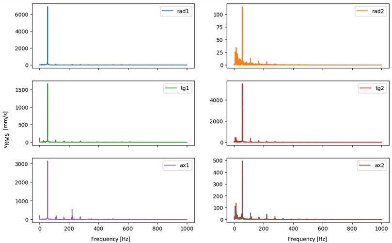
The effectiveness of the designed Butterworth filter is shown in Fig. 7 and 8. The spectrum of the velocity signal obtained by direct integration without using a filter, shows spurious low-frequency peaks unrelated to the actual machine dynamics, Fig. 7 in contrast, the spectrum after applying the high-pass Butterworth filter reveals a clean response where the spurious peaks are eliminated, while the dominant harmonic at the shaft’s rotational frequency of 55.4 Hz remains preserved, Fig. 8. This harmonic corresponds to the characteristic fault frequency for imbalance, which was the operating condition during this test (imbalance of 35 g).
Fig. 7Frequency spectrum of velocity for a signal with an Imbalance of 35 g and rotational frequency of 55.4 Hz before applying the Butterworth Filter (rad1 – radial axis, overhang bearing; rad2 – radial axis, underhang bearing; tg1 – tangential axis, overhang bearing; tg2 – tangential axis, underhang bearing; ax1 – axial axis, overhang bearing; ax2 – axial axis, underhang bearing)
In summary, the designed 6th-order high-pass Butterworth filter effectively eliminates noise and spurious low-frequency components. at the same time, the diagnostic content of the signal is preserved, and the dominant spectral components, which give essential information about the machinery state, remain clearly identifiable. Once the velocity signals are filtered, the root mean square value of vibration velocity () can be calculated within the standardised frequency range of 10-1000 Hz. This parameter will subsequently be used as one of the extracted features, which will be explained in detail in the following section.
Fig. 8Frequency spectrum of velocity for a signal with an Imbalance of 35g and rotational frequency of 55.4 Hz after applying the Butterworth Filter (rad1 – radial axis, overhang bearing; rad2 – radial axis, underhang bearing; tg1 – tangential axis, overhang bearing; tg2 – tangential axis, underhang bearing; ax1 – axial axis, overhang bearing; ax2 – axial axis, underhang bearing)
3.2. Feature extraction
The next step in vibration-based diagnostics using supervised machine learning algorithms is feature extraction, to provide characteristics that quantitatively describe the behaviour of the analysed system. This process transforms complex time domain signals into compact, interpretable numerical indicators that capture the essential characteristics of the analysed machine condition. Extracted features enable the discrimination between healthy and faulty states as well as the differentiation of various fault types. in this section, the set of features extracted from the prepared and processed dataset is presented. It is important to emphasise that the features are extracted from the six signals measured along the three axes and on the two bearing housings. from the velocity signals, the root mean square value () was calculated, as it is one of the most widely used and standardised diagnostic indicators for assessing machine health. From the acceleration signals, spectral parameters were extracted, including the first four harmonics, phase angles, and their sine and cosine values. Furthermore, statistical parameters were obtained from both the time and frequency domains.
The time-domain set includes Root Mean Square (RMS), Standard Deviation (Std), Kurtosis, Skewness, Peak Value, Crest Factor, Impulse Factor, Margin Factor, Shape Factor, and Entropy. The frequency-domain features include Root Mean Square Frequency (RMSF), Frequency Center (FC), and Root Variance Frequency (RVF). Finally, to ensure applicability of the proposed diagnostic framework in varying load conditions, the rotational frequency of the shaft was extracted as a feature. In Nomenclature, the equations for each extracted feature are given.
By extracting these features, the initial seven raw signals in the database, each with 250,000 samples, were transformed into a feature matrix with dimensions 2,147×127, representing 2,147 measurements described by 127 extracted features, Table 4. This compact matrix captures the most informative aspects of the vibration signals, such as amplitude distribution, energy content, frequency composition, and standardised diagnostic parameters, while eliminating the redundancy of raw high-dimensional data. in this way, a suitable input for training and testing supervised machine learning algorithms is obtained.
Table 4Types of extracted features from the dataset
Type | Feature | Number |
– | Rotational frequency of the shaft | 1 |
Statistical parameters of velocity | Root mean square of vibration velocity amplitude () | 6 |
Spectral parameters of acceleration | Harmonics | 24 |
Phase angles | 6 | |
Sine and cosine functions of phase angles | 12 | |
Statistical parameters of acceleration | Time-domain statistical parameters | 60 |
Frequency-domain statistical parameters | 18 | |
Total | 127 |
Through these steps that cover preprocessing and feature extraction, the raw vibration data are transformed into structured and informative feature sets, providing a solid foundation for the application of supervised machine learning algorithms in the subsequent analysis. in the next chapter, this feature matrix will be divided into training and testing subsets. The training set will be used to construct diagnostic models, while the testing set will serve to evaluate and validate their performance. to optimise the feature space and ensure that only the most informative attributes contribute to model training, dimensionality reduction techniques are applied before the use of supervised machine learning algorithms, which is elaborated in the following chapter.
4. Dimensionality reduction and application of supervised machine learning algorithms
Feature matrices can have high dimensionality, which results from the large number of measurements in the dataset and the wide range of features extracted from each measured signal. As the feature space expands, computational costs and training time increase, while irrelevant features may reduce model accuracy. It is essential to emphasise that not all features are equally significant. Some show high significance in diagnosing various machinery states, while others may have a limited impact, and some may even introduce noise into the training process [62]. Moreover, excessively high-dimensional input vectors may increase the risk of overfitting, in which models achieve high accuracy on the training data but fail to generalise effectively to unseen data. To address this issue, various dimensionality reduction techniques are applied to identify and retain only the features with the highest significance in terms of fault diagnostics. As a result, a new feature matrix is generated, which enables training of a model with greater computational efficiency and robustness, while maintaining its representativeness of the machine dynamics. This Chapter proposes and validates a group-wise dimensionality reduction technique that provides complete transparency in assessing the influence of different feature categories and offers a structured framework for reducing dimensionality without compromising the accuracy of classification models. Also, the effectiveness of various supervised machine learning algorithms for fault detection in rotating machinery is tested.
4.1. Sequential selection algorithm (SSA)
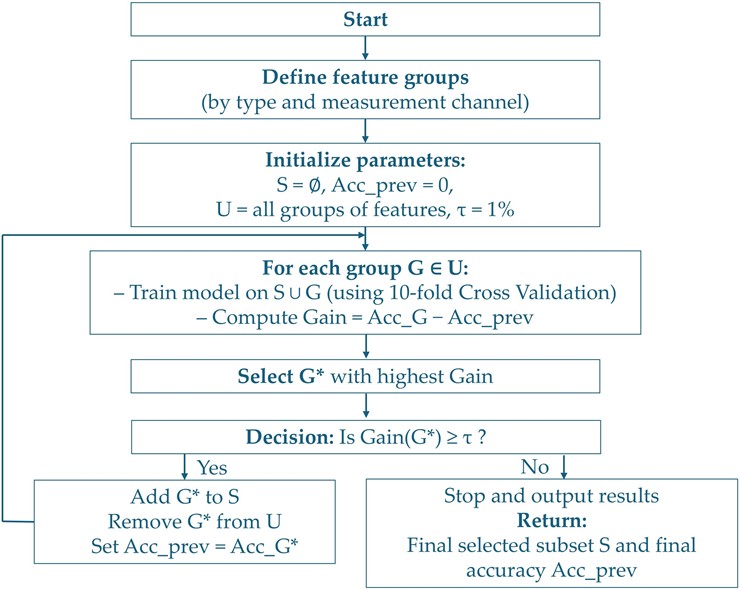
A group-wised dimensionality reduction technique, the Sequential Selection Algorithm (SSA), was proposed in this study. This technique is inspired by classical wrapper-based approaches such as Sequential Forward Selection (SFS) [63] and Recursive Feature Elimination (RFE). SFS starts with an empty set and sequentially adds features, evaluates the selected features, and repeats this process until there is no further improvement in the prediction. RFE starts with a full feature set and eliminates features recursively using weight factors. Unlike these methods, which add or remove individual features, the proposed SSA introduces the concept of group-wise evaluation, where features from same descriptive categories are tested together. More precisely, in this study, features are tested in predefined subsets based on the feature type and measurement along a specific axis and on a specific bearing housing. This approach is particularly important in vibration diagnostics, where extracted features are often correlated and measured across multiple axes and bearing housings. Testing single features in isolation may lead to instability and reduced reliability, as their diagnostic value can be affected by noise measured along a specific axis or variability due to specific sensor placement. By evaluating complete feature groups, SSA enhances both, robustness and replicability of the results, ensuring that diagnostically meaningful relationships are preserved. Furthermore, this group-wise approach significantly improves computational efficiency, as the model is retrained for compact sets of features rather than for each individual feature, reducing the total number of training iterations. Therefore, SSA should not be interpreted as a completely new optimisation principle, but rather as a structured group-wise extension of sequential feature selection specifically designed for vibration-based diagnostics, where physically related features are evaluated collectively instead of individually.
A key principle of the proposed SSA method is the definition of a termination threshold value that ensures both diagnostic relevance and computational efficiency. Specifically, the execution of the algorithm stops once the improvement in classification accuracy obtained by adding a new feature group falls below 1 percentage point (pp). in practice, sequential selection procedures are commonly stopped when adding new variables no longer produces a statistically significant improvement in the objective function [20]. in vibration-based diagnostics, accuracy improvements which are smaller than 1 pp are typically attributed to statistical fluctuations rather than genuine increases in classification ability. Therefore, this criterion prevents the inclusion of redundant or insignificant feature groups, reduces the probability of overfitting and avoids unnecessary model complexity.
The overall procedure of the SSA can be summarized as follows. First, all extracted features are organized into predefined groups according to their type and measurement channel (by the axis and bearing housing from which the signals were measured). Starting from an empty feature set, the algorithm iteratively evaluates each group of features by combining it with the currently selected subset and computing the mean classification accuracy using a 10-fold cross-validation criterium. The gain in accuracy obtained by adding each group is then calculated, and the group which produces the highest gain is incorporated into the subset. This process continues as long as the improvement exceeds the defined threshold. Once no feature group contributes a sufficient improvement in classification accuracy, the algorithm terminates and outputs the final optimized subset of selected features together with the corresponding final model accuracy.
The flowchart in Fig. 9 illustrates the principal steps of the SSA, from feature group definition to defining the termination condition, while the pseudocode in Appendix A2 provides a detailed algorithmic description. Together, these visual and formal representations ensure reproducibility and clarity in the implementation of the proposed technique.
In this Chapter, the methodology used for dimensionality reduction of the input feature matrix using the proposed SSA technique, its validation, and its compatibility with various supervised machine learning algorithms are explained in detail.
4.2. Validation of the sequential selection algorithm (SSA)
The effectiveness of the proposed SSA technique for dimensionality reduction was tested by comparing it with standard methods, such as Principal Component Analysis (PCA), Linear Discriminant Analysis (LDA), and Neighbourhood Component Analysis (NCA). Each of these methods characterises itself with distinct advantages. for instance, PCA transforms the feature space using orthogonal components that capture the maximum variance of the input. LDA projects the input vector or matrix onto a lower-dimensional space that optimises the distinction between separate classes, while NCA assigns a weight factor to all features and retains only those with a value of the weight factor above a previously defined threshold value.
Fig. 9Flowchart of the proposed sequential selection algorithm (SSA)
The resulting inputs from the dimensionality reduction techniques were used to train and evaluate models using supervised machine learning algorithms. More specifically, Support Vector Machines (SVM), k-Nearest Neighbours (k-NN), Random Forests (RF) and Gradient Boosting (XGBoost) were chosen due to their effectiveness in vibration-based fault diagnostics. SVM effectively handles high-dimensional data and nonlinear boundaries using kernel functions. K-NN is characterised as conceptually simple, but benefits substantially from dimensionality reduction because its performance depends directly on distance metrics in feature space. RF, as an ensemble learning method, combines multiple decision trees to achieve robust performance and is particularly effective in handling noisy and imbalanced datasets. XGBoost is a gradient-boosting ensemble method, efficiently captures complex nonlinear relationships through sequential tree optimization. To comprehensively assess the combined effects of dimensionality reduction and supervised learning, each pairing of algorithm and dimensionality reduction technique was systematically trained and tested, creating a complete set of models. An analysis of the contributions of each dimensionality reduction technique and algorithm was conducted to determine the combination which achieved the highest accuracy. In Table 5, the accuracy of testing all models with each pairing of algorithm and dimensionality reduction technique is shown, using a 10-fold cross-validation criterium.
Table 5 presents the results of applying the previously mentioned dimensionality reduction techniques. PCA provided the lowest classification accuracies, indicating that maximal variance by itself does not adequately preserve fault-discriminative information in this context. LDA improved performance by optimising class separability, while NCA further enhanced results by retaining only the features with a weight factor higher than the defined threshold value. the proposed SSA method achieved the highest accuracy using all three algorithms, which validated its effectiveness in identifying feature groups with the highest level of significance in classifying rotating machinery faults.
Table 5Accuracy of testing all models with each pairing of algorithm and dimensionality reduction technique using a 10-fold cross-validation technique
Supervised machine learning algorithm and dimensionality reduction technique | SVM | RF | kNN | XGBoost |
PCA | 62.117±0.62 % | 49.020±0.35 % | 56.709±0.13 % | 50.244±0.47 % |
LDA | 81.405±0.26 % | 74.687±0.97 % | 73.082±0.56 % | 75.434±0.83 % |
NCA | 89.533±0.38 % | 82.234±0.28 % | 87.892±0.24 % | 88.100±0.29 % |
SSA | 95.031 ±0.57 % | 86.594±0.54 % | 90.060±0.46 % | 91.459±0.62 % |
It should be noted that PCA, LDA, and NCA were selected as benchmark methods because they represent some of the most widely used dimensionality-reduction approaches in vibration-based fault diagnosis. Consequently, the comparison presented in Table 5 is intended to evaluate the effectiveness of the proposed SSA relative to established dimensionality-reduction techniques frequently employed in condition monitoring applications.
These outcomes demonstrate that the choice of dimensionality reduction technique plays a critical role in the success of supervised machine learning models for vibration-based diagnostics. The next step in this study is optimisation of diagnostic accuracy and model generalisation by performing hyperparameter tuning of the most effective combinations, particularly SSA paired with each of the classifiers.
4.3. Model optimisation
Hyperparameter tuning is an essential step in training machine learning classifiers because it creates an optimal balance between model complexity, accuracy, and generalisation ability. The optimisation was carried out using grid-search procedures combined with cross-validation, ensuring that the selected parameters obtained robust and reliable results. for the SVM, three hyperparameters were optimised: the kernel function, the value of the regularisation parameter , and the coefficient. The radial basis function (RBF) kernel was selected to enable nonlinear classification across the 10 fault categories. The regularisation parameter was varied across a wide range of values to choose the optimal value, minimising training error and controlling model complexity. The final selected value of C was 481.9212, which ensured a high level of accuracy while preventing overfitting. The final value chosen for the coefficient, which controls the influence of individual data points in the RBF kernel, was 0.0018. for the RF classifier, the primary hyperparameter considered was the number of decision trees (estimators). While the default value in scikit-learn is 100, experiments tested values up to 2000. The results showed that classification accuracy increased steadily as the number of trees increased and reached a stable maximum at approximately 800 estimators, beyond which no significant improvement in accuracy was achieved. Therefore, the optimal configuration was set at 800 trees. Other parameters, such as maximum tree depth, minimum samples per split, and minimum samples per leaf, were found to have limited impact on performance and were thus retained at their default values in the scikit-learn library in Python. for the k-NN algorithm, optimisation was performed on two key parameters: the number of neighbours k and the distance metric. Euclidean distance was chosen as the distance metric, and the number of neighbours was varied from 1 to 30, with an accuracy peak at a value of 11. for the XGBoost classifier, optimisation focused on the parameters that control the depth, learning behaviour, and number of boosted trees. The final selected configuration consisted of a learning rate of 0.1, a maximum depth of 2, and 250 estimators. The shallow tree depth prevented overfitting, while the chosen learning rate ensured stable convergence, and the number of trees provided sufficient model capacity to achieve high classification accuracy.
The accuracy of the optimised models is clearly higher than the classification accuracy compared to their default configurations. After hyperparameter tuning, Table 6, SVM achieved the highest accuracy of 97.060 %, followed by k-NN with 92.371 %, RF with 91.722 %, and XGBoost with 93.334 %. These results confirm the importance of parameter optimisation in enhancing diagnostic performance and highlight the strong synergy between SSA and SVM for vibration-based fault classification.
Table 6Accuracy of testing SSA with each algorithm after hyperparameter tuning using a 10-fold cross-validation technique
Supervised machine learning algorithm | SVM | RF | kNN | XGBoost |
Accuracy after hyperparameter tuning | 97.060±0.59 % | 91.722±0.64 % | 92.371±0.25 % | 93.334±0.46 % |
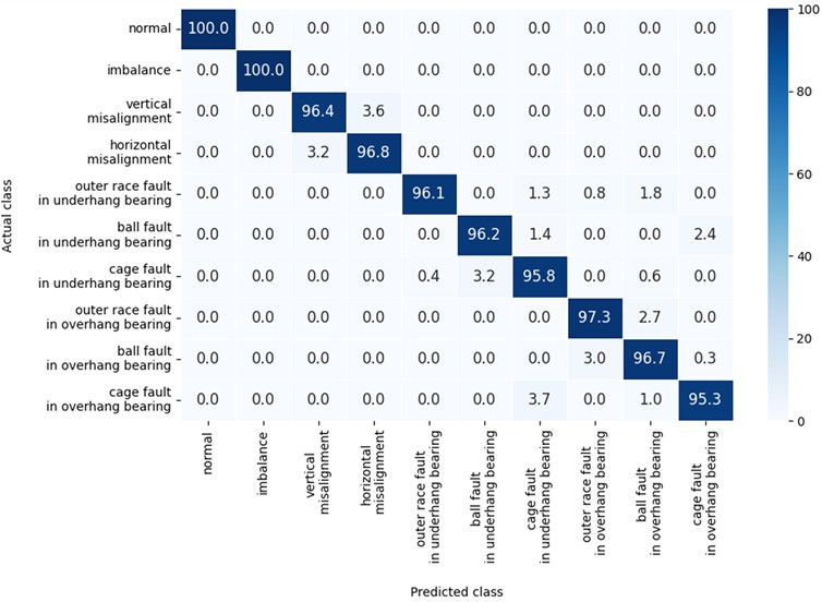
As previously mentioned, vibration datasets often exhibit class imbalance, which may lead to poor accuracy on underrepresented fault classes. in this paper, the dataset balancing methodology described in Section 2.2 was applied to reduce bias toward dominant classes and ensure a more equitable distribution of samples. Moreover, evaluating model performance solely through overall accuracy may obscure weaknesses in detecting minority classes. for this reason, a confusion matrix is also generated to examine per-class recognition accuracy and assess diagnostic robustness across all ten fault categories. Fig. 10 presents the confusion matrix obtained for the classifier with the highest performance, which combines the proposed SSA dimensionality reduction method with the SVM algorithm. After hyperparameter optimisation, this combination achieved an overall classification accuracy of 97.060 % using 10-fold cross-validation.
It can be seen from the confusion matrix that highest values are present in the main diagonal, which confirms that most samples were correctly classified in the actual fault categories. High accuracy above 95 % is observed across all fault types, highlighting the robustness of the proposed diagnostic framework. Minor error can be seen only between closely related classes, e.g., vertical vs. horizontal misalignment, and in distinguishing certain bearing fault classes, which is expected due to their similarity in vibration signatures. These results validate SSA-SVM as the most effective approach, ensuring both high accuracy and strong generalization for vibration-based fault classification.
Although the obtained results demonstrate the effectiveness of the proposed SSA-SVM combination, the SSA methodology shares conceptual similarities with the classical Sequential Forward Selection (SFS) technique. Therefore, an additional comparative analysis was conducted to evaluate the influence of the proposed group-wise feature selection strategy.
4.4. Comparison of SSA with sequential forward selection
Since the proposed SSA is conceptually related to Sequential Forward Selection (SFS), an additional comparison was conducted to evaluate the effect of the proposed group-wise selection strategy. Classical SFS was applied to the same feature matrix and evaluated using the same optimized SVM classifier. The final performance of both methods was evaluated using 10-fold cross-validation. Table 7 summarizes the obtained results. It should be noted that the objective of this comparison is not to demonstrate that SSA introduces a fundamentally new optimisation principle, but rather to evaluate the effectiveness of the proposed group-wise selection strategy in comparison with conventional feature-level SFS.
The results indicate that the proposed SSA achieves a classification accuracy comparable to that of conventional SFS. The difference in classification accuracy between the two methods is only 0.07 percentage points, while SSA selects a slightly smaller feature subset (29 compared to 33 features). Furthermore, SSA requires substantially lower computational effort during feature selection, reducing the feature-selection time from 474.56 s to 27.40 s, corresponding to a 94.2 % reduction in computational effort during feature selection. in addition, the group-wise selection strategy preserves physically meaningful relationships between vibration features originating from the same measurement channel, which improves interpretability and facilitates the analysis of feature importance from a vibration-diagnostic perspective.
Table 7Comparison of the proposed sequential selection algorithm (SSA) and classical sequential forward selection (SFS)
Method | Selection strategy | Selected features | Accuracy [%] | Feature selection time [s] |
SFS | Individual feature selection | 33 | 97.130±1.216 | 474.56 |
Proposed SSA | Group-wise feature selection | 29 | 97.060±0.590 | 27.40 |
4.5. Level of importance of feature groups
As priorly mentioned, in conducting the SSA method, the accuracy of the model based on SVM is tested sequentially using various groups of features, categorised by their type and nature. in this part, the pipeline of the proposed SSA method will be explained in detail. From Table 7, it is evident that the classifier's accuracy varies significantly depending on the type of input features. The table also reports the number of input features included in each group. It is essential to emphasise that the rotational frequency was consistently included in all groups, since this parameter directly influences the values of the remaining features and thus represents a fundamental input for reliable fault diagnosis.
Fig. 10Confusion matrix using SSA and SVM after hyperparameter tuning
According to the results presented in Table 8, the accuracy obtained when using only the statistical features (85 in total) as inputs for training the SVM-based classifier was nearly identical (97.071 %) to the accuracy achieved when all 127 extracted features were employed (97.074 %), with a difference of less than 1 %. To further investigate the potential for dimensionality reduction of the SSA method, the performance was evaluated using features extracted from signals recorded along each of the three axes and at both bearing locations, Table 9. The results demonstrate that features derived from the radial axis of overhang and underhang bearings provide an accuracy of 97.060 % which is very close to that obtained when using features from all axes (97.071 %), again with a difference of less than 1 %.
In other words, training the SVM classifier with only 29 statistical features, 14 from the radial axis of each bearing and the rotational frequency, resulted in an accuracy of 97.060 % using 10-fold cross-validation. These results indicate that a reduced feature set, which contains the features with the highest level of significance, can achieve the same diagnostic performance as the complete set while notably reducing the dimensionality of the input space. The initial results in Table 6 present the accuracy of the optimised models, which were trained using only these 29 input features.
The obtained results confirm that a systematically designed dimensionality reduction method can result in a feature matrix suitable for training a model that achieves high accuracy in the testing phase, while ensuring greater generalizability and efficiency. Additionally, the proposed SSA method enables the clear identification of feature sets that show the highest significance in improving classification accuracy by sequentially testing the influence of feature groups, thereby enhancing the transparency and interpretability of the results. in this case, the combination of SSA as a method for dimensionality reduction and SVM as a supervised machine learning algorithm produces a model with high accuracy, robustness and reliability, while reducing the risk of overfitting.
Table 8Accuracy of the model based on SVM by sequentially using different groups of features based on their type when applying SSA
Groups of features | Number of features | Accuracy |
Phase angles and | 7 | 77.319±0.69 % |
Sine and cosine functions of phase angles and | 13 | 77.523±0.53 % |
Harmonics and | 25 | 80.458±0.39 % |
Harmonics, Sine and cosine functions of phase angles and | 37 | 91.369±0.52 % |
Root mean square of vibration velocity amplitude () and | 7 | 71.273±0.70 % |
Statistical parameters of velocity and acceleration in the time-domain and | 67 | 93.337±0.41 % |
Statistical parameters of acceleration in the frequency-domain and | 19 | 93.589±0.63 % |
All Statistical parameters and | 85 | 97.071±0.42 % |
All Features | 127 | 97.074±0.29 % |
Table 9Accuracy of the model based on SVM by sequentially using signals measured along different axes and on different bearing housings when applying SSA
Axis | Overhang bearing | Underhang bearing | Overhang and underhang bearing |
Axial | 78.514±0.85 % | 78.423±0.44 % | 84.217±0.47 % |
Radial | 89.992±0.54 % | 92.934±0.12 % | 97.060±0.59 % |
Tangential | 88.296±0.31 % | 91.579±0.88 % | 92.721±0.51 % |
All axes | 95.984±0.77 % | 96.922±0.66 % | 97.071±0.42 % |
The dominance of the radial-axis features can be explained by the physical nature of the faults included in the analysed dataset. Imbalance generates a centrifugal force proportional to the rotating mass and the square of the rotational speed, which acts predominantly in the radial direction. Consequently, radial vibration components contain the strongest signatures associated with imbalance faults.
Similarly, rolling bearing defects produce repeated impact forces at the rolling element-raceway contacts. These impacts are transmitted primarily through the bearing housing in the radial direction, resulting in increased radial vibration amplitudes and more pronounced statistical indicators. Therefore, radial-axis measurements are expected to contain a higher concentration of diagnostically relevant information for bearing fault classification.
In contrast, axial vibration components are typically more sensitive to axial loading conditions and certain forms of shaft misalignment. Although axial vibration components are commonly associated with shaft misalignment, the analysed dataset contains a larger number of fault categories dominated by radial vibration responses, particularly imbalance and rolling bearing defects. Consequently, radial features provide greater overall discriminative capability for the complete multi-class classification problem. Nevertheless, axial features still contribute useful diagnostic information. The obtained results indicate that they are less effective when considered independently for distinguishing the complete set of analysed fault categories. A similar observation applies to tangential measurements, which contain fault-related information but generally exhibit lower sensitivity to the dominant dynamic effects generated by imbalance and bearing defects.
The obtained results therefore suggest that, for the analysed dataset, the most discriminative information is concentrated in the radial measurements acquired on both bearing housings. This observation is consistent with vibration diagnostic theory, according to which radial responses are often the most sensitive indicators of imbalance and rolling bearing faults.
Furthermore, although SSA performs data-driven selection of feature groups, the retained features remain consistent with established mechanical vibration theory. The prominence of lower-order harmonics is consistent with the characteristic 1× rotational component associated with imbalance and the 2× rotational components frequently observed in misalignment conditions. Likewise, time-domain statistical features such as RMS, kurtosis, and crest factors are recognised descriptors of localized impacts produced by rolling bearing defects. The fact that SSA prioritises these physically meaningful feature groups supports the interpretability of the reduced feature space and provides a physically grounded explanation of the obtained classification results.
5. Estimating computational efficiency of the framework
A complete assessment of a proposed framework for vibration-based diagnostics requires not only evaluating its classification accuracy but also analysing its computational efficiency. Therefore, this chapter presents two complementary analyses aimed at quantifying the computational behaviour of the proposed pipeline.
First, a sensitivity analysis of the proposed method for reducing the sampling frequency is performed to evaluate its effects on the diagnostic performance and the computational costs. This analysis provides insight into the extent to which the vibration signals can be downsampled without compromising the discriminative information required for reliable fault detection.
Second, the computational efficiency of the Sequential Selection Algorithm (SSA) is examined by determining the computational time for training and testing the supervised machine learning algorithms with and without applying SSA. Since SSA is a central component of the proposed methodology, understanding its benefits in terms of reducing computational time is essential for evaluating its suitability for practical applications.
Overall, these analyses offer a comprehensive overview of the efficiency and scalability of the proposed framework, complementing the accuracy results presented in the previous chapter.
5.1. Sensitivity analysis of the downsampling method
To evaluate the robustness of the proposed downsampling method and quantify the potential loss of diagnostic information, a sensitivity analysis is performed across a range of downsampling ratios. Starting from the original 50 kHz measurements, the vibration signals are downsampled using ratios between 5 and 50, corresponding to sampling frequencies from 10 kHz to 1 kHz. for each value of the downsampling ratio, the same preprocessing procedure, which includes applying an anti-aliasing filter, amplitude normalisation, dataset balancing and feature extraction, is carried out prior to model training. The combination of a SVM algorithm and the SSA method is used, and the 10-fold cross-validation criterium is applied. Table 10 summarises the obtained accuracy of the diagnostics model, and the computation time required for feature extraction of all 127 features.
The results show that the proposed framework is highly robust to moderate reductions in sampling frequency. for ratios between 5 and 12, corresponding to 10-4.17 kHz, the accuracy remains consistently above 96.7 %, with variations below 1 pp. This confirms that the spectral content which carries significant diagnostic information is preserved even after downsampling. On the other hand, the computational time for feature extraction decreases rapidly with increasing the downsampling ratio. The computation time for feature extraction drops from approximately 73 minutes at a downsampling ratio of 5, to less than 17 minutes at a ratio of 10 and converges to a stable value for ratios above 20.
Table 10Sensitivity analysis of the proposed downsampling method: computation time for feature extraction and achieved accuracy
Ratio | Downsampled (kHz) | Calculation time for feature extraction | SVM+SSA accuracy (%) |
5 | 10.00 | 72 min 57.6 s | 97.319±0.59 |
6 | 8.33 | 34 min 4.0 s | 97.312±0.63 |
7 | 7.14 | 21 min 34.50 s | 97.304 + 0.67 |
8 | 6.25 | 20 min 38.70 s | 97.111±0.70 |
9 | 5.56 | 19 min 18.16 s | 97.081±0.62 |
10 | 5.00 | 17 min 23.40 s | 97.060±0.59 |
11 | 4.55 | 16 min 53.90 s | 97.004±0.78 |
12 | 4.17 | 16 min 48.17 s | 96.765±0.80 |
13 | 3.85 | 16 min 45.12 s | 96.622±0.52 |
14 | 3.57 | 16 min 37.14 s | 96.491±0.66 |
15 | 3.33 | 16 min 29.30 s | 96.358±0.65 |
20 | 2.50 | 15 min 58.70 s | 95.912±0.71 |
30 | 1.67 | 15 min 48.20 s | 95.337±0.83 |
40 | 1.25 | 15 min 38.73 s | 94.981± 0.54 |
50 | 1.00 | 15 min 32.50 s | 94.641±0.64 |
The sensitivity analysis demonstrates that the proposed downsampling method is both efficient and reliable. Substantial reductions in computational cost can be achieved with only minor impact on diagnostic performance, confirming the practicality of the proposed framework for real-time or resource-constrained industrial applications.
Considering the obtained results and the recommendations of international standards, a downsampling ratio of 10 is selected as the most appropriate configuration. Firstly, from the sensitivity analysis it can be seen that this value provides a robust compromise between diagnostic fidelity and computational efficiency. The sensitivity analysis shows that this ratio offers a stable compromise between diagnostic fidelity and computational efficiency, maintaining high classification accuracy while significantly reducing the time for feature extraction. At the same time, the resulting effective sampling rate of 5 kHz remains fully aligned with guidelines for magnetic sensor mounting, ensuring that all diagnostically relevant frequency components areretained.
5.2. Computational efficiency of the sequential selection algorithm (SSA)
A key motivation behind the proposed Sequential Selection Algorithm (SSA) is not only to improve diagnostic accuracy but also to reduce computational costs, which is an essential requirement for practical industrial applications. To quantify the efficiency gains achieved by SSA, the time required for training and testing each evaluated model is compared before and after applying the SSA method for dimensionality reduction.
Table 11 summarises the results for the time required for training and testing of SVM, Random Forest, k-NN, and XGBoost using the full set of 127 features and the reduced feature set generated by SSA. Across all models, a consistent reduction in execution time is observed when SSA is applied. Although, the magnitude of improvement varies depending on the computational characteristics of each algorithm and its nature, the trend is uniform: applying the SSA leadsto shorter computational time.
Beyond computational time reduction, it is important to evaluate the economic efficiency of the proposed diagnostic framework. for this purpose, an Economic Efficiency Factor (EEF) is introduced, Eq. (6):
where is the required time for training and testing using the full set of 127 features and is the required time for training and testing using the reduced feature set obtained with SSA. The EEF expresses the percentage reduction in computational cost, and reflects potential savings in industrial deployments, particularly in systems with limited processing capacity or high-frequency monitoring requirements.
Table 11Required time for training and testing each classifier before and after applying SSA
Model | Time for training and testing using full feature set | Time for training and testing after applying SSA | EEF [%] |
SVM | 93.51 s | 53.72 s | 42.55 |
RF | 74.37 s | 48.12 s | 35.29 |
kNN | 28.84 s | 15.92 s | 44.79 |
XGBoost | 3331.69 s | 825.45 s | 75.22 |
These results show that the proposed SSA method provides substantial computational and economic benefits. The most apparent improvement is observed for XGBoost, where total execution time decreases from 3331.69 s to 825.45 s which is a nearly four-fold speed-up corresponding to a 75 % reduction in computational cost. SVM, one of the most widely used algorithms in vibration-based diagnostics, also benefits significantly, with training and testing time reduced from 93.51 s to 53.72 s (EEF = 42.6 %). Similar improvements are seen in k-NN (EEF = 44.8 %), where dimensionality reduction directly decreases distance computations, and in Random Forest (EEF = 35.3 %), where fewer feature splits are evaluated during tree construction.
It should be noted that the execution times reported in Table 11 correspond exclusively to the training and testing stages of the evaluated classifiers. Since the proposed SSA method introduces an additional feature-selection stage, its computational overhead must also be considered when assessing the overall computational cost of the framework.
For the analysed dataset, the execution time required for the SSA feature-selection procedure was 27.40 s (Table 7). Consequently, the total execution time of the SSA-SVM framework, including both feature selection and classifier training/testing, was 81.12 s. Although the inclusion of the feature-selection stage reduces the net computational gain compared with considering classifier execution time alone, the overall execution time remains lower than that required for training and testing the SVM using the full feature set (93.51 s). It should also be emphasised that feature selection represents a one-time offline optimisation step, whereas classifier training and testing may be repeated multiple times during model development and deployment. Furthermore, the computational cost of the proposed SSA remains substantially lower than that required by classical Sequential Forward Selection (474.56 s), while simultaneously providing a reduced feature space and improved interpretability.
Overall, the results confirm that SSA substantially reduces the dimensionality of the feature space while maintaining the diagnostic accuracy presented in Section 4. The computational benefits are particularly evident for computationally demanding classifiers such as SVM and XGBoost, where the reduction in training and testing time is substantially greater than the additional cost associated with feature selection. for less computationally intensive classifiers, such as k-NN and Random Forest, the one-time feature-selection overhead may partially offset the reduction in classifier execution time. Nevertheless, SSA provides a compact and physically interpretable feature subset, which facilitates model development and reduces the complexity of subsequent diagnostic analyses. These advantages make SSA a practical dimensionality-reduction approach for vibration-based diagnostic systems, particularly in applications involving high-dimensional feature spaces and computationally demanding machine-learning models.
6. Conclusions, limitations and future work
The following subsections present the main conclusions of this study, together with a discussion of its current limitations and future research directions.
6.1. Conclusions
This study presents a comprehensive framework for fault diagnostics of rotating machinery that integrates dataset preparation, signal preprocessing, feature extraction, dimensionality reduction, and training and testing of supervised machine learning algorithms. Dataset preparation, preprocessing and feature extraction transform raw vibration signals into informative, structured feature matrices, ensuring data quality and compliance with international standards. A diverse set of time-domain, frequency-domain, and spectral parameters, capturing the statistical, harmonic, and phase-related characteristics of machine behaviour are extracted.
To optimise high-dimensional feature spaces and allow transparency in identifying features with the highest level of importance in recognising machinery faults, a group-wise dimensionality reduction technique, Sequential Selection Algorithm (SSA), was proposed. Its performance was compared to that of three commonly used dimensional reduction techniques: PCA, LDA, and NCA. The results obtained under the conditions of this study indicate that SSA offers favourable performance relative to the other techniques and may be a useful tool when designing automated diagnostic systems for rotating machinery. Also, the effectiveness of three supervised machine learning algorithms, SVM, k-NN, RF, and XGBoost for vibration-based fault classification was confirmed. The combination of SSA dimensionality reduction technique and SVM classifier achieved an accuracy of 97.06 % using 10-fold cross-validation technique, with only 29 input features.
Overall, the findings suggest that careful integration of advanced data preparation, feature extraction, dimensionality reduction, and machine learning methods can contribute to the development of reliable and efficient vibration-based diagnostic frameworks. Moreover, the results show that increasing the number of features does not necessarily improve diagnostic accuracy and performance. Also, carefully designed dimensionality reduction strategies can eliminate redundancy, reduce the risk of overfitting, and enhance model interpretability, while maintaining or even improving its accuracy.
In addition to diagnostic performance, this study also evaluated the computational and economic efficiency of the proposed framework. The results presented in Chapter 5 indicate that the proposed SSA technique substantially reduces the required time for training and testing across all evaluated classifiers, yielding efficiency gains of up to 75 % without compromising accuracy. These improvements suggest that the framework may be suitable for deployment in resource-constrained or real-time industrial environments, where computational cost is a critical consideration.
6.2. Limitations and future work
Although the Machinery Fault Database is one of the largest and most complete open-access datasets for vibration-based fault diagnostics, several limitations must be acknowledged. All measurements were acquired on a single laboratory test rig which operated under controlled conditions and in the presence of simulated faults. As a result, the variability in working conditions, mounting conditions, background noise, and unexpected external impacts is lower than in industrial environments, where machines operate under changing regimes and are exposed to various environmental disturbances. The dataset also covers only a subset of common faults (imbalance, misalignment, and defects in rolling bearings) and does not include combinations of simultaneous faults. in addition, the measurements were performed using a specific bearing type and machinery simulator, which may limit the direct application of the trained models to machines with different geometry or dynamic properties.
It must also be emphasized that real industrial machinery typically exhibits non-stationary behaviour, speed variability, transient conditions, and load fluctuations. in this study, the diagnostic framework was evaluated using measurements with a tachometer-based rotational speed signal and therefore assumes the availability of accurate speed information. Tacholess speed estimation, adaptive order tracking, and frequency-invariant feature extraction, which are essential under highly variable operating conditions, were not incorporated in the present work and remain important challenges.
These limitations highlight the need to validate the proposed framework on industrial data before fully generalizing it. Accordingly, the findings presented here should be interpreted in the context of the controlled laboratory conditions of the Machinery Fault Database, which do not fully capture the variability and complexity of industrial operating environments.
Finally, this study focuses on the application of supervised machine learning algorithms combined with structured feature engineering and a transparent dimensionality-reduction method. Although recent advances in deep learning, including convolutional neural networks, transformer-based architectures, and graph-based learning methods, have demonstrated promising results in machinery fault diagnosis, a direct comparison with such approaches was beyond the scope of the present study. Future research should therefore include a systematic evaluation of the proposed framework against modern deep-learning architectures using the same datasets and validation procedures.
References
-
V. Wonk, Machinery Vibration-Measurement and Analysis. New York, NY, USA: McGraw-Hill, 1991.
-
A. K. S. Jardine, D. Lin, and D. Banjevic, “A review on machinery diagnostics and prognostics implementing condition-based maintenance,” Mechanical Systems and Signal Processing, Vol. 20, No. 7, pp. 1483–1510, Nov. 2005, https://doi.org/10.1016/j.ymssp.2005.09.012
-
J. Lee, F. Wu, W. Zhao, M. Ghaffari, L. Liao, and D. Siegel, “Prognostics and health management design for rotary machinery systems-reviews, methodology and applications,” Mechanical Systems and Signal Processing, Vol. 42, No. 1-2, pp. 314–334, Aug. 2013, https://doi.org/10.1016/j.ymssp.2013.06.004
-
R. B. Randall, Vibration-Based Condition Monitoring: Industrial, Aerospace and Automotive Applications. Chichester, U.K.: Wiley, 2011, https://doi.org/10.1002/9780470977668
-
A. Rai and S. H. Upadhyay, “A review on signal processing techniques in rotating machinery fault diagnosis,” Mechanical Systems and Signal Processing, Vol. 25, pp. 123–146, 2016.
-
M. Elforjani and D. Mba, “Condition monitoring of slow-speed rolling element bearings using acoustic emission technique,” Mechanical Systems and Signal Processing, Vol. 23, pp. 115–124, 2009.
-
D. Yang, X. Wang, and C. Wu, “A review of vibration-based signal processing techniques for rotating machinery fault diagnosis,” Applied Sciences, Vol. 11, p. 11073, 2021.
-
S. Yin, X. Li, H. Gao, and O. Kaynak, “Data-based techniques focused on modern industry: an overview,” IEEE Transactions on Industrial Electronics, Vol. 62, No. 1, pp. 657–667, Feb. 2014, https://doi.org/10.1109/tie.2014.2308133
-
P. W. Tse, Y. H. Peng, and R. Yam, “Wavelet analysis and envelope detection for rolling element bearing fault diagnosis-their effectiveness and flexibilities,” Journal of Vibration and Acoustics, Vol. 123, No. 3, pp. 303–310, Jul. 2001, https://doi.org/10.1115/1.1379745
-
J. Lee, H.-A. Kao, and S. Yang, “Service innovation and smart analytics for industry 4.0 and big data environment,” Procedia CIRP, Vol. 16, pp. 3–8, Jul. 2014, https://doi.org/10.1016/j.procir.2014.02.001
-
R. Walker, S. Perinpanayagam, and I. K. Jennions, “Rotordynamic faults: recent advances in diagnosis and prognosis,” International Journal of Rotating Machinery, Vol. 2013, pp. 1–12, Feb. 2013, https://doi.org/10.1155/2013/856865
-
A. H. Samsudin, “Predictive modelling of hybrid composite laminates buckling behaviour using finite element analysis, refined response surface methodology and artificial neural network models with different data sizes,” Journal of Mechanical Engineering, Vol. 23, No. 1, pp. 179–211, Jan. 2026, https://doi.org/10.24191/jmeche.v23i1.9426
-
A. Al-Obaidi et al., “Finite element and artificial neural network-based buckling load analysis of cylindrical structures: impact of training data proportions,” in Proceedings of the 2025 IEEE 2nd International Conference on Computing, Artificial Intelligence and Intelligent Systems (I2CACIS), pp. 1–6, 2025, https://doi.org/10.1109/i2cacis65476.2025.11101549
-
O. Das, D. Bagci Das, and D. Birant, “Machine learning for fault analysis in rotating machinery: a comprehensive review,” Heliyon, Vol. 9, No. 6, p. e17584, Jun. 2023, https://doi.org/10.1016/j.heliyon.2023.e17584
-
D. Latil, R. Houé Ngouna, K. Medjaher, and S. Lhuisset, “Vibration-based data-driven fault diagnosis of rotating machines operating under varying working conditions,” International Journal of Prognostics and Health Management, Vol. 16, No. 2, Jul. 2025, https://doi.org/10.36001/ijphm.2025.v16i2.4208
-
Y. Lei, N. Li, L. Guo, N. Li, T. Yan, and J. Lin, “Machinery health prognostics: a systematic review from data acquisition to RUL prediction,” Mechanical Systems and Signal Processing, Vol. 104, pp. 799–834, Dec. 2017, https://doi.org/10.1016/j.ymssp.2017.11.016
-
A. Malhi, R. Yan, and R. X. Gao, “Prognosis of defect propagation based on recurrent neural networks,” IEEE Transactions on Instrumentation and Measurement, Vol. 60, No. 3, pp. 703–711, Feb. 2011, https://doi.org/10.1109/tim.2010.2078296
-
A. Widodo and B.-S. Yang, “Support vector machine in machine condition monitoring and fault diagnosis,” Mechanical Systems and Signal Processing, Vol. 21, No. 6, pp. 2560–2574, Jan. 2007, https://doi.org/10.1016/j.ymssp.2006.12.007
-
H. Liu and H. Motoda, Feature Selection for Knowledge Discovery and Data Mining. Boston, MA: Springer US, 2011, https://doi.org/10.1007/978-1-4615-5689-3
-
I. Guyon and A. Elisseeff, “An introduction to variable and feature selection,” Journal of Machine Learning Research, Vol. 3, pp. 1157–1182, 2003.
-
H. Peng, F. Long, and C. Ding, “Feature selection based on mutual information: criteria of max-dependency, max-relevance, and min-redundancy,” IEEE Transactions on Pattern Analysis and Machine Intelligence, Vol. 27, No. 8, pp. 1226–1238, 2005, https://doi.org/10.1109/tpami.2005.159
-
G. Brito, J. R. A. Amazonas, and J. P. Papa, “A comparative study of dimensionality reduction techniques for feature-based anomaly detection in bearings,” Informatics, Vol. 8, No. 85, 2021.
-
D. Neupane, M. R. Bouadjenek, R. Dazeley, and S. Aryal, “Data-driven machinery fault diagnosis: a comprehensive review,” Neurocomputing, Vol. 627, p. 129588, Feb. 2025, https://doi.org/10.1016/j.neucom.2025.129588
-
M. Tiboni, C. Remino, R. Bussola, and C. Amici, “A review on vibration-based condition monitoring of rotating machinery,” Applied Sciences, Vol. 12, No. 3, p. 972, Jan. 2022, https://doi.org/10.3390/app12030972
-
J. Pelayo-González, C. Rubio-Anaya, and F. A. Ortiz-Luna, “Bearing fault diagnosis with envelope analysis and machine learning approaches using CWRU dataset,” Engineering Proceedings, Vol. 46, No. 23, 2025.
-
H. Zhang, Y. Chen, and X. Li, “Intelligent fault diagnosis of rotating machinery using improved SVM with feature dimensionality reduction,” Applied Sciences, Vol. 10, p. 10217, 2020.
-
Z. Wang, J. Cao, Y. Zhang, and Z. Chen, “Fault diagnosis method for rolling bearings based on VMD, RCMWPE, t-SNE, and WOA-SVM,” Sensors, Vol. 25, 2025, https://doi.org/10.20855/ijav.2026.31.12130
-
M. T. Singh, “Graph-based fault diagnosis for rotating machinery: adaptive segmentation and structural feature integration,” Results in Engineering, Vol. 27, p. 106566, Aug. 2025, https://doi.org/10.1016/j.rineng.2025.106566
-
W. Shen, M. Xiao, Z. Wang, and X. Song, “Rolling bearing fault diagnosis based on support vector machine optimized by improved grey wolf algorithm,” Sensors, Vol. 23, No. 14, p. 6645, Jul. 2023, https://doi.org/10.3390/s23146645
-
K. Adamsab, “Machine learning algorithms for rotating machinery bearing fault diagnostics,” Materials Today: Proceedings, Vol. 44, pp. 4931–4933, Jan. 2021, https://doi.org/10.1016/j.matpr.2020.12.050
-
A. Dineva, A. Mosavi, M. Gyimesi, I. Vajda, N. Nabipour, and T. Rabczuk, “Fault diagnosis of rotating electrical machines using multi-label classification,” Applied Sciences, Vol. 9, No. 23, p. 5086, 2019, https://doi.org/10.3390/app9235086
-
H. Zhou, Y. Chen, and J. Yang, “Fault diagnosis of shaft imbalance and angular misalignment in rotating machinery using SVM and decision tree classifiers,” Mechanical Systems and Signal Processing, Vol. 138, p. 2019, 2020.
-
Y. Cao, L. Xu, and B. Wang, “Feature selection and classification of imbalance and misalignment faults in rotating machinery,” Measurement, Vol. 174, 2021.
-
N. Rezazadeh, A. de Luca, and D. Perfetto, “Unbalanced, cracked, and misaligned rotating machines: a comparison between classification procedures throughout the steady-state operation,” Journal of the Brazilian Society of Mechanical Sciences and Engineering, Vol. 44, No. 10, Sep. 2022, https://doi.org/10.1007/s40430-022-03750-1
-
B. T. Atmaja, H. Ihsannur, Suyanto, and D. Arifianto, “Lab-scale vibration analysis dataset and baseline methods for machinery fault diagnosis with machine learning,” Journal of Vibration Engineering and Technologies, Vol. 12, No. 2, pp. 1991–2001, 2023, https://doi.org/10.1007/s42417-023-00959-9
-
H. H. Huynh and C.-H. Min, “Rotating machinery fault detection using support vector machine via feature ranking,” Algorithms, Vol. 17, No. 10, p. 441, Oct. 2024, https://doi.org/10.3390/a17100441
-
J. Li, W. Sun, and M. Zhao, “A fault diagnosis method for rotating machinery under variable working conditions based on domain adaptation and SVM,” Sensors, Vol. 21, 2021.
-
H. Patel and S. H. Upadhyay, “Fault diagnosis of rotating machinery using vibration signal features and machine learning classifiers,” Journal of Vibroengineering, Vol. 23, pp. 282–296, 2021.
-
A. K. Ovacıklı, M. Yagcioglu, S. Demircioglu, T. Kocatekin, and S. Birtane, “Supervised learning-based fault classification in industrial rotating equipment using multi-sensor data,” Applied Sciences, Vol. 15, No. 13, p. 7580, 2025, https://doi.org/10.3390/app15137580
-
H. Nyquist, “Certain topics in telegraph transmission theory,” Transactions of the American Institute of Electrical Engineers, Vol. 47, No. 2, pp. 617–644, Jun. 2009, https://doi.org/10.1109/t-aiee.1928.5055024
-
C. E. Shannon, “Communication in the presence of noise,” Proceedings of the IRE, Vol. 37, No. 1, pp. 10–21, Jun. 2007, https://doi.org/10.1109/jrproc.1949.232969
-
J. Luo, L. Zhu, Q. Li, and M. Chen, “Imbalanced fault diagnosis of rotating machinery using WGAN-GP,” Processes, Vol. 9, 2021.
-
M. Jalayer, A. Kaboli, C. Orsenigo, and C. Vercellis, “Fault detection and diagnosis with imbalanced and noisy data: a hybrid framework for rotating machinery,” Machines, Vol. 10, No. 4, p. 237, 2022, https://doi.org/10.3390/machines10040237
-
W. Zhang, G. Peng, C. Li, Y. Chen, and Z. Zhang, “A new deep learning model for fault diagnosis with good anti-noise and domain adaptation ability on raw vibration signals,” Sensors, Vol. 17, No. 2, p. 425, 2017, https://doi.org/10.3390/s17020425
-
T. Ince, S. Kiranyaz, L. Eren, M. Askar, and M. Gabbouj, “Real-time motor fault detection by 1-D convolutional neural networks,” IEEE Transactions on Industrial Electronics, Vol. 63, No. 11, pp. 7067–7075, 2016, https://doi.org/10.1109/tie.2016.2582729
-
R. Zhao, R. Yan, Z. Chen, K. Mao, P. Wang, and R. X. Gao, “Deep learning and its applications to machine health monitoring: a survey,” ISA Transactions, Vol. 64, pp. 851–864, 2019, https://doi.org/10.48550/arxiv.1612.07640
-
Z. Chen, K. Gryllias, and W. Li, “Mechanical fault diagnosis using convolutional neural networks and transfer learning,” IEEE Transactions on Industrial Electronics, Vol. 68, No. 3, pp. 2526–2535, 2021.
-
S. Tang, S. Yuan, and Y. Zhu, “Deep learning-based intelligent fault diagnosis methods toward rotating machinery,” IEEE Access, Vol. 8, pp. 9335–9346, 2019, https://doi.org/10.1109/access.2019.2963092
-
L. Eren, T. Ince, and S. Kiranyaz, “A multipurpose convolutional neural network for bearing fault classification using raw time signals,” IEEE Transactions on Industrial Electronics, Vol. 66, No. 2, pp. 1298–1308, 2019.
-
Y. Dong, H. Jiang, M. Mu, and X. Wang, “A trustworthy lightweight multi-expert wavelet transformer for rotating machinery fault diagnosis,” Mechanical Systems and Signal Processing, Vol. 235, p. 112945, Jun. 2025, https://doi.org/10.1016/j.ymssp.2025.112945
-
Y. Dong, H. Jiang, X. Wang, and Z. Li, “Entropy-oriented semi-supervised dynamic prototype contrastive learning for rotating machinery fault diagnosis,” IEEE/ASME Transactions on Mechatronics, Vol. 30, No. 6, pp. 4934–4945, Jun. 2025, https://doi.org/10.1109/tmech.2025.3570186
-
X. Wang, H. Jiang, Y. Dong, and M. Mu, “Spatial-channel collaborative multi-scale graph interaction deep transfer learning for unsupervised rotating machinery fault diagnosis,” Engineering Applications of Artificial Intelligence, Vol. 176, p. 114691, Apr. 2026, https://doi.org/10.1016/j.engappai.2026.114691
-
“Machinery fault database,” http://www02.smt.ufrj.br/~offshore/mfs/page_01.html
-
Spectraquest Inc., http://www.spectraquest.com
-
M. A. Marins, F. M. L. Ribeiro, S. L. Netto, and E. A. B. Da Silva, “Improved similarity-based modeling for the classification of rotating-machine failures,” Journal of the Franklin Institute, Vol. 355, No. 4, pp. 1913–1930, Jul. 2017, https://doi.org/10.1016/j.jfranklin.2017.07.038
-
D. P. de Lima, R. Zambrano-Lopez, A. A. de Lima, T. de M. Prego, S. L. Netto, and E. A. B. Da Silva, “The influence of feature vector on the classification of mechanical faults using neural networks,” in IEEE 4th Latin American Symposium on Circuits and Systems (LASCAS), pp. 1–4, Feb. 2013, https://doi.org/10.1109/lascas.2016.7451023
-
N. V. Chawla, “Data mining for imbalanced datasets: an overview,” in Data Mining and Knowledge Discovery Handbook, Boston, MA: Springer US, 2010, pp. 875–886, https://doi.org/10.1007/978-0-387-09823-4_45
-
A. A. de Lima et al., “On fault classification in rotating machines using Fourier domain features and neural networks,” in 2013 IEEE 4th Latin American Symposium on Circuits and Systems (LASCAS), pp. 1–4, Feb. 2013, https://doi.org/10.1109/lascas.2013.6518984
-
“Mechanical vibration-evaluation of machine vibration by measurements on non-rotating parts-part 1: general guidelines,” International Organization for Standardization, Geneva, Switzerland, ISO 10816-1, 1995.
-
“Mechanical vibration-measurement and evaluation of machine vibration,” International Organization for Standardization, Geneva, Switzerland, ISO 10816-3, ISO 20816-1, 2009.
-
A. Ilievski and Z. Petreski, “Vibrations of machines,” Faculty of Mechanical Engineering, Skopje, North Macedonia, 2013.
-
G. H. John, R. Kohavi, and K. Pfleger, “Irrelevant features and the subset selection problem,” in Machine Learning Proceedings 1994, San Francisco, CA, USA: Elsevier, 2014, pp. 121–129, https://doi.org/10.1016/b978-1-55860-335-6.50023-4
-
A. Nandi and H. Ahmed, Condition Monitoring with Vibration Signals. Hoboken, NJ, USA: Wiley, 2019, https://doi.org/10.1002/9781119544678
About this article

This research and the APC was funded by the Ministry of Education of North Macedonia grant number 505645.
The datasets generated during and/or analyzed during the current study are available from the corresponding author on reasonable request.
Anastasija Angjusheva Ignjatovska: conceptualization, formal analysis, investigation, methodology, software, writing-original draft preparation. Zlatko Petreski: conceptualization, funding acquisition, supervision. Dejan Shishkovski: formal analysis, software, validation. Simona Domazetovska Markovska: funding acquisition, project administration, resources. Maja Anachkova: visualization, writing-review and editing. Damjan Pecioski: software, validation.
The authors declare that they have no conflict of interest.

