Mechanical fault diagnosis method for HVCB based on IMCEEMDAN-TSG fusion algorithm

Yu, Zhihui; Lin, Chuan; Huang, Chaohui; Huang, Yifan; Luo, Jiaman

doi:10.21595/jve.2026.25923

Journal of Vibroengineering

Browse Journal

Submit article

Published: April 16, 2026

Check for updates

Mechanical fault diagnosis method for HVCB based on IMCEEMDAN-TSG fusion algorithm

Zhihui Yu¹

Chuan Lin²

Chaohui Huang³

Yifan Huang⁴

Jiaman Luo⁵

^{1, 2}College of Intelligent Manufacturing, Putian University, Putian, China

³College of Computer and Data Science, Putian University, Putian, China

⁴College of Electrical Engineering and Automation, Fuzhou University, Fuzhou, China

⁵State Grid Sanming Electric Supply Company, Sanming, China

Corresponding Author:

Chuan Lin

Cite the article Download PDF

Article in Press

Downloads 0

Abstract

Vibration signals from high-voltage circuit breakers (HVCB) typically contain complex background noise, and traditional fault diagnosis methods often neglect the temporal relationship between vibration signals and fault characteristics. To address these issues, an IMCEEMDAN-TSG fault diagnosis model based on vibration signals is proposed. First, Pearson correlation coefficient filtering is combined to improve the Complete Ensemble Empirical Mode Decomposition with Adaptive Noise (IMCEEMDAN) for adaptive multi-resolution analysis, which effectively separates the intrinsic mode function (IMF), thereby filtering out noise contained in the signal, suppressing mode aliasing, and preserving key signal features. Secondly, a TSG hybrid algorithm is constructed by combining the Temporal Convolutional Network (TCN) embedded with the Self-Attention Mechanism (SAM) and the Gated Recurrent Unit (GRU). This architecture facilitates the parallel feature extraction of multi-channel IMF and the capture of temporal relationships, thereby deeply modeling temporal dependencies and revealing the dynamic evolution of vibration signals. Experimental results demonstrate that the proposed model achieved a fault diagnosis accuracy of 100 % on the HVCB simulation datasets, surpassing the traditional Convolutional Neural Network (CNN) by 19.07 %. Furthermore, compared with conventional algorithms, significant improvements were observed across all classification metrics, providing an accurate and reliable solution for the mechanical fault diagnosis of HVCB.

1. Introduction

With the release of the dual carbon policy, the operational stability of the power system has become increasingly important [1]. As a significant control and protection device in the power system, HVCB’s reliability directly affects the power supply’s reliability and stability in the power grid [2, 3]. However, due to the long-term exposure of the HVCB to mechanical actions, electromagnetic impacts, and environmental factors, its mechanical components are prone to malfunctions, which can affect the safe operation of the power system and even cause significant losses to the social economy. Therefore, the equipment status monitoring and fault diagnosis of HVCB are fundamental requirements for ensuring the safety of the power system [4].

The vibration signals generated during the opening and closing of the HVCB contain information about the equipment’s status. By analyzing the vibration characteristics, the operating condition of the equipment can be accurately evaluated, and potential faults such as mechanical wear and mechanism jamming can be predicted [5]. Currently, multiple methods have been developed for diagnosing faults in HVCB through the analysis of vibration signals. However, there are still two main challenges: the HVCB usually operates in complex noise environments, and the collected vibration signals will contain much noise [6, 7]. Secondly, the vibration signals of the HVCB have long periodicity, and the fault characteristics may be hidden in the early data [8], but researchers often overlook this aspect of information.

In recent years, with the rapid development of deep learning technology, the field of fault diagnosis has undergone a fundamental transformation from traditional “knowledge-driven” to “data-driven” [9, 10]. Although deep learning methods such as CNN, RNN, and LSTM have achieved good results in the field of fault diagnosis, they still have problems of gradient vanishing and gradient explosion when processing the global features of vibration signals [11-15].

Regarding the problem of environmental noise contained in the original vibration signals of the HVCB, the commonly used solutions mainly include EMD [16] and the improved methods based on EMD, such as EEMD [17], CEEMD [18], and CEEMDAN [19], etc., for noise reduction. Multiple IMFs are derived from the vibration signal using EMD, reducing noise and feature information coupling. It is well-suited to the analysis of signals exhibiting non-linearity and non-stationarity [20]. However, both the EMD denoising method and the EEMD denoising method have problems of modal confusion and noise residue, which may lead to severe distortion of the decomposition effect [21]. Therefore, Torres et al. [22] proposed an improved CEEMD method called CEEMDAN, which reduces the impact of noise on signal decomposition by gradually adding noise and averaging step by step, significantly enhancing the accuracy and stability of decomposition. Although CEEMDAN can adaptively decompose the vibration signals of the HVCB, in actual engineering, additional screening strategies still need to be designed to separate the noise effectively.

Aiming at the problem that fault features exist in the early stage of the signal and are ignored, Zhang et al. [23] proposed a fault diagnosis method based on MS-TCN to capture the early fault features in long sequences. However, this method is prone to overfitting under complex working conditions. Ye et al. [24] incorporated an attention mechanism into the convolutional layer of a 1D attention convolutional capsule neural network to redistribute the feature weights of vibration signals, thereby augmenting the model’s capacity for feature extraction. However, when this network processes long sequences of one-dimensional vibration signals, the multiple weight negotiations of its dynamic routing will reduce the real-time performance of the algorithm. Kumar et al. [25] extracted the important features of the vibration signals of polymer gears through the LSTM-GRU hybrid model. They achieved multi-type fault diagnosis of polymer gears through their timing relationships. However, this hybrid model lacks consideration of the weight distribution among different frequency bands of the vibration signal.

Given this, this paper proposes an IMCEEMDAN-TSG fusion diagnostic model to achieve efficient fault diagnosis of HVCB. This model consists of an improved adaptive noise complementary ensemble empirical mode decomposition (IMCEEMDAN), a temporal convolutional network (TCN), a self-attention mechanism (SAM), and a gated recurrent unit (GRU). Its main contributions are as follows:

– A fusion diagnosis model based on IMCEEMDAN-TSG is proposed, and the diagnostic accuracy of this model is higher than that of traditional deep learning models.

– Introducing the Pearson correlation coefficient screening strategy to improve the adaptive decomposition of CEEMDAN, combined with the dynamic convolution of TCN, can enable the model to maintain high-precision fault diagnosis performance even in a strong noise environment.

– GRU captures the local timing details of the transient vibration waveform of the vibration signal through the gating mechanism, making up for the deficiency of TCN in local dynamic modeling.

– Embed a self-attention mechanism in the residual network of TCN to achieve dynamic allocation of feature weights for vibration signals. The model can automatically focus on fault-sensitive features based on the important differences between various IMF components and time series fragments, thereby enhancing the model’s generalization ability for complex faults.

2. The principle of IMCEEMDAN-TSG mode

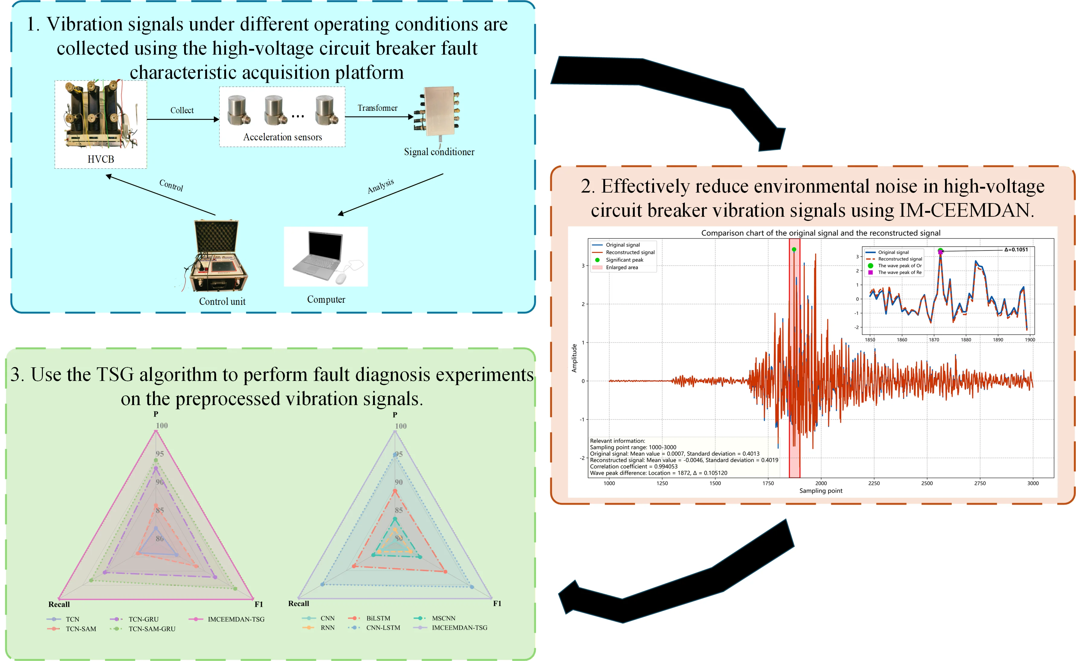
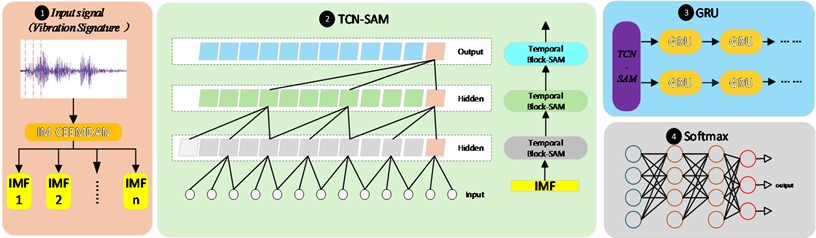
The workflow of the proposed model is shown in Fig. 1. The vibration signal of the HVCB is decomposed into several IMF components by CEEMDAN and screened through the Pearson correlation coefficient. Then, the screened IMF components are input into the TSG hybrid model through multiple channels for parallel computing to extract time series features. Finally, fault classification is carried out by the Softmax classifier. CEEMDAN with the Pearson correlation coefficient screening strategy introduced can more effectively and adaptively separate environmental noise. TCN uses causal convolution and residual networks to capture long-term dependencies of vibration signals. SAM applies attention weights to the features extracted by TCN, and the weighted features are input into GRU, which can further capture the short-term temporal relationship of the vibration signal.

Fig. 1The workflow of IMCEEMDAN-TSG

2.1. IMCEEMDAN signal denoising method

To remove the influence of environmental noise on the vibration signal from the original signal, a Pearson correlation coefficient screening strategy was used to improve CEEMDAN. Characteristic IMFs were determined by calculating the Pearson correlation coefficient between each IMF and the original signal, and noise was then removed.

2.1.1. CEEMDAN decomposition principle

CEEMDAN is an improved EMD method suitable for processing nonlinear and non-stationary signals. By adding adaptive noise to the vibration signal, performing multiple EMD decompositions on the noisy signal, and finally averaging all resultant IMF components from the decomposition, the modal aliasing phenomenon can be reduced, and the accuracy and stability of the decomposition can be improved [16]. First, adding different noise instances to the original signal $s (t)$ to generate a set of new signals:

1

s_{i} (t) = s (t) + n_{i} (t),

where $s_{i} (t)$ is the signal with added noise and $n_{i} (t)$ is the random noise instance.

Secondly, perform EMD decomposition on each noisy signal $s_{i} (t)$ to get a set of IMF components, and the calculation formula is:

2

s_{i} (t) = \sum_{k = 1}^{N} I_{i, k} (t) + r_{i} (t),

where $I_{i, k} (t)$ is the $k$ -th intrinsic mode function of the $i$ -th signal, $N$ is the number of IMF components, and $r_{i} (t)$ is the residual of the $i$ -th signal.

Then, all IMF component sets are average to derive the final intrinsic mode function:

3

I_{k}^{i} (t) = \frac{1}{M} \sum_{i = 1}^{M} I_{i, k} (t),

where $I_{k}^{i} (t)$ is the final $k$ -th intrinsic mode function, and $M$ is the number of noise instances.

2.1.2. Pearson correlation coefficient screening strategy

The Pearson correlation coefficient, also known as the Pearson product-moment correlation coefficient, can measure the linear correlation between the IMF components decomposed by the CEEMDAN denoising method and the original vibration signal and filter out the noise in the original vibration signal [26]. Its calculation formula is:

4

ρ_{X Y} = \frac{cov (X, Y)}{σ_{X} σ_{Y}} = \frac{E (X Y) - E (X) E (Y)}{\sqrt{E (X^{2}) - [E (X)]^{2}} \sqrt{E (Y^{2}) - [E (Y)]^{2}}} = \frac{n \sum_{i = 1}^{n} x_{i} y_{i} - (\sum_{i = 1}^{n} x_{i}) (\sum_{i = 1}^{n} y_{i})}{\sqrt{n \sum_{i = 1}^{n} x_{i}^{2} - {(\sum_{i = 1}^{n} x_{i})}^{2}} \sqrt{n \sum_{i = 1}^{n} y_{i}^{2} - {(\sum_{i = 1}^{n} y_{i})}^{2}}},

where $c o v (X, Y)$ is the covariance of $X$ and $Y$ , $σ_{X}$ and $σ_{Y}$ are the standard deviations of $X$ and $Y$ . The closer the value of $ρ_{X Y}$ is to 1, the stronger the correlation between the two sets of data.

2.2. TCN-SAM model principle

To further extract important vibration signal features from the IMF components decomposed by the CEEMDAN denoising method and capture the temporal relationships of the HVCB’s vibration signals, the IMF components decomposed by the CEEMDAN denoising method are fed into the TCN-SAM algorithm for parallel computation to improve diagnostic accuracy. Furthermore, when a HVCB fails, such as when the tripping and closing coils become loose, the vibration signal exhibits a strong transient nature. This places a high demand on feature extraction models that can efficiently locate local transient features when processing long sequences of data.

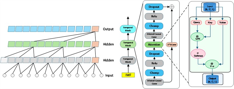
To meet these requirements, SAM is incorporated into the residual module of the TCN, aiming to improve the TCN’s processing capabilities for long sequences of data and its ability to focus on key features. The TCN-SAM model structure is shown in Fig. 2. SAM is inserted between two convolutional layers in the TCN’s Temporal Block module, enabling the model to focus on the important features extracted by the convolutional layers.

Fig. 2Structure diagram of TCN-SAM

2.2.1. Principle of TCN module

To solve the problem of gradient vanishing or gradient exploding in traditional deep learning models such as CNN and RNN, TCN provides stronger long-sequence causality and a more flexible receptive field. It uses convolutional neural networks to process sequence data, making it suitable for modeling long sequences [27]. The causal convolution of the TCN module strictly adheres to the temporal nature of the input sequence, for a one-dimensional time series $X = {x_{0}, x_{1}, . . ., x_{t}}$ and dilation coefficient $f = {0,1, 2, . . ., k - 1}$ :

5

H (T) = (X_{d}^{* k} f) (T) = \sum_{i = 0}^{k - 1} f (i) \cdot x_{T - d_{i}},

where $k$ represents the expansion coefficient and $d$ represents the expansion factor.

After adding causal convolution, the top layer of the TCN network can also receive feature information transmitted from the bottom layer, and the range is significantly improved compared to the previous receptive field size.

2.2.2. Self-attention mechanism (SAM)

In order to enable TCN to assign weights to vibration signal features when processing IMF components, SAM is added to the residual network of TCN to improve the model’s ability to extract important features of vibration signals.

SAM is a method that generates a contextual representation of each element by calculating the relationship between each position in the input sequence. Unlike traditional models such as RNN or LSTM, SAM allows the element at each position to interact directly with all other positions in the sequence, which makes it particularly suitable for processing long-distance dependencies [28].

Each element in the input sequence is mapped to a query vector $Q$ , a key vector $K$ , and a value vector $V$ through different weight matrices. $Q$ , $K$ , and $V$ corresponding to the input element $x_{i}$ are expressed as follows:

6

Q_{i} = W^{Q} x_{i}, ​ K_{i} = W^{K} x_{i}, ​ V_{i} = W^{V} x_{i} .

A scaling factor is usually introduced during calculation to scale the similarity between $Q$ and $K$ . Then normalized by the SoftMax function to obtain the attention weight of each position. The calculation formula is:

7

Attention (Q, K, V) = softmax (\frac{Q K^{T}}{\sqrt{d_{k}}}) V .

The value of Attention ( $Q$ , $K$ , $V$ ) represents the importance of sequence features and can give higher weights to important features, making the model more robust.

2.3. Principle of GRU module

The GRU layer is added after the TCN-SAM module to enhance the algorithm’s ability to capture dynamic correlation features between adjacent time steps of the vibration signal and optimize the model’s ability to extract local features. The GRU is a simplified version of the LSTM unit proposed by Cho et al. [13] and generally achieves comparable performance but with faster computation speed. Fig. 3 shows the basic architecture of the GRU unit.

Fig. 3Structure diagram of GRU unit

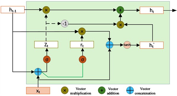
The working principle of the GRU structural unit is as follows: the update gate $(Z_{t})$ is responsible for adjusting the degree of integration of the current information with the hidden state at the previous moment to update the state of the hidden layer. The calculation formula of the update gate is shown in Eq. (8). The reset gate $(R_{t})$ is responsible for determining which information is retained from the current input and the past hidden state. The calculation formula of the reset gate is shown in Eq. (9). The current hidden layer $(h'_{t})$ state is shown in Eq. (10). The final hidden layer $(h_{t})$ state is shown in Eq. (11):

8

z_{t} = σ (W^{(z)} x_{t} + U^{(z)} h_{t - 1}),

9

r_{t} = σ (W^{(r)} x_{t} + U^{(r)} h_{t - 1}),

10

h'_{t} = \tan h (W x_{t} + r_{t} ⊙ U h_{t - 1}),

11

h_{t} = z_{t} ⊙ h_{t - 1} + (1 - z_{t}) ⊙ h'_{t} .

GRU does not clear the sequence information over time. It retains the relevant information and passes it to the next unit, effectively avoiding the gradient disappearance problem.

3. Simulated fault experimental setup

To verify the effectiveness and superiority of the proposed method, this section will design a systematic experimental scheme. First, Section 3.1 introduces the construction of the simulation experimental platform. Based on this, Section 3.2 elaborates on the simulated fault types and their settings. Finally, Section 3.3 presents a complete fault diagnosis process.

3.1. Simulated fault experiment platform

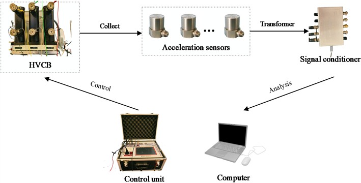
A fault simulation experimental platform was built based on the ZN63A-12/T1250-25(G) vacuum HVCB. The operating state of the HVCB was controlled by a switch’s mechanical characteristic tester. The acceleration sensors (sampling rate of 64 kHz) were used to collect vibration signals within 0.4 s intervals during multiple opening and closing operations of the HVCB under simulated fault conditions. The collected vibration signals were input into a host computer for signal processing and analysis via an MPS-HD2408 signal acquisition card. The simulated fault experimental platform is shown in Fig. 4.

Fig. 4The fault simulation experiment platform of HVCB

3.2. Simulation fault categories

Using the above fault simulation experimental platform of HVCB, vibration signals of five typical fault states of HVCB were collected, including normal working state, loosening of the closing coil, jamming of the core, jamming of the energy storage spring, loosening of the operating mechanism, and dry grinding of the transmission chain, with 200 samples for each state. The specific simulation conditions and the number of collected samples are shown in Table 1. During the acquisition of vibration signals on the fault simulation experimental platform, the background interference in the experimental environment is quite complex, and a large amount of random noise is mixed into the acquired vibration signals.

To facilitate the comparison of various operating conditions of the HVCB, Fig. 5 and Fig. 6 show the normal working state and the simulated fault state of the HVCB.

Table 1HVCB fault setting method

Label	Condition	Simulation method
F1	Normal	No fault
F2	Closing coil loose	Loosen the coil fixing nut
F3	Core stuck	Insulation tape-wrapped core
F4	Energy storage spring stuck	Foreign body placement
F5	Loose operating mechanism	Loosen the actuator nut
F6	Drive chain dry grinding	Reduce chain lubrication

3.3. Fault diagnosis procedure

The case study’s runtime environment included an Intel i5-12400f CPU, an RTX-4060Ti GPU, Python version 3.9, and PyTorch version 12.8 CUDA.

Fig. 5The normal operating state of the HVCB. Photo: Zhihui Yu, 15.04.2025, PuTian

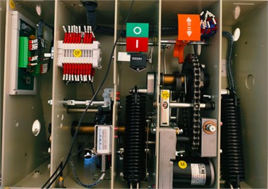
Fig. 6The classic fault states of HVCB. Photo by Zhihui Yu, 10.06.2025, PuTian

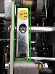
a) Closing coil loose

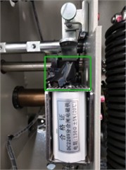
b) Core stuck

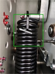
c) Energy storage spring stuck

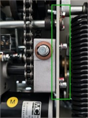
e) Loose operating mechanism

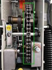
f) Drive chain dry grinding

Fig. 7 shows the fault diagnosis process. The vibration signals of HVCB collected on the simulation fault experiment platform are decomposed by CEEMDAN and then divided into a training set, a validation set, and a test set in a ratio of 7:2:1. The hyperparameters of IMCEEMDAN-TSG training are shown in Table 2. The training set and validation set are input into the TSG hybrid algorithm, and the model is trained by adjusting the network weight parameters. Finally, the performance of the trained model is tested on the test set. At the same time, an early stopping mechanism is added during the model training process. When the loss function does not decrease for five consecutive rounds, the model stops training to prevent overfitting.

4. Experimental results and analysis

This section designs several experiments to evaluate the performance of the proposed algorithm. The experiments first demonstrate and analyze the fault diagnosis results of the proposed algorithm for HVCB. Simultaneously, multiple ablation experiments were conducted to verify the effectiveness of its various mechanisms. Finally, the proposed algorithm was compared with several traditional and advanced deep learning algorithms to validate its advancement.

Fig. 7Fault diagnosis process

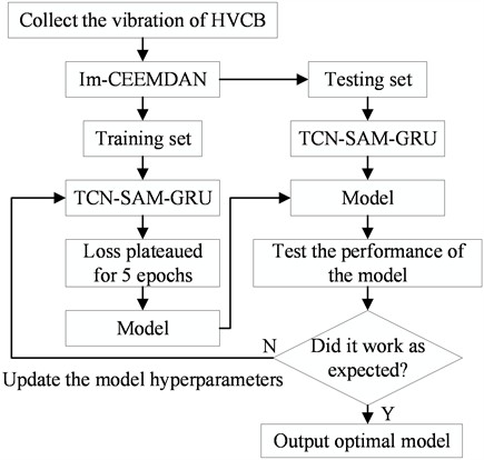
Table 2Model hyperparameter settings

Hyperparameters	Value	Hyperparameters	Value
Batch-Size	64	Learn-rater	0.001
Epochs	30	Optimizer	Adam
Sample	5	Dropout	0.3
Patience	3	Weight-decay	0.001

4.1. IMCEEMDAN decomposition of vibration signals

The HVCB typically operate in noisy environments, and their vibration signals contain noise or transient impacts. After the vibration signals are processed by IMCEEMDAN decomposition, noise reduction can be achieved by selectively filtering IMF components, thereby enhancing the robustness and generalization ability of the model. Fig. 8 shows the time-domain diagram of the HVCB’s vibration signal generated by the experimental platform under normal operating conditions.

Fig. 8Time-domain diagram of vibration signal of HVCB (Normal condition)

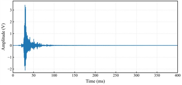
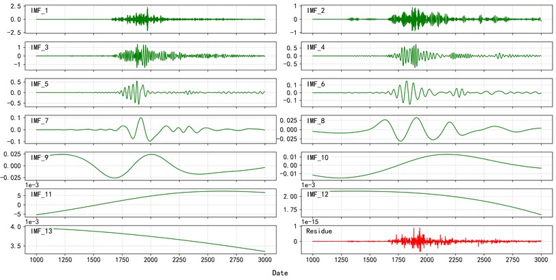
This signal is first decomposed by CEEMDAN into several IMF components and residuals as shown in Fig. 9, thereby reducing the volatility and complexity of the vibration signal data. In this case, the standard deviation of the added noise in the CEEMDAN algorithm is set to 0.2, and the number of iterations is set to 300. Fig. 9 presents the decomposition result of the vibration signal using the CEEMDAN algorithm. Since the vibration signal of the HVCB is a transient signal, the amplitude of the signal tends to be flat in the later stage. To facilitate the comparison of the differences between each IMF component and the residuals, only 1000-3000 data points are used for display.

In Fig. 9, IMF1-IMF13 are arranged in descending order of frequency and complexity. IMF1-IMF4 represents the most frequent and complex parts of the time series, which do not exhibit significant mode aliasing. As the number of IMF component sequences gradually decreases, the variation patterns become more intuitive.

Fig. 9CEEMDAN decomposition result (Normal condition)

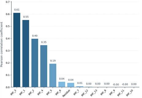
To compare the correlation degree between each IMF component and the original vibration signal, the Pearson correlation coefficient between the vibration signal and each IMF component after decomposition was calculated. Fig. 10 shows the decomposition result. The results show that the Pearson correlation coefficients between IMF1 and IMF3 and the original vibration signal are the highest, indicating that IMF1 and IMF3 are the main features of the original vibration signal. The Pearson correlation coefficients between IMF2, IMF4, and IMF5 and the original vibration signal are much higher than those of the remaining components, which are the secondary features of the original vibration signal.

Fig. 10Pearson correlation coefficient between IMF component and vibration signal

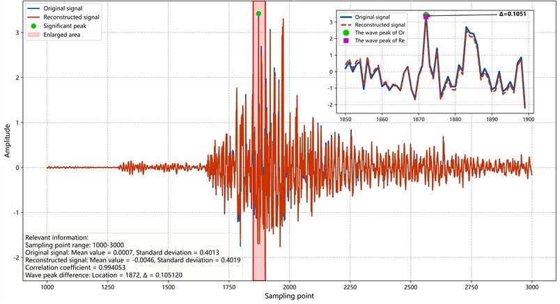
Irrelevant classifications with a Pearson correlation coefficient less than 0.2 were removed, and the components IMF1, IMF2, IMF3, IMF4, and IMF5 were superimposed and reconstructed. The reconstructed signal was compared with the original vibration signal, as shown in Fig. 11. The results show that the standard deviation between the reconstructed signal and the source vibration signal is 0.4013, the mean difference is 0.0007, and the Pearson correlation coefficient reaches 0.993. The reconstructed vibration signal and the original vibration signal have a high degree of similarity in overall level and fluctuation. Moreover, the difference at the highest peak of the two signals is only 0.1030, indicating that these five IMF components jointly characterize the main subset of significant attributes in the original source vibration signal. The reconstructed signal is relatively smooth, and the phase at the peak is aligned, achieving high-fidelity extraction of fault feature information.

Fig. 11Pearson correlation coefficient between IMF component and vibration signal

4.2. IMCEEMDAN-TSG model testing experiment

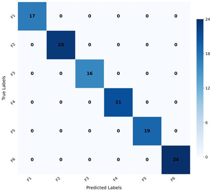
After the IMCEEMDAN decomposition algorithm decomposes the vibration signal, the TSG mixed model is used to extract the five IMF components after Pearson correlation coefficient screening to extract the main features. Table 3 shows the dimension changes of the IMF components after being processed by the TSG model. The features extracted by the model are used to identify the fault state and complete the fault diagnosis. Fig. 12 shows the confusion matrix of the diagnostic results. The experimental results show that the IMCEEMDAN-TSG model has a good diagnostic effect on the simulated fault data set of the HVCB, and the diagnostic accuracy can reach 100 %.

Table 3Model hyperparameter settings

Layers	Dimensionality	Layers	Dimensionality
Input signal	[64, 5, 25600]	Adjustment	[64, 25600, 128]
TCN Block1	[64, 32, 25600]	GRU1	[64, 25600, 128]
TCN Block2	[64, 64, 25600]	GRU2	[64, 25600, 128]
TCN Block3	[64, 128, 25600]	Classification	[64, 6]

Fig. 12IMCEEMDAN-TSG model test results

4.3. Compared with other methods

This experiment conducted multiple ablation experiments and comparative tests on the proposed algorithm. First, the Pearson correlation coefficient screening strategy was applied to the EMD, EEMD, and CEEMDAN decomposition methods for comparison. Second, a controlled variable method was used on the TSG hybrid model to verify the rationality and necessity of the improvement strategy by gradually removing key modules from the model. Finally, the proposed algorithm was compared horizontally with several classic and cutting-edge algorithms on the same dataset, and its superiority was verified through multiple evaluation metrics.

4.3.1. Comparative experiment of different decomposition methods

The Pearson correlation coefficients between the IMF components obtained after processing the vibration signals with EMD, EEMD, and CEEMDAN denoising methods and the original signals were calculated separately. The IMF components with higher values were used to construct the reconstructed signal by superposition, and the SNR and NCC values were calculated. The results are shown in Table 4. Since the EMD and EEMD denoising methods are affected by the endpoint effect of the vibration signal during decomposition, endpoint oscillations occur, resulting in errors when determining the peak of the wave. The results show that among the signal indicators generated under the same reconstruction method, the NCC of the CEEMDAN denoising method is 0.9910, which is 0.0046 higher than that of the EMD denoising method and 0.2687 higher than that of the EEMD denoising method. And the SNR of the CEEMDAN denoising method is 1.7476, which is higher than that of the EMD denoising method and is much higher than that of the EEMD denoising method.

Table 4Model hyperparameter settings

Metrics	EMD	EEMD	CEEMDAN
SNR	15.6450	0.4792	17.3926
NCC	0.9864	0.7223	0.99101

4.3.2. Ablation experiment

To further verify the effectiveness of the IMCEEMDAN-TSG model, it was compared with the combined models such as TCN, TCN-SAM, TCN-GRU, and TSG. Fig. 13(a) presents the results of this experiment. The results show that the diagnostic accuracy of the IMCEEMDAN-TSG model reaches 100 %, and the F1 score and recall rate are all close to 1. The accuracy, F1 score, and recall rate of the combined models, such as TCN, TCN-SAM, TCN-GRU, and TSG, are all lower than those of the proposed model.

Compared with single TCN, TCN-SAM adds the attention mechanism to the causal convolution and residual network of TCN, enabling the model to extract the important features of the vibration signal by freely allocating weights. The TCN-GRU model integrates the long-term dependencies of the signals extracted by TCN through GRU, improving the model’s extraction efficiency for non-stationary signals. Meanwhile, the TSG model possesses the advantages of both TCN-SAM and TCN-GRU, not only being able to reallocate the feature weights of the vibration signal through the long-term dependencies of the signals extracted by TCN after the self-attention mechanism but also being able to model the complex temporal relationships and nonstationarity through GRU, comprehensively enhancing the efficiency and robustness of the model’s feature extraction.

Fig. 13Comparison of evaluation indicators of different models

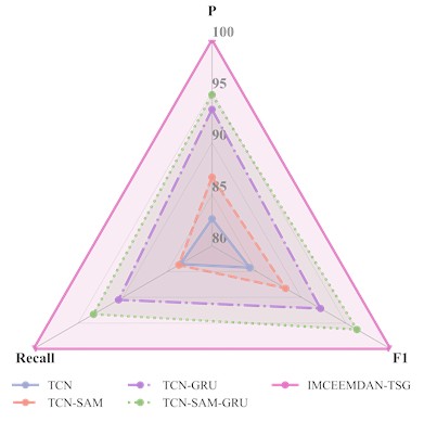
a) Ablation experiment

b) Comparative experiment

4.3.3. Comparative experiment

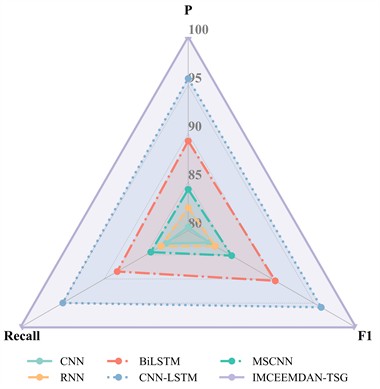
The development of deep learning has broken the limitations of traditional fault diagnosis, which relies heavily on signal processing experts for manual feature extraction, and has greatly improved the efficiency of diagnosis under massive data. To verify the advancement of the proposed model, it is compared with methods such as CNN [29], RNN [30], BiLSTM [31], CNN-LSTM [32], and MSCNN [33]. The comparison results are shown in Fig. 13(b).

When the CNN model processes one-dimensional vibration signals, due to the limitations of its receptive field, this network has difficulty capturing the early transient characteristics of the HVCB’s vibration signals. When the RNN model is used to extract the features of vibration signals, it is prone to experiencing gradient explosion, which may affect the diagnostic accuracy. The BiLSTM model is very sensitive to the input at each time step. Noise in the original signal accumulates continuously during each loop, causing a severe shift in the extracted features. The CNN-LSTM hybrid model fails to effectively integrate the vibration features and the temporal features when extracting the important features of the HVCB’s vibration signals. The MSCNN model is suitable for processing stationary signals, but its performance is not ideal when processing non-stationary signals such as vibration signals from HVCB.

Therefore, based on the experimental results, it can be concluded that compared with the IMCEEMDAN-TSG model, the above-mentioned traditional models have poor performance in extracting the characteristics of the vibration signals of HVCB and are unable to complete the fault diagnosis of HVCB effectively.

5. Conclusions

This paper proposes an IMCEEMDAN-TSG deep learning classification method, which can not only reduce the impact of environmental noise on vibration signals but also capture the temporal relationship of the HVCB’s vibration signals to improve the fault diagnosis accuracy of HVCB. First, the vibration signal is decomposed into IMFs to separate the environmental noise through the CEEMDAN algorithm with the Pearson correlation coefficient screening strategy. Secondly, TCN is used to capture the long-term relationship of the vibration signal, and SAM is added to TCN to enable the algorithm to freely allocate feature weights and reduce the impact of noise on the important features of the vibration signal. Then, the GRU algorithm further captures the short-term relationship of the vibration signal. Finally, the extracted important features are input into the classifier to classify the operating status of the equipment and complete the fault diagnosis. The experimental results show that the classification effect evaluation indicators such as accuracy, F1 score, and recall rate of the HVCB simulation fault data set of this method reached 100 %, 0.98, and 0.99, which are all improved compared with other traditional methods.

At present, this method still has many challenges to face:

1) This method only uses the vibration signal of the HVCB for fault diagnosis. Using a single signal may not accurately reflect the operating status of the equipment.

2) It is difficult to obtain a large number of vibration signals covering various circuit breaker types, different operating conditions, and different failure modes in real time with accurate annotations. However, a large amount of data is required when training the IMCEEMDAN-TSG hybrid model.

3) Although this method performs well in tests on the HVCB fault simulation dataset, it cannot explain its physical meaning.

In the future, we will conduct targeted research to address the challenges faced by this method.

References

R. Li, Y. Hu, X. Wang, B. Zhang, and H. Chen, “Estimating the impacts of a new power system on electricity prices under dual carbon targets,” Journal of Cleaner Production, Vol. 438, p. 140583, Jan. 2024, https://doi.org/10.1016/j.jclepro.2024.140583

Publisher
M. Mohammadhosein, K. Niayesh, A. A. Shayegani-Akmal, and H. Mohseni, “Online assessment of contact erosion in high voltage gas circuit breakers based on different physical quantities,” IEEE Transactions on Power Delivery, Vol. 34, No. 2, pp. 580–587, Apr. 2019, https://doi.org/10.1109/tpwrd.2018.2883208

Publisher
A. Asghar Razi-Kazemi and K. Niayesh, “Condition monitoring of high voltage circuit breakers: past to future,” IEEE Transactions on Power Delivery, Vol. 36, No. 2, pp. 740–750, Apr. 2021, https://doi.org/10.1109/tpwrd.2020.2991234

Publisher
K. Obarcanin and B. Lacevic, “Methods for condition assessment of the high voltage circuit breakers based on vibration fingerprint-a survey,” IEEE Access, Vol. 13, pp. 86542–86552, Jan. 2025, https://doi.org/10.1109/access.2025.3570000

Publisher
Q. Song, J. Wang, Q. Song, K. Li, W. Hao, and H. Jiang, “Fault diagnosis of HVCB via the subtraction average based optimizer algorithm optimized multi channel CNN-SABO-SVM network,” Scientific Reports, Vol. 14, No. 1, p. 29507, Nov. 2024, https://doi.org/10.1038/s41598-024-80954-6

Publisher
Q. Yang, J. Ruan, Z. Zhuang, D. Huang, and Z. Qiu, “A new vibration analysis approach for detecting mechanical anomalies on power circuit breakers,” IEEE Access, Vol. 7, pp. 14070–14080, Jan. 2019, https://doi.org/10.1109/access.2019.2893922

Publisher
Z. Chen, K. Zhang, L. Yang, and Y. Liang, “ANFIS based sound vibration combined fault diagnosis of high voltage circuit breaker (HVCB),” Energy Reports, Vol. 9, pp. 286–294, May 2023, https://doi.org/10.1016/j.egyr.2022.12.130

Publisher
Y. Tan, E. Hu, Y. Liu, J. Li, and W. Chen, “Review of digital vibration signal analysis techniques for fault diagnosis of high-voltage circuit breakers,” IEEE Transactions on Dielectrics and Electrical Insulation, Vol. 31, No. 1, pp. 404–418, Feb. 2024, https://doi.org/10.1109/tdei.2023.3339114

Publisher
M. Demetgul, K. Yildiz, S. Taskin, I. N. Tansel, and O. Yazicioglu, “Fault diagnosis on material handling system using feature selection and data mining techniques,” Measurement, Vol. 55, pp. 15–24, Sep. 2014, https://doi.org/10.1016/j.measurement.2014.04.037

Publisher
T. Li, Y. Zhao, C. Zhang, J. Luo, and X. Zhang, “A knowledge-guided and data-driven method for building HVAC systems fault diagnosis,” Building and Environment, Vol. 198, p. 107850, Jul. 2021, https://doi.org/10.1016/j.buildenv.2021.107850

Publisher
K. Yildiz, E. Güneş, and A. Bas, “CNN-based gender prediction in uncontrolled environments,” Düzce Üniversitesi Bilim ve Teknoloji Dergisi, Vol. 9, No. 2, pp. 890–898, Apr. 2021, https://doi.org/10.29130/dubited.763427

Publisher
A. Sherstinsky, “Fundamentals of recurrent neural network (RNN) and long short-term memory (LSTM) network,” Physica D: Nonlinear Phenomena, Vol. 404, p. 132306, Mar. 2020, https://doi.org/10.1016/j.physd.2019.132306

Publisher
K. Cho et al., “Learning phrase representations using RNN encoder-decoder for statistical machine translation,” in Proceedings of the 2014 Conference on Empirical Methods in Natural Language Processing (EMNLP), pp. 1724–1734, Jan. 2014, https://doi.org/10.3115/v1/d14-1179

Publisher
J. F. Kolen and S. C. Kremer, “Gradient flow in recurrent nets: the difficulty of learning LongTerm dependencies,” A Field Guide to Dynamical Recurrent Networks, pp. 237–243, Jan. 2009, https://doi.org/10.1109/9780470544037.ch14

Publisher
C. Qin, L. Chen, Z. Cai, M. Liu, and L. Jin, “Long short-term memory with activation on gradient,” Neural Networks, Vol. 164, pp. 135–145, Jul. 2023, https://doi.org/10.1016/j.neunet.2023.04.026

Publisher
Z. Zhou, J. Zhang, R. Cheng, Y. Rui, X. Cai, and L. Chen, “Improving purity of blasting vibration signals using advanced empirical mode decomposition and wavelet packet technique,” Applied Acoustics, Vol. 201, p. 109097, Dec. 2022, https://doi.org/10.1016/j.apacoust.2022.109097

Publisher
H. Jiang, C. Li, and H. Li, “An improved EEMD with multiwavelet packet for rotating machinery multi-fault diagnosis,” Mechanical Systems and Signal Processing, Vol. 36, No. 2, pp. 225–239, Apr. 2013, https://doi.org/10.1016/j.ymssp.2012.12.010

Publisher
X. Shang et al., “Research on fault diagnosis of UAV rotor motor bearings based on WPT-CEEMD-CNN-LSTM,” Machines, Vol. 13, No. 4, p. 287, Mar. 2025, https://doi.org/10.3390/machines13040287

Publisher
W. Zhang, Z. Qu, K. Zhang, W. Mao, Y. Ma, and X. Fan, “A combined model based on CEEMDAN and modified flower pollination algorithm for wind speed forecasting,” Energy Conversion and Management, Vol. 136, pp. 439–451, Mar. 2017, https://doi.org/10.1016/j.enconman.2017.01.022

Publisher
C. Junsheng, Y. Dejie, and Y. Yu, “Research on the intrinsic mode function (IMF) criterion in EMD method,” Mechanical Systems and Signal Processing, Vol. 20, No. 4, pp. 817–824, May 2006, https://doi.org/10.1016/j.ymssp.2005.09.011

Publisher
P. J. J. Luukko, J. Helske, and E. Räsänen, “Introducing libeemd: a program package for performing the ensemble empirical mode decomposition,” Computational Statistics, Vol. 31, No. 2, pp. 545–557, Jul. 2015, https://doi.org/10.1007/s00180-015-0603-9

Publisher
M. E. Torres, M. A. Colominas, G. Schlotthauer, and P. Flandrin, “A complete ensemble empirical mode decomposition with adaptive noise,” in IEEE International Conference on Acoustics, Speech and Signal Processing (ICASSP), pp. 4144–4147, May 2011, https://doi.org/10.1109/icassp.2011.5947265

Publisher
J. Zhang, Y. Wang, J. Tang, J. Zou, and S. Fan, “MS-TCN: a multiscale temporal convolutional network for fault diagnosis in industrial processes,” in American Control Conference (ACC), pp. 1601–1606, May 2021, https://doi.org/10.23919/acc50511.2021.9482728

Publisher
X. Ye, J. Yan, Y. Wang, L. Lu, and R. He, “A novel capsule convolutional neural network with attention mechanism for high-voltage circuit breaker fault diagnosis,” Electric Power Systems Research, Vol. 209, p. 108003, Aug. 2022, https://doi.org/10.1016/j.epsr.2022.108003

Publisher
A. Kumar, A. Parey, and P. K. Kankar, “A new hybrid LSTM-GRU model for fault diagnosis of polymer gears using vibration signals,” Journal of Vibration Engineering and Technologies, Vol. 12, No. 2, pp. 2729–2741, May 2023, https://doi.org/10.1007/s42417-023-01010-7

Publisher
Y. Gao, Y. Hang, and M. Yang, “A cooling load prediction method using improved CEEMDAN and Markov Chains correction,” Journal of Building Engineering, Vol. 42, p. 103041, Oct. 2021, https://doi.org/10.1016/j.jobe.2021.103041

Publisher
J. Zhan, C. Wu, X. Ma, C. Yang, Q. Miao, and S. Wang, “Abnormal vibration detection of wind turbine based on temporal convolution network and multivariate coefficient of variation,” Mechanical Systems and Signal Processing, Vol. 174, p. 109082, Jul. 2022, https://doi.org/10.1016/j.ymssp.2022.109082

Publisher
Y. Ding, M. Jia, Q. Miao, and Y. Cao, “A novel time-frequency Transformer based on self-attention mechanism and its application in fault diagnosis of rolling bearings,” Mechanical Systems and Signal Processing, Vol. 168, p. 108616, Apr. 2022, https://doi.org/10.1016/j.ymssp.2021.108616

Publisher
Z. Huang, L. Wang, Q. Ge, Y. Chen, and D. Zhang, “An intelligent fault diagnosis method for CNN-SVM circuit breaker based on quantum particle swarm optimization,” in Journal of Physics: Conference Series, Vol. 2113, No. 1, p. 012047, Nov. 2021, https://doi.org/10.1088/1742-6596/2113/1/012047

Publisher
H. Liu, J. Zhou, Y. Zheng, W. Jiang, and Y. Zhang, “Fault diagnosis of rolling bearings with recurrent neural network-based autoencoders,” ISA Transactions, Vol. 77, pp. 167–178, Jun. 2018, https://doi.org/10.1016/j.isatra.2018.04.005

Publisher
B. Song, Y. Liu, J. Fang, W. Liu, M. Zhong, and X. Liu, “An optimized CNN-BiLSTM network for bearing fault diagnosis under multiple working conditions with limited training samples,” Neurocomputing, Vol. 574, p. 127284, Mar. 2024, https://doi.org/10.1016/j.neucom.2024.127284

Publisher
J. Zhang, J. Gao, and B. Wang, “CNN-LSTM based circuit breaker fault prediction model research,” in 6th International Conference on Energy Systems and Electrical Power (ICESEP), pp. 1491–1494, Jun. 2024, https://doi.org/10.1109/icesep62218.2024.10651674

Publisher
C. Peng, H. Li, W. Gui, Z. Tang, and X. Yuan, “Fault diagnosis method for rotating machinery based on MSCNN-MGAT,” IEEE Transactions on Instrumentation and Measurement, Vol. 74, pp. 1–11, Jan. 2025, https://doi.org/10.1109/tim.2025.3587368

Publisher

About this article

Received

December 17, 2025

Accepted

March 11, 2026

Published

April 16, 2026

SUBJECTS

Fault diagnosis based on vibration signal analysis

DOI

https://doi.org/10.21595/jve.2026.25923

Keywords

HVCB

vibration signal

deep learning

fault diagnosis

Acknowledgements

This research was funded by the National Natural Science Foundation of China (Grant No. 52577115), Key Technological Innovation Focus and Industrialization Projects in Fujian Province (2024G029), the Zhejiang Office of Philosophy and Social Science (25NDJC129YB), and the Startup Fund for Advanced Talents of Putian University (2023133).

Data Availability

The datasets generated during and/or analyzed during the current study are available from the corresponding author on reasonable request.

Author Contributions

Zhihui Yu: Conceptualization, Investigation, Methodology, Software, Writing - Original Draft Preparation. Chuan Lin: Data Curation, Funding Acquisition, Methodology, Project administration, Validation, Supervision, Writing - Review and Editing. Chaohui Huang: Visualization, Supervision. Yifan Huang: Data Curation, Investigation. Jiaman Luo: Formal Analysis, Validation.

Conflict of interest

The authors declare that they have no conflict of interest.

This is an open access article distributed under the Creative Commons Attribution License, which permits unrestricted use, distribution, and reproduction in any medium, provided the original work is properly cited.