Abstract
Compressors serve as fundamental power units in underground natural gas storage facilities and frequently need to accommodate wide-range operational condition adjustments. However, their inherent nonlinear characteristics, coupled with high-noise and uncertain operating environments, pose significant challenges to precise control and safe operation. To accurately predict compressor operational status and provide reliable decision-making information for operation and maintenance, this study proposes an operating-state prediction method for gas storage compressors based on vibration-sequence analysis and a Bidirectional Long Short-Term Memory (BiLSTM) network. Singular Spectrum Analysis (SSA) is first applied to decompose and reconstruct monitoring signals, extracting dominant trend components while suppressing background noise. A Convolutional Neural Network (CNN) is subsequently employed to capture multi-scale local features, after which the BiLSTM network learns temporal evolution patterns from the extracted features. The Adam optimizer is utilized to enhance training stability and prediction accuracy. Experimental validation using real monitoring data from gas storage compressors indicates that the proposed method achieves precise and reliable prediction of compressor operating states.
Highlights
- A hybrid deep learning framework (SSA-CNN-BiLSTM) is proposed for accurate compressor state prediction under noisy, nonlinear operating conditions.
- Singular Spectrum Analysis with K-means clustering automatically extracts trend components and suppresses noise, eliminating subjective threshold selection.
- The method achieves superior prediction performance on real gas storage compressor vibration data, outperforming LSTM, BiLSTM, and CNN-BiLSTM baselines.
1. Introduction
As vital energy infrastructure, underground natural gas storage facilities deliver essential functions including seasonal peak shaving, emergency supply during incidents, and strategic reserve capacity. These capabilities render storage installations indispensable for maintaining the security and stability of natural gas supply systems [1]. As the key power equipment within such systems, compressors operate under complex and highly variable conditions. These include frequent transitions between injection and withdrawal, broad pressure-regulation ranges, and significant fluctuations in flow rate [2]. These factors impose stringent challenges on precise control and safe operation of compressors, making them more susceptible to destabilization, surge, and other destructive risks during operation [3].
Effective monitoring and accurate prediction of compressor operating states are essential for provide reliable decision-making to ensure safe and reliable operation. However, monitoring signals from gas storage compressors typically exhibit strong nonlinearity, non-stationarity, high noise levels, and abrupt changes. These characteristics make accurate prediction of compressor operational status challenging. Traditional state-monitoring features, such as frequency-domain indicators or time-domain statistical metrics, are often insufficient to characterize the dynamic evolution of compressor conditions, thereby limiting the accuracy of fault warning and life prediction [4, 5].
Data-driven modeling approaches, particularly artificial neural networks, have shown strong capability in capturing nonlinear patterns and learning hidden representations from monitoring data. Through training, these models can effectively identify underlying trends in equipment behavior and provide reliable predictions of operating-state changes [6-8]. Consequently, neural-network-based methods have been widely applied to condition modeling and state prediction of various mechanical systems [9]. For instance, Wan et al. [10] realized condition monitoring and fault diagnosis of compressors using a 1D-CNN. Zhang et al. [11] implemented intelligent fault diagnosis for compressors using a Convolutional Deep Belief Network. Tian et al. [12] integrated continual learning theory with compressor systems to achieve dynamic monitoring of operational status. Zhong et al. [13] further demonstrated that neural networks can accurately predict compressor performance under off-design operating conditions.
Although these studies have demonstrated the effectiveness of neural-network-based methods for equipment state prediction, individual model architectures have inherent limitations [14]. Different models excel in different aspects, such as feature extraction or temporal modeling, but no single model can fully capture the multi-scale characteristics of complex industrial signals. As a result, their performance often degrades when dealing with strongly nonlinear and non-stationary data [15]. To overcome these limitations, recent studies have explored hybrid prediction models that combine the strengths of different neural architectures [16, 17]. Pu et al. [18] implemented compressor condition monitoring by integrating LSTM with an attention mechanism. Wu et al. [19] verified the effectiveness of combining time-delayed Feedforward Neural Networks (FFNN) with LSTM for compressor load forecasting. More recently, Siddique et al. [20] proposed a hybrid fault-diagnosis framework for milling cutting tools that integrates time-frequency analysis with a dual-branch encoder architecture, achieving high diagnostic accuracy under noisy conditions. Umar et al. [21] developed a burst-informed acoustic emission framework that captures short, high-energy fracture-related transients and links them directly to damage progression, enabling explainable failure diagnosis in milling operations.
Nevertheless, whether using standalone or hybrid neural models, the prevalence of high noise levels in industrial monitoring signals remains a major challenge. Noise can significantly obscure underlying state changes and reduce prediction accuracy. As a result, increasing attention has been given to combining signal-denoising techniques with neural-network-based prediction frameworks. For example, Dao et al. [22] achieved fault diagnosis for power station hydraulic turbines using a Bayesian optimized CNN-LSTM hybrid architecture. Lian et al. [23] combined wavelet denoising with Support Vector Machines (SVMFH) to enhance wind power forecasting. Ding [24] applied the 3σ criterion to preprocess raw sensor data and then developed a Deep Convolutional Neural Network (DCNN) model, achieving high-precision bearing state prediction.
To achieve operational status monitoring of gas storage compressors, we proposed a hybrid prediction model. This model is tailored to the nonlinear, non-stationary, and noise-contaminated characteristics of compressor monitoring signals in underground gas storage facilities. The model integrates Singular Spectrum Analysis (SSA), CNN, and BiLSTM. SSA is used to extract trend and periodic components while suppressing noise, with K-means clustering incorporated to improve component selection. CNN is then applied to capture local non-stationary patterns in the signals, and BiLSTM is employed to model nonlinear temporal dependencies, enabling accurate prediction of compressor operating states. By integrating signal processing techniques with neural networks, the proposed approach enhances overall learning capability and improves robustness against noise.
The proposed SSA-CNN-BiLSTM framework has the following fundamental innovations:
1) Automated trend extraction via SSA with K-means clustering, which intelligently identifies principal components based on statistical features, eliminating subjective threshold selection.
2) Functionally differentiated architecture where SSA extracts global trends, CNN captures local non-stationary patterns, and BiLSTM models bidirectional temporal dependencies – each component playing a distinct and complementary role.
3) Domain-tailored design with parameters physically matched to compressor characteristics and optimized for vibration signal patterns.
4) Comprehensive validation on real industrial data from operational gas storage compressors, demonstrating practical applicability beyond benchmark datasets.
The remainder of this paper is organized as follows. Section 2 introduces the fundamental methodologies employed in this study, including SSA, CNNs, and BiLSTM. Section 3 elaborates on the proposed SSA-CNN-BiLSTM trend knowledge learning model, detailing the procedures for signal decomposition, trend extraction, and data preprocessing. Section 4 presents the experimental setup, dataset description, preprocessing steps, and a comprehensive analysis of the results, including comparisons with other benchmark models. Finally, Section 5 concludes the paper by summarizing the key findings and discussing potential directions for future research.
2. Methods
2.1. Singular spectrum analysis
SSA is a non-parametric time-series analysis technique that effectively extracts trend, periodic, and noise components from raw monitoring signals. The method first transforms the original sequence into a Hankel matrix. Singular Value Decomposition (SVD) is then applied to obtain a set of decomposed components. These components can be selectively reconstructed to retain meaningful information.
To begin, a sliding window and diagonal averaging are used to convert the time-series data into a Hankel matrix. SVD is then performed on this matrix, yielding the left singular vectors, singular values, and right singular vectors. By selecting the dominant singular values and their corresponding vectors, the key components of the original sequence can be reconstructed.
As a data-driven denoising and decomposition method, SSA separates the main trend components from low-energy, unstructured noise components. The trend components are typically represented by the first few high-energy singular values. This process enables different frequency elements within the signal to be isolated, while retaining only the principal components to reconstruct a cleaner signal with an improved signal-to-noise ratio.
2.2. Convolutional neural networks
CNNs are a type of feedforward neural network widely used for feature extraction in time-series analysis. The core principle of CNNs is to apply convolution kernels along the input sequence to capture features at different scales.
Fig. 1Flowchart of 1D CNN for time series processing
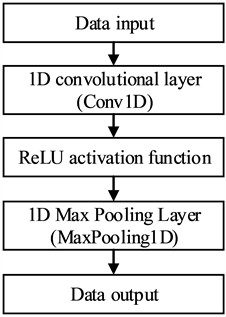
In this study, the raw time-series data are first passed through one-dimensional convolution layers to extract local temporal features. A ReLU activation function is then applied to introduce nonlinearity and enhance feature expressiveness. Subsequently, a max-pooling layer reduces the dimensionality of the feature maps while preserving the most informative components. The processed feature representations are then forwarded to subsequent network layers for further analysis and prediction. The flowchart of 1D-CNN for time series processing used in this study is shown in Fig. 1.
2.3. Bidirectional long short-term memory networks
LSTM networks are a specialized form of Recurrent Neural Networks (RNNs). They are designed to address the vanishing-gradient and exploding-gradient problems commonly encountered when modeling long-term temporal dependencies. LSTMs achieve this by introducing memory cells and gating mechanisms that regulate the flow of information. The memory cell stores long-term information, while the input, forget, and output gates determine how much information is added, retained, or released at each time step.
In a LSTM unit, the input gate controls the extent to which new information enters the memory cell, the forget gate determines how much historical information is preserved, and the output gate regulates how the internal state contributes to the next layer. This structure enables LSTMs to effectively capture long-range dependencies within sequential data. The structure of a LSTM unit is presented in Fig. 2.
Fig. 2The structure of a LSTM unit
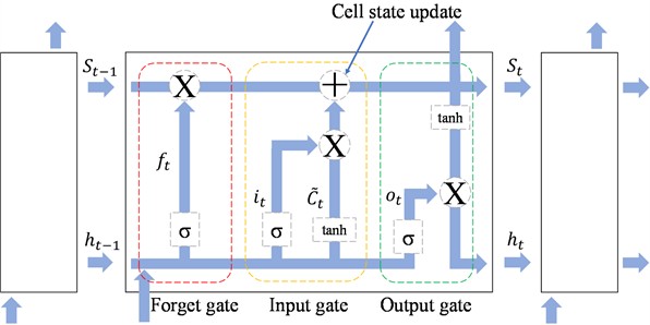
The training of an LSTM model usually adopts the Back Propagation Through Time (BPTT) algorithm, which is similar to the classical Back Propagation (BP) algorithm. When dealing with long sequences, BPTT is prone to gradient vanishing or gradient explosion, and LSTMs alleviate this problem effectively through the gating mechanism.
Fig. 3Flowchart of the BiLSTM neural network
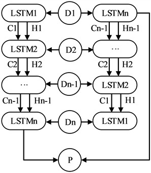
BiLSTM is an extension of the standard LSTM. A BiLSTM layer consists of two LSTM layers: one processes the sequence in the forward direction from beginning to end, and the other processes it in the backward direction from end to beginning. At each time step, the hidden states from the forward and backward LSTMs are concatenated or summed to obtain the final hidden state. While a standard LSTM can only use past information, a BiLSTM can exploit both past and future information, and therefore provides better performance for modeling and predicting time-series signals. A schematic diagram of the BiLSTM layer structure is shown in Fig. 3.
3. Trend knowledge learning model based on SSA-CNN-BiLSTM
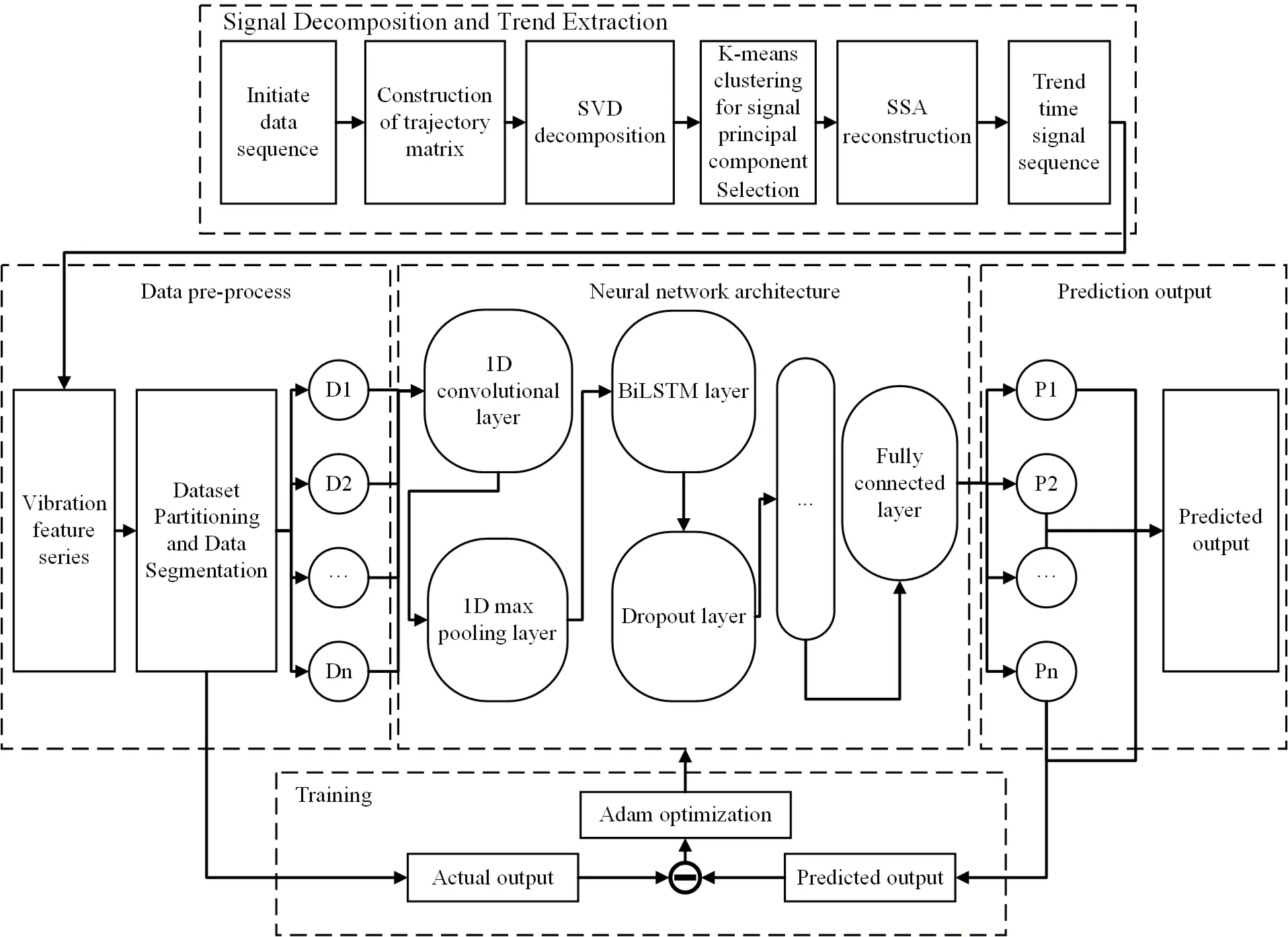
Since compressor vibration, temperature, and other monitoring signals exhibit the characteristics of continuous time-series data, this study establishes a trend knowledge learning model based on SSA-CNN-BiLSTM. The overall workflow of the model is shown in Fig. 4.
Fig. 4Flowchart of the SSA-CNN-BiLSTM model
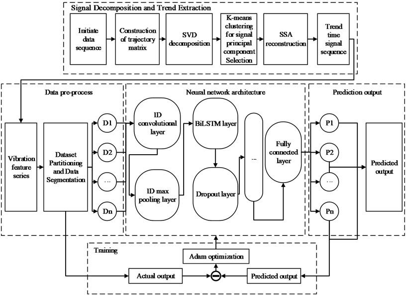
For compressors, rotor vibration is a concentrated reflection of their operational status. The use of eddy current sensors to measure vibration displacement within the same shaft cross-section near the bearing housing is a standard configuration for compressor monitoring. Therefore, extracting features from vibration displacement signals to form time series, and leveraging CNN and LSTM to extract and integrate spatial and temporal information, can effectively predict the operational state of the compressor.
In this model, the raw time-series data are first decomposed using SSA to separate the trend component from noise, after which the trend component is selected for model training to high-light the dominant characteristics of the signal. In the data preprocessing stage, the extracted trend sequence is standardized and training samples are constructed using a sliding-window approach.
The model training stage adopts a hybrid architecture composed of a 1D-CNN and BiLSTM network, while Dropout and L2 regularization are incorporated to mitigate over-fitting. During training, the Adam optimizer is employed to iteratively update the model parameters. Once optimized, the model is applied to the test dataset to generate predictions, which are evaluated using some metrics to provide a comprehensive assessment of predictive performance. After iterative training, the model ultimately achieves accurate prediction of compressor vibration, enabling condition prediction for gas storage compressors.
3.1. Signal decomposition and trend extraction
The raw data sequence is first processed by the trend-extraction module to obtain the trend component used for model training. The original time-series signal is expressed as:
where represents the data points in time step . This time-series sequence serves as the fundamental dataset for training the model.
A suitable window length is selected to construct the trajectory matrix , which is defined as follows:
where . For a time-series of length , is typically chosen to be proportional to the dominant periodicity but not exceeding to ensure a sufficient number of lagged vectors (). SVD is then applied, yielding the following factorization:
where is the matrix of left singular vectors, is the diagonal matrix containing the singular values, and is the matrix of right singular vectors. After SVD, can be expressed as the sum of several rank-one matrices:
where denotes the singular value, and are the th columns of the left and right singular vector matrices, respectively.
To extract the trend component, the first one or several components with the largest singular values are typically selected for reconstruction. The reconstructed trajectory matrix is then converted back into the form of the original time series through diagonal averaging.
To enable automatic identification and selection of the principal components and further enhance the intelligence of SSA analysis, the K-means clustering algorithm is introduced to cluster the reconstructed components obtained from decomposition. For each reconstructed component, features such as variance and the value of the autocorrelation function are extracted to form feature vectors. These vectors are then clustered using the K-means algorithm, grouping components with similar statistical characteristics into the same cluster. The number of clusters is set to 2, corresponding to a “principal component cluster” and a “noise cluster.” Components representing dominant trends or significant periodic structures are assigned to the “principal component” cluster, whereas components with low energy and lacking periodic structure are categorized as “noise.” Finally, by reconstructing the components belonging to the principal cluster, the useful information in the time series is effectively preserved, achieving automatic extraction of trend and periodic features while suppressing noise. This binary choice directly implements the theoretical separation in SSA between a few dominant components capturing signal dynamics and numerous low-energy components representing noise, without introducing unnecessary complexity or requiring subjective threshold selection.
The training and prediction module are responsible for model training and iterative updating of network parameters. First, the loss between the theoretical output and the actual output is computed. Then, the Adam optimizer is used to update the model parameters, and convergence is accelerated through early stopping and learning rate scheduling mechanisms. As iterative training progresses, the model parameters are continuously adjusted to minimize the loss function, thereby gradually improving prediction performance.
3.2. Data preprocessing
The data preprocessing module prepares the input sequence for neural-network processing. The extracted trend sequence is divided into training and testing subsets according to a predefined ratio. Specifically, the first portion of the sequence is used as the training set:
while the remaining portion is used as the test set:
3.3. State prediction
The constructed CNN-BiLSTM neural network model is employed to process the time-series data and generate prediction results. First, a one-dimensional convolution (Conv1D) layer is applied to the input time-series signal to capture local temporal features. After convolution, a ReLU activation function is used to introduce nonlinearity and preserve the nonlinear characteristics of the signal. The resulting feature maps are then passed to a MaxPooling1D layer, which performs downsampling to reduce dimensionality and retain the most salient information.
The extracted feature maps are subsequently fed into Bidirectional Long Short-Term Memory (BiLSTM) layers. The BiLSTM architecture captures bidirectional temporal dependencies, enabling the network to learn relationships from both past and future contexts. To prevent overfitting, a Dropout layer is incorporated after the BiLSTM layer, randomly discarding a portion of neurons to enhance generalization capability. Another BiLSTM layer followed by a Dropout layer is then applied to further strengthen the model’s ability to learn complex temporal patterns. Finally, a fully connected layer maps the output of the BiLSTM network to the prediction space.
4. Experiments
Experimental validation of the proposed BiLSTM model was conducted using monitoring signals collected from underground gas storage compressors. The dataset includes multiple types of time-series measurements, such as temperature time signals, displacement time signals, pressure time signals, and liquid level time signals.
4.1. Experimental environment
Python was used as the programming language for the experiments, and the neural network algorithms, including LSTM and BiLSTM, were implemented using the TensorFlow framework. The experiments were conducted on a computation station with 11th Gen Intel(R) Core(TM) i7-11700 processor and 16 GB of RAM.
4.2. Dataset
The dataset used in this study consists of time-series monitoring signals collected from gas storage compressors. The experimental validation of the proposed BiLSTM model was conducted using monitoring signals collected from operational gas storage compressors. The collected dataset includes multiple types of time-series measurements, such as temperature-time signals, displacement-time signals, and pressure-time signals. Two representative displacement signals were selected for model validation and comparison: the motor non-drive-end terminal displacement (MNDTD) signal, as shown in Fig. 5(a), and the motor drive-end terminal displacement (MDTD) signal, as shown in Fig. 5(b). Both MNDTD and MDTD are time-series signals that reflect the displacement variations of the drive-end and non-drive-end terminals during compressor operation. The monitoring sequences contain approximately 130,000 data points per channel, collected over a continuous operational period at a sampling rate of 2 kHz, covering multiple operating phases including startup, steady-state operation, load variation, and shutdown. This diversity of signal types and operating phases demonstrates the richness of the dataset, and while this study focuses on displacement signals as the primary indicators of mechanical condition, the proposed method can be readily extended to other signal types.
4.3. Data preprocessing
The historical MNDTD and MDTD monitoring sequences contain approximately 130,000 data points. To improve computational efficiency while preserving representative system behavior, an 8,000-point segment was selected for analysis. Since the region around the 20,000th sampling point reflects a stable displacement state during compressor start-up, the segment beginning at the 19,000th point was extracted. The selection was to avoid the initial startup transients (approximately the first 15,000-18,000 points) and focus on the region where the compressor has reached relatively stable operating conditions, as evidenced by the consistent vibration amplitude range in Fig. 5(a). This ensures that the model learns patterns representative of normal operational behavior rather than transient startup dynamics. This interval avoids the noise-dominated regions at the beginning and end of the signal and retains the essential dynamic characteristics relevant for forecasting. The red circle in Fig. 5(a) marked the extracted segment MNDTD.
In K-means clustering, we set number of clusters 2. Convergence is achieved when either: (a) the change in cluster centroids between consecutive iterations falls below 10-4, or (b) the maximum number of iterations (set to 300) is reached. This ensures stable and reproducible clustering outcomes.
In preparing the experimental data, it is essential to determine an appropriate window length for the SSA decomposition, as the window size directly influences both the number and the characteristics of the decomposed components, thereby affecting the model’s ability to capture meaningful trend and periodic structures. 100 is selected as it provides adequate resolution to capture cycle-related periodic behavior while maintaining statistical reliability . This choice enables effective separation of the trend component from background noise, as validated by the subsequent prediction performance. Meanwhile, quantitative indicators such as Mean Squared Error (MSE) and Mean Absolute Percentage Error (MAPE) were employed to evaluate the discrepancy between the reconstructed and original signals.
The model handles different categories of input data in a consistent manner. When only a single sequence variable (e.g. MNDTD) is used, each prediction step yields a single output value. When multiple types of monitoring data are incorporated, such as displacement, temperature, and humidity, the model is capable of learning cross-dependencies among variables and producing multi-output predictions simultaneously. This enables the framework to adapt to both univariate and multivariate forecasting scenarios while leveraging the complementary information contained in heterogeneous monitoring signals.
Fig. 5Schematic diagram of original vibration signals for MNDTD and MDTD
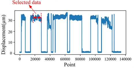
a) MNDTD
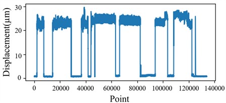
b) MDTD
4.4. Experimental results analysis
The training process begins by feeding the data into the model. Before conducting full experiments, the model structure must be optimized. In this study, a controlled-variable approach is used to adjust and compare the effects of the time-window length and the number of BiLSTM layers on model performance.
First, with the network structure fixed at two BiLSTM layers, different window sizes (10, 20, and 50) were evaluated. The results are shown in Table 1. When the window size was set to 20, the model achieved the lowest MAPE and RMSE values on the test set, indicating the highest prediction accuracy. Therefore, a window size of 20 was selected for subsequent experiments.
Table 1Experimental results with different window sizes and 2-Layer BiLSTM
Window | Train | Test | ||||
MAPE | RMSE | MAPE | RMSE | |||
10 | 1.3344 % | 0.5271 | 0.7721 | 1.3317 % | 0.5324 | 0.7911 |
20 | 1.3254 % | 0.5241 | 0.7747 | 1.3230 % | 0.5298 | 0.7931 |
50 | 1.3289 % | 0.5289 | 0.7704 | 1.3330 % | 0.5358 | 0.7882 |
The neural network input window of 20 time steps, selected through the empirical optimization in Table 1, also has a physical basis. With the same sampling rate of 10 kHz and rotational frequency of 50-100 Hz, a 20-point window corresponds to 10 % to 20 % of a full mechanical rotation. This window size captures local vibration patterns such as instantaneous acceleration, velocity changes, and short-term fluctuations within a fraction of a rotation. It provides sufficient temporal resolution to detect meaningful local dynamics while remaining short enough to enable rapid response to changing compressor conditions.
After determining a window size of 20, a data segment with a length of 1000 points was extracted to evaluate the effect of BiLSTM depth. Models with 2, 3, 4, and 5 BiLSTM layers were tested, with each BiLSTM layer followed by a Dropout layer with a dropout rate of 20 %. The results are presented in Table 2.
It can be observed that increasing the number of BiLSTM layers does not lead to significant improvements in MAPE, RMSE, or . This indicates that deeper architectures bring limited benefits once sufficient temporal features have been learned and may even introduce a risk of overfitting. Therefore, two BiLSTM layers were selected as the final model configuration.
Table 2Experimental results with window size of 20 and different BiLSTM layers
Number of layers | Train | Test | ||||
MAPE | RMSE | MAPE | RMSE | |||
2 | 1.2111 % | 0.4800 | 0.8110 | 1.2535 % | 0.5034 | 0.8132 |
3 | 1.2158 % | 0.4867 | 0.7942 | 1.2737 % | 0.5276 | 0.8004 |
4 | 1.2169 % | 0.4778 | 0.8108 | 1.2500 % | 0.5087 | 0.8158 |
5 | 1.2175 % | 0.4837 | 0.8244 | 1.2547 % | 0.5175 | 0.8192 |
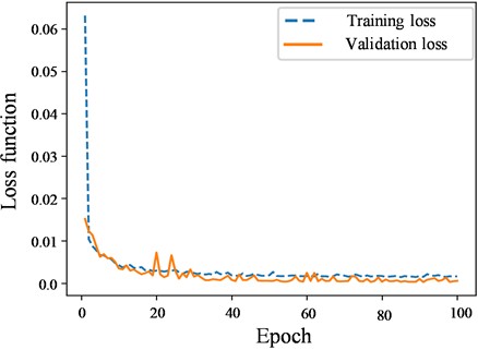
With a window size of 20 and a BiLSTM depth of two layers, the model training was conducted. The variation of the loss values during training is shown in Fig. 6. As the number of iterations increased, the loss values on both the training and validation sets steadily decreased and gradually converged to a stable level after approximately 20 iterations.
Fig. 6Iteration loss plot of the SSA-CNN-BiLSTM model
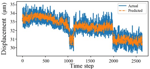
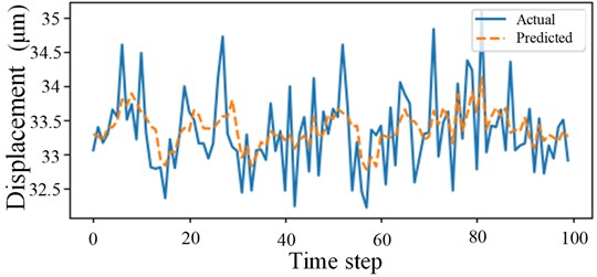
The prediction results after model training are shown in Fig. 7(a) illustrates the model’s performance on a sequence of 2,500 data points, while 7(b) provides a zoomed-in view of the first 100 data points for detailed comparison.
After 500 training iterations, the model achieved MAPE values below 2% on both the training and test sets, RMSE values below 0.5, and values above 0.8, demonstrating strong predictive performance. The results are shown in Table 3.
Table 3Experimental results of BiLSTM model
Train | Test | ||||
MAPE | RMSE | MAPE | RMSE | ||
1.2391 % | 0.4930 | 0.8006 | 1.2414 % | 0.4998 | 0.8159 |
To further evaluate model performance, the proposed SSA-CNN-BiLSTM model was compared against three alternative approaches. These included a CNN-BiLSTM model without trend decomposition, a BiLSTM-only model, and a traditional LSTM model. In the comparative experiments, all CNNs we applied shared the same architecture: one convolutional layer, each followed by a max-pooling layer, with 64 filters per layer, a kernel size of 3, and a stride value of 1.
Since missing values or abnormal points may occur during the acquisition and transmission of experimental data, and noise components are also present in the signals, a moving average method is applied for noise reduction when SSA is not used to extract noise. The formula of the moving average method is as follows:
where denotes the window size and represents the index of the current data point.
Fig. 7Prediction results of the SSA-CNN-BiLSTM model
a)
b)
To apply the moving average method, an appropriate window size must first be selected. The window size determines how many neighboring points are used to compute each averaged value. For each point in the sequence, the average of the surrounding points (including itself) within the selected window is calculated and used as the smoothed value of that point. In this study, the window size is set to 3, meaning that every three points are averaged.
The training results of each model are presented in Table 4. The LSTM model achieves a lower MAPE on the training set (1.2826 %) than the CNN-BiLSTM and BiLSTM models. However, its value on the test set (0.7562) is relatively low, indicating insufficient generalization ability. Further verification shows that under complex operating conditions, the LSTM model struggles to consistently capture the nonlinear dynamic behavior of the signal. The CNN-BiLSTM and BiLSTM models exhibit relatively lower overall performance, but still demonstrate certain predictive capability. The CNN-BiLSTM model obtains a MAPE of 1.3473 % on the test set, while the BiLSTM model achieves 1.3307 %. Although their values are comparatively lower, both remain within an acceptable range, suggesting that these models retain adequate capability in feature extraction and trend representation. In contrast, the SSA-CNN-BiLSTM model achieves the lowest MAPE values on both the training and test sets (1.2391 % and 1.2414 %, respectively), indicating the smallest relative prediction error. Meanwhile, the model achieves the highest value on the test set (0.8159), showing the best agreement between predicted and actual values among all models. In addition, the RMSE of this model is also relatively low, further confirming its superior performance in complex time-series prediction tasks.
From the comparison results, it can be observed that the convolution operations in CNN enable the extraction of local patterns and non-stationary features, allowing the CNN-BiLSTM model to outperform the standalone BiLSTM model. This enhances the model’s feature representation capability and improves its understanding of local dependencies within the signal.
On the other hand, SSA plays a significant role in the overall model. By performing trend extraction and noise separation, SSA effectively removes most noise components while preserving essential nonlinear variations, resulting in a smoother and more informative signal. This process substantially improves the model’s sensitivity to the underlying data and enhances prediction accuracy.
The experimental results indicate that the proposed SSA-CNN-BiLSTM model can accurately and effectively predict the operating state of gas storage compressors.
Table 4Comparison of experimental results for different models under identical parameters
Model | Number of layers | Dimension | Train | Test | ||||
MAPE | RMSE | MAPE | RMSE | |||||
SSA-CNN-BiLSTM | 1 lyaer CNN 2 layer BiLSTM | Filters = 64 128×2 | 1.24 % | 0.493 | 0.80 | 1.24 % | 0.50 | 0.82 |
CNN-BiLSTM | 1 lyaer CNN 2 layers BiLSTM | Filters = 64 128×2 | 1.36 % | 0.535 | 0.78 | 1.35 % | 0.54 | 0.78 |
BiLSTM | 2 layers BiLSTM | 128×2 | 1.34 % | 0.530 | 0.77 | 1.33 % | 0.53 | 0.78 |
LSTM | 2 layers BiLSTM | 128×2 | 1.28 % | 0.509 | 0.77 | 1.27 % | 0.51 | 0.76 |
The experimental design in Table 4 also serves as an ablation study to evaluate the individual contribution of each component. Removing SSA by comparing SSA-CNN-BiLSTM against CNN-BiLSTM increases test MAPE from 1.24 % to 1.35 %, a degradation of 0.11 percentage points. This confirms that SSA preprocessing plays a critical role in noise suppression and trend extraction. Adding CNN without SSA preprocessing, as seen by comparing CNN-BiLSTM with BiLSTM, yields minimal improvement with MAPE values of 1.35 % versus 1.33 %. This suggests that feature extraction alone is insufficient without proper denoising. Interestingly, BiLSTM achieves a MAPE of 1.33 %, which underperforms compared to standard LSTM at 1.27 %, indicating that bidirectional processing is not always beneficial for vibration time-series data. Nevertheless, the full SSA-CNN-BiLSTM model achieves the best overall performance with a MAPE of 1.24 %, demonstrating that the synergistic combination of all components rather than any single component is responsible for the observed improvements.
To rigorously validate the performance improvements of the proposed SSA-CNN-BiLSTM model, we conducted statistical significance testing using paired t-tests across 10 independent runs with different random initializations. As shown in Table 5, the proposed model achieves statistically significant improvements over the CNN-BiLSTM and BiLSTM baselines ( 0.01), confirming that the integration of SSA preprocessing and the CNN feature extractor provides genuine performance benefits beyond random variation. The improvement over the LSTM baseline, while positive, does not reach statistical significance at the 95 % confidence level ( 0.087), indicating that the performance difference is modest for this particular comparison. These results provide strong statistical evidence for the effectiveness of our proposed approach while also highlighting areas for future investigation.
Table 5Statistical significance test results comparing SSA-CNN-BiLSTM with baseline models
Comparison | Mean MAPE difference | Dimension | p-value |
SSA-CNN-BiLSTM vs. CNN-BiLSTM | –0.11 % | 4.231 | 0.0021 |
SSA-CNN-BiLSTM vs. BiLSTM | –0.09 % | 3.872 | 0.0036 |
SSA-CNN-BiLSTM vs. LSTM | –0.03 % | 1.923 | 0.0870 |
To provide a more comprehensive performance context, we additionally compared our proposed model against Support Vector Regression (SVR), a representative non-deep learning method widely used for time-series prediction. The SVR model was implemented with an RBF kernel, and hyperparameters were optimized via grid search with 5-fold cross-validation. The optimal configuration (100, 0.01, 0.1) was then evaluated on the same test set used for the deep learning models.
The optimized SVR model achieved a test MAPE of 1.52 %, with corresponding RMSE of 0.61 and of 0.71. This performance is notably weaker than all deep learning approaches, which achieved MAPE values ranging from 1.24 % to 1.35 %. Specifically, the proposed SSA-CNN-BiLSTM model outperforms SVR by a substantial margin of 0.28 percentage points in MAPE, representing an 18.4 % relative improvement. These results confirm that deep learning methods are better suited for capturing the complex nonlinear patterns in compressor vibration signals, while also further validating the effectiveness of our proposed approach.
From a practical deployment perspective, the proposed SSA-CNN-BiLSTM model demonstrates strong potential for real-time industrial applications. With a total inference time of approximately 8.5 ms per prediction on standard hardware, the model can easily meet the real-time requirements of compressor condition monitoring, where predictions at 1-2 second intervals are sufficient. For long-term deployment, model accuracy can be maintained through periodic retraining (e.g., monthly) or performance-triggered updates when prediction errors exceed predefined thresholds. Regarding edge computing feasibility, the model's compact size (~1.2 MB) enables deployment on resource-constrained devices such as the Raspberry Pi 4 (inference time ~45 ms) or NVIDIA Jetson Nano (~12 ms), both well within practical latency limits. Future work will explore model quantization and pruning techniques to further optimize deployment on industrial edge devices, as well as incremental learning strategies for continuous model adaptation without full retraining.
5. Conclusions
This study presents a novel compressor operation state prediction method that integrates SSA, CNN, and BiLSTM networks to address the challenges of nonlinear dynamics and background noise under complex operating conditions in underground gas storage compressors. Experimental validation using real monitoring signals confirms the effectiveness of the proposed model.
In the SSA-CNN-BiLSTM framework, SSA facilitates effective decomposition and reconstruction of raw signals, enabling the extraction of dominant features while substantially mitigating the impact of background noise on prediction performance. The CNN component captures multi-scale local patterns in the signals, while the BiLSTM module learns their temporal dependencies and dynamic evolution. This integrated architecture allows the model to effectively represent nonlinear dynamic behavior under varying operational conditions and achieve accurate prediction of compressor monitoring signals.
The experimental results demonstrate that the proposed method exhibits strong predictive performance for compressor operational signals. The model provides reliable decision support for safe compressor operation and energy-efficiency optimization, while also offering valuable insights for condition monitoring and fault diagnosis in underground gas storage compressor systems.
From a practical deployment perspective, the proposed SSA-CNN-BiLSTM model demonstrates strong potential for real-time industrial applications. With a total inference time of approximately 8.5 ms per prediction on standard hardware, the model can easily meet the real-time requirements of compressor condition monitoring. For long-term deployment, model accuracy can be maintained through periodic retraining or performance-triggered updates when prediction errors exceed predefined thresholds. Regarding edge computing feasibility, the model’s compact size enables deployment on resource-constrained devices. Future work will explore model quantization and pruning techniques to further optimize deployment on industrial edge devices, as well as incremental learning strategies for continuous model adaptation without full retraining.
Despite its strong performance, this study has several limitations. First, while the model was validated on data from a single compressor unit, its scalability to different compressor types remains to be further investigated. Second, long-term performance drift due to component aging or environmental changes was not addressed, highlighting the need for continuous model adaptation strategies. Third, while real-time feasibility was demonstrated on edge devices, practical deployment constraints such as system integration and bandwidth limitations require validation in actual industrial settings. Future work will also focus on multi-compressor validation, online learning for drift adaptation, and real-world deployment testing.
References
-
Y. Wang, Z. Jiang, J. Zhang, C. Zhou, and W. Liu, “Performance analysis and optimization of reciprocating compressor with stepless capacity control system under variable load conditions,” International Journal of Refrigeration, Vol. 94, pp. 174–185, Oct. 2018, https://doi.org/10.1016/j.ijrefrig.2018.07.013
-
X. Gao and Y. Liu, “Design, modeling and characteristics research of a novel self-air-cooling reciprocating compressor,” International Journal of Refrigeration, Vol. 128, pp. 62–70, Aug. 2021, https://doi.org/10.1016/j.ijrefrig.2021.03.007
-
S. Ullah, M. F. Siddique, and J.-M. Kim, “Multi-sensor observer-based residual learning with Auto-Permutation Feature Importance for fault diagnosis of multistage centrifugal pumps under variable pressures,” Scientific Reports, Vol. 15, No. 1, p. 45735, Dec. 2025, https://doi.org/10.1038/s41598-025-32726-z
-
A. Kumar, “Research overview and prospect in condition monitoring of compressors,” Expert Systems with Applications, Vol. 277, p. 127284, Jun. 2025, https://doi.org/10.1016/j.eswa.2025.127284
-
Q. Lv, X. Yu, H. Ma, J. Ye, W. Wu, and X. Wang, “Applications of machine learning to reciprocating compressor fault diagnosis: A review,” Processes, Vol. 9, No. 6, p. 909, May 2021, https://doi.org/10.3390/pr9060909
-
X. Zhang, N. Xu, W. Dai, G. Zhu, and J. Wen, “Turbofan engine health prediction model based on ESO-BP neural network,” Applied Sciences, Vol. 14, No. 5, p. 1996, Feb. 2024, https://doi.org/10.3390/app14051996
-
P. Mobtahej, X. Zhang, M. Hamidi, and J. Zhang, “An LSTM-Autoencoder architecture for anomaly detection applied on compressors audio data,” Computational and Mathematical Methods, Vol. 2022, pp. 1–22, Sep. 2022, https://doi.org/10.1155/2022/3622426
-
F. Ochando, J. I. Guerrero, J. Luque, and C. Leon, “Engine and oil condition analysis using a hybrid supervised model with a multilayer neural network and expert rules,” IEEE Transactions on Industrial Informatics, Vol. 20, No. 10, pp. 11731–11739, Oct. 2024, https://doi.org/10.1109/tii.2024.3413296
-
B. G. Joung, C. Nath, Z. Li, and J. W. Sutherland, “Bearing anomaly detection in an air compressor using an LSTM and RNN-based machine learning model,” The International Journal of Advanced Manufacturing Technology, Vol. 134, No. 7-8, pp. 3519–3530, Sep. 2024, https://doi.org/10.1007/s00170-024-14322-z
-
A. Wan et al., “Fault diagnosis of air conditioning compressor bearings using wavelet packet decomposition and improved 1D-CNN,” Next Energy, Vol. 9, p. 100424, Oct. 2025, https://doi.org/10.1016/j.nxener.2025.100424
-
Y. Zhang and J. Ji, “Intelligent fault diagnosis of a reciprocating compressor using mode isolation convolutional deep belief networks,” IEEE/ASME Transactions on Mechatronics, Vol. 26, No. 3, pp. 1668–1677, Jun. 2021, https://doi.org/10.1109/tmech.2020.3027912
-
H. Tian, Y. Kang, Z. Li, K. Li, and H. Wang, “An adaptive continual learning framework for dynamic condition monitoring of reciprocating compressors,” Measurement Science and Technology, Vol. 36, No. 11, p. 116201, Nov. 2025, https://doi.org/10.1088/1361-6501/ae10cd
-
L. Zhong, R. Liu, X. Miao, Y. Chen, S. Li, and H. Ji, “Compressor performance prediction based on the interpolation method and support vector machine,” Aerospace, Vol. 10, No. 6, p. 558, Jun. 2023, https://doi.org/10.3390/aerospace10060558
-
Q. Zhang, X. Wei, Y. Wang, and C. Hou, “Convolutional neural network with attention mechanism and visual vibration signal analysis for bearing fault diagnosis,” Sensors, Vol. 24, No. 6, p. 1831, Mar. 2024, https://doi.org/10.3390/s24061831
-
X. Li, S. Zhou, F. Wang, and L. Fu, “An improved sparrow search algorithm and CNN-BiLSTM neural network for predicting sea level height,” Scientific Reports, Vol. 14, No. 1, p. 4560, Feb. 2024, https://doi.org/10.1038/s41598-024-55266-4
-
Y. Wang, Z. Xiao, D. Liu, J. Chen, D. Liu, and X. Hu, “Degradation trend prediction of hydropower units based on a comprehensive deterioration index and LSTM,” Energies, Vol. 15, No. 17, p. 6273, Aug. 2022, https://doi.org/10.3390/en15176273
-
G. Li, S. Guo, X. Li, and C. Cheng, “Short-term forecasting approach based on bidirectional long short-term memory and convolutional neural network for regional photovoltaic power plants,” Sustainable Energy, Grids and Networks, Vol. 34, p. 101019, Jun. 2023, https://doi.org/10.1016/j.segan.2023.101019
-
L. Pu, L. Zhang, J. Liu, and L. Qiu, “Industrial compressor-monitoring data prediction based on LSTM and self-attention model,” Processes, Vol. 13, No. 2, p. 474, Feb. 2025, https://doi.org/10.3390/pr13020474
-
D.-C. Wu, B. Bahrami Asl, A. Razban, and J. Chen, “Air compressor load forecasting using artificial neural network,” Expert Systems with Applications, Vol. 168, p. 114209, Apr. 2021, https://doi.org/10.1016/j.eswa.2020.114209
-
M. F. Siddique, W. Zaman, M. Umar, J.-Y. Kim, and J.-M. Kim, “A hybrid deep learning framework for fault diagnosis in milling machines,” Sensors, Vol. 25, No. 18, p. 5866, Sep. 2025, https://doi.org/10.3390/s25185866
-
M. Umar, M. F. Siddique, and J.-M. Kim, “Burst-informed acoustic emission framework for explainable failure diagnosis in milling machines,” Engineering Failure Analysis, Vol. 185, p. 110373, Mar. 2026, https://doi.org/10.1016/j.engfailanal.2025.110373
-
F. Dao, Y. Zeng, and J. Qian, “Fault diagnosis of hydro-turbine via the incorporation of Bayesian algorithm optimized CNN-LSTM neural network,” Energy, Vol. 290, p. 130326, Mar. 2024, https://doi.org/10.1016/j.energy.2024.130326
-
L. Lian and K. He, “Wind power prediction based on wavelet denoising and improved slime mold algorithm optimized support vector machine,” Wind Engineering, Vol. 46, No. 3, pp. 866–885, Oct. 2021, https://doi.org/10.1177/0309524x211056822
-
H. Ding, L. Yang, Z. Cheng, and Z. Yang, “A remaining useful life prediction method for bearing based on deep neural networks,” Measurement, Vol. 172, p. 108878, Feb. 2021, https://doi.org/10.1016/j.measurement.2020.108878
About this article

This work has been supported by Oil and Gas Major Project of China (Grant No. 2025ZD1401600).
The datasets generated during and/or analyzed during the current study are available from the corresponding author on reasonable request.
Hua Chen: conceptualization, methodology, resources, writing-review and editing, supervision and project administration. Liang Wang: formal analysis, methodology, software, investigation and visualization. Shuang Li: software, validation and writing-review and editing. Xiaohan Wei: resources, data curation, writing-original draft preparation and funding acquisition.
The authors declare that they have no conflict of interest.
