Analytical method for studying free vibrations of round plates on a non-homogeneous elastic foundation

Krutii, Yurii; Perperi, Alla; Kachmar, Roman; Predko, Rostyslav; Velychko, Danylo

doi:10.21595/mme.2026.26028

Mathematical Models in Engineering

Browse Journal

Submit article

Published: June 30, 2026

Check for updates

Analytical method for studying free vibrations of round plates on a non-homogeneous elastic foundation

Yurii Krutii¹

Alla Perperi²

Roman Kachmar³

Rostyslav Predko⁴

Danylo Velychko⁵

^{1, 2, 5}Odessa State Academy of Civil Engineering and Architecture, Odessa, Ukraine

^{3, 4}Lviv Polytechnic National University, Lviv, Ukraine

Corresponding Author:

Danylo Velychko

Cite the article Download PDF

Downloads 29

Abstract

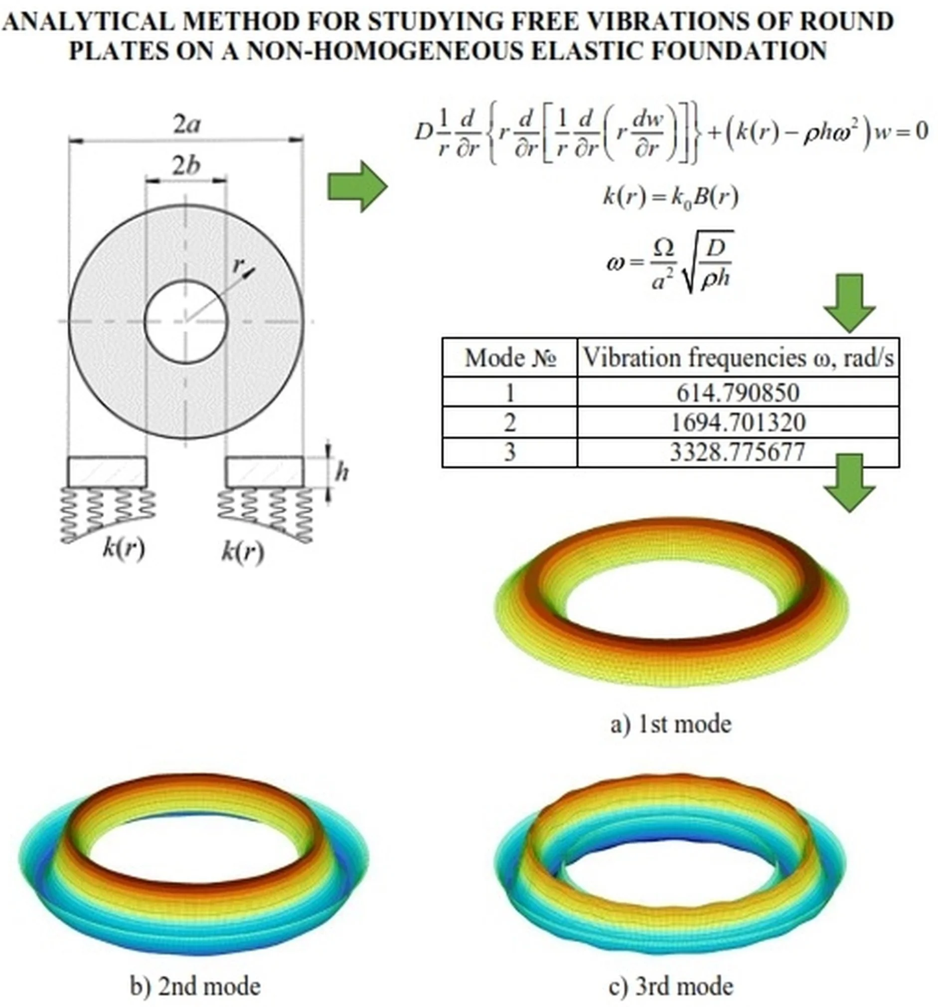
Free axisymmetric vibrations of a circular plate resting on an inhomogeneous, continuous elastic Winkler foundation are investigated. The foundation inhomogeneity is represented by a spatially varying subgrade modulus, which may be described by an arbitrary continuous function. For this class of structures, an analytical modal analysis method based on an exact solution of the governing partial differential equation is proposed. Numerical results for a circular plate are presented in tabulated form. To validate the proposed approach, the results are compared with those obtained from finite element analysis using the LIRA-FEM software package.

1. Introduction

Oscillatory phenomena are ubiquitous in nature and play a fundamental role across various fields of science and engineering, in particular in civil and industrial engineering [1]-[4], hydraulic engineering [5], mechanical engineering [6]-[8], and aerospace applications [9], [10].

In contemporary construction practice, circular plate elements supported by elastic foundations are widely utilized as essential structural components. Modal analysis of circular plates supported by inhomogeneous Winkler foundations is particularly relevant to soil-structure interaction problems and vibration control. These models are essential for the design and dynamic assessment of circular foundations, raft and pile caps, machine and turbine bases, pavements, manhole covers, storage tanks, and landing platforms for wind turbines and aerospace vehicles, where soil properties are inherently nonuniform. Accurate prediction of natural frequencies and mode shapes enables resonance avoidance, enhances structural safety, and supports material optimization.

Among the various approaches for modeling foundation-structure interaction, the Winkler model remains one of the most widely used. It represents the foundation as a system of independent vertical springs characterized by a single parameter, the subgrade modulus. In its simplest form, the foundation is assumed homogeneous, yielding a constant subgrade modulus and significantly simplifying the governing differential equations for plate vibrations. However, this idealization rarely reflects actual ground conditions, and more realistic analyses require consideration of foundation heterogeneity [11]. In such cases, the subgrade modulus varies spatially, which substantially increases the mathematical complexity of the problem and generally necessitates the use of approximate solution techniques.

The theory of circular plates is comprehensively presented in classical monographs [12]-[14]. In contrast, analytical solutions for circular plates resting on variable Winkler foundations remain scarce in the literature [11], [15], [16]. In particular, [15] and [16] develop analytical approaches for axisymmetric bending of circular plates supported by Winkler-type foundations with spatially varying stiffness, based on the general integral of the governing differential equation with variable coefficients.

In [17], the authors address this problem by employing the Rayleigh-Schmidt approach, presenting tabulated frequency coefficients for the lower symmetric and asymmetric transverse vibration modes of a thin isotropic plate, under the condition of elastic constraints against both displacement and rotation. Paper [18] proposes a generalized numerical method based on the classical Mohr method, adapted to analyze structures on a variable single-parameter elastic foundation. Notably, the method is formulated for efficient computer implementation. In [19], the lowest natural frequency of transverse vibrations of circular plates with fixed and simply supported edges was evaluated using the Rayleigh-Ritz variational approach. The trial functions employed consisted of polynomial terms, which conform to the boundary conditions at the plate’s perimeter, combined with trigonometric functions. The authors [20] used an analytical method to obtain the frequency equation of a circular plate with elastic edge supports, part of which rests on a discontinuous elastic foundation. Parametric investigations were performed to examine the response of circular plates with elastic edge supports, considering various values of the transverse stiffness and foundation parameters under different boundary conditions. In [21], a finite element-based numerical procedure is proposed for conducting nonlinear dynamic analysis of circular reinforced concrete slab structures subjected to variable dynamic loads. In article [22], free vibrations are investigated and modal analysis of thin circular plates with arbitrary boundary conditions is performed. The Pasternak and Winkler models are used to simulate the elastic base. The natural frequencies and vibration modes of circular plates are obtained using a numerical method for solving differential equations. The influence of the base stiffness parameters and boundary conditions on the natural frequencies and vibration modes is taken into account. Studies [23], [24] are dedicated to the study of vibrations of circular plates with unusual boundary conditions. Article [23] provides a study of the vibrational characteristics of thin circular plates on a homogeneous Winkler foundation with rotational elastic boundary condition at the edge. The frequency equation was obtained using an analytical method. Parametric studies of the vibrations of circular plates were carried out for different parameters of the stiffness of the elastic boundary condition on the contour. In [24], plate with the boundary conditions which deviate from the classical cases is considered. The transverse vibrations of thin circular plates on a homogeneous Winkler foundation with guided edge were investigated. Article [25] provides a study of the dynamics of thin circular plates fixed along the contour and performs a finite element analysis. By analyzing the dynamic behavior of the plate, the modes of vibrations are determined, which can be used to identify patterns characterizing the location of damage. In [26], exact solution is derived for the characteristics of free vibrations of thin circular plates, elastically constrained from displacement, resting on a Winkler elastic foundation. For circular plates constrained along their outer contour, parametric studies were conducted to assess the effect of the stiffness of the elastic foundation on the natural frequencies. Studies [27] and [28] investigate the application of the two-dimensional differential transformation method to analyze the dynamic response of functionally inhomogeneous circular plates resting on a Pasternak elastic foundation. Paper [29] considers the analysis of free vibrations of circular plates supported by Winkler and Pasternak types of subgrade. The main partial differential equation is solved using the Galerkin method. Surface radial and circumferential stress types are determined. The obtained analytical solutions are used to study the influence of elastic foundation types on the dynamic behavior of a circular plate. In [30], the dynamic characteristics of nonlinear free vibrations of a circular plate resting on a two-parameter elastic foundation are examined. The governing differential equation is solved analytically through the Laplace decomposition method. These analytical results are then employed to assess the effects of the elastic foundation, as well as radial and circumferential stress distributions, on the plate’s natural frequencies.

Thus, analysis of the existing literature indicates that most authors rely on approximate methods. However, scientific journals lack studies on vibrations of circular plates resting on heterogeneous elastic foundations based on the general integral of the governing differential equation. Therefore, the development of analytical solution methods for this problem remains relevant. A similar conclusion was reached by the authors of [11] following a comprehensive review of related studies.

This paper presents an analytical approach for evaluating free axisymmetric vibrations of circular plates on a heterogeneous continuous elastic Winkler foundation, where the foundation heterogeneity is characterized by a radially varying subgrade modulus described by an arbitrary continuous function.

The aim of this study is to develop an analytical method for the modal analysis of circular plate resting on a continuous non-homogeneous Winkler elastic foundation. Some of the research results were previously presented in thesis form as conference materials [31].

The authors’ research methodology is based on the general integral of the governing differential equation for plate vibrations and its numerical implementation. The study employs the direct integration method developed in [15], [31], and [32], which is grounded in the theory of functional series and partial differential equations.

2. Results

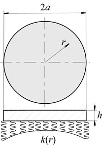
Annular (Fig. 1) and solid circular (Fig. 2) homogeneous plates with uniform flexural rigidity $D$ resting on a heterogeneous continuous Winkler elastic foundation are considered, where: $a$ – plate outer contour circle radius; $b$ – plate inner contour circle radius; $h$ – plate thickness; $r$ – radial coordinate $(0 \leq r \leq a)$ .

Fig. 1Annular plate

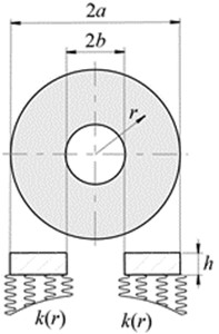
Fig. 2Solid circular plate

The plate flexural rigidity is determined using the standard expression:

D = \frac{E h^{3}}{12 (1 - μ^{2})},

where $E$ – material elastic modulus, $μ$ – Poisson’s ratio.

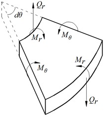
Free axisymmetric vibrations of a plate occur when the elastic foundation reaction $R (r, t)$ and the edge boundary conditions are independent of the polar angle $θ$ . Under these vibration conditions, the plate experiences only three types of dynamic internal forces (Fig. 3): $M_{r} (r, t)$ – radial bending moment; $M_{θ} (r, t)$ – as circumferential bending moment; $Q_{r} (r, t)$ – radial transverse force.

Following the Winkler hypothesis, the correlation between the foundation reaction $R (r, t)$ and the dynamic deflection of the plate $W (r, t)$ is expressed by the following equation $R (r, t) = - k (r) W (r, t)$ , where $k (r)$ – variable subgrade modulus. Relatively to $k (r)$ accept the entry form:

1

k (r) = k_{0} B (r),

where $k_{0}$ represents the subgrade modulus at a characteristic point; $B (r)$ denotes a dimensionless continuous function describing the variation of the subgrade modulus.

Fig. 3Bending moments and transverse forces in the plate

The vibration differential equation is [12], [13]:

2

D \frac{1}{r} \frac{\partial}{\partial r} \{r \frac{\partial}{\partial r} [\frac{1}{r} \frac{\partial}{\partial r} (r \frac{\partial W}{\partial r})]\} + k_{0} B (r) W + ρ h \frac{\partial^{2} W}{\partial t^{2}} = 0,

where $ρ$ – material density. Finding an exact solution to this equation is the central problem of the study.

3. General integral of the vibration equation and exact expressions for dynamic deflections and internal forces

Dynamic movements include deflection $W (r, t)$ and the angle of rotation $φ (r, t)$ . After subtracting from Eq. (2) the deflection function will be found $W (r, t)$ , dynamic angle of rotation $φ (r, t)$ and dynamic forces in the plate $M_{r} (r, t)$ , $M_{θ} (r, t)$ , $Q_{r} (r, t)$ are determined by well-known formulas [12]:

3

φ (r, t) = \frac{\partial W}{\partial r},

4

M_{r} (r, t) = - D (\frac{\partial^{2} W}{\partial r^{2}} + \frac{μ}{r} \frac{\partial W}{\partial r}),

5

M_{θ} (r, t) = - D (μ \frac{\partial^{2} W}{\partial r^{2}} + \frac{1}{r} \frac{\partial W}{\partial r}),

6

Q_{r} (r, t) = - D (\frac{\partial^{3} W}{\partial r^{3}} + \frac{1}{r} \frac{\partial^{2} W}{\partial r^{2}} - \frac{1}{r^{2}} \frac{\partial W}{\partial r}) .

Using the Fourier method, we look for the solution of Eq. (2) in the form of;

7

W (r, t) = w (r) T (t),

where $w (r)$ – deflections amplitude function that depends solely on the coordinate $r$ , $T (t)$ – is a function of time. Substituting Eq. (7) into Eq. (2) and distributing the variables, we get two ordinary differential equations:

8

\dot{T} (t) + ω^{2} T (t) = 0,

9

D \frac{1}{r} \frac{d}{\partial r} \{r \frac{d}{\partial r} [\frac{1}{r} \frac{d}{\partial r} (r \frac{d w}{\partial r})]\} + (k_{0} B (r) - ρ h ω^{2}) w = 0,

where $ω^{2}$ is the constant of the Fourier method.

The solution to the Eq. (8) is obvious:

T (t) = T (0) \cos ω t + \frac{\dot{T} (0)}{ω} \sin ω t,

where $T (0)$ , $\dot{T} (0)$ – parameters of the initial conditions of motion. It follows that the introduced constant value $ω$ is the frequency of the plate free vibration.

The principal mode of vibration is determined as the solution to Eq. (9), which can be reformulated as:

10

Δ Δ w + \frac{1}{a^{4}} (K B (r) - Ω^{2}) w = 0,

where $Δ = \frac{d^{2}}{d r^{2}} + \frac{1}{r} + \frac{d}{d r}$ – Laplace operator; $K = \frac{a^{4} k_{0}}{D}$ – established dimensionless parameter; $Ω$ – a dimensionless frequency defined in relation to the actual frequency $ω$ through the following equation:

11

Ω^{2} = \frac{a^{4} ρ h ω^{2}}{D} .

We denote as $X_{1} (r)$ , $X_{2} (r)$ , $Y_{1} (r)$ , $Y_{2} (r)$ the sought fundamental functions of the Eq. (10), and $Y_{1} (r)$ , $Y_{2} (r)$ let’s search as the representation:

12

Y_{n} (r) = X_{n} (r) \ln \frac{r}{a} + Z_{n} (r), (n = 1,2),

where $Z_{1} (r)$ , $Z_{2} (r)$ – auxiliary functions that are not yet known. By substituting Eq. (12) into Eq. (10), after the transformations we get:

13

(Δ Δ X_{n} (r) + \frac{1}{a^{4}} (K B (r) - Ω^{2}) X_{n} (r)) \ln \frac{r}{a} + Δ Δ Z_{n} (r) + \frac{1}{a^{4}} (K B (r) - Ω^{2}) Z_{n} (r) + \frac{4}{r} \frac{d^{3} X_{n} (r)}{d r^{3}} = 0 .

Since the expression at the logarithm in Eq. (13) must be exactly zero, according to the condition $X_{n} (r)$ $(n = 1,2)$ – solutions of the Eq. (10). So, instead of the Eq. (13) we can record:

14

Δ Δ X_{n} (r) + \frac{1}{a^{4}} (K B (r) - Ω^{2}) X_{n} (r) = 0, (n = 1,2),

15

Δ Δ Z_{n} (r) + \frac{1}{a^{4}} (K B (r) - Ω^{2}) Z_{n} (r) = - \frac{4}{r} \frac{d^{3} X_{n} (r)}{d r^{3}}, (n = 1,2) .

Solutions to the Eqs. (14) are sought in the format of double series:

16

X_{n} (r) = \sum_{m = 0}^{\infty} \sum_{k = 0}^{\infty} (- K)^{k} Ω^{2 m} α_{n, m, k} (r),

where $α_{n, m, k} (r) (n = 1,2)$ – sought variable coefficients, which are assumed to be continuous as well as their first- to fourth-order derivatives.

For now, it is assumed that Eq. (15) and series alike, in which instead of $α_{n, m, k} (r) (n = 1,2)$ its first- to fourth-order derivatives appear, converge uniformly. Then, it will be possible to differentiate the series.

Substituting Eq. (15) into Eq. (14), we get:

\sum_{m = 0}^{\infty} \sum_{k = 0}^{\infty} (- K)^{k} Ω^{2 m} Δ Δ α_{n, m, k} (r) - \frac{1}{a^{4}} B (r) \sum_{m = 0}^{\infty} \sum_{k = 0}^{\infty} (- K)^{k + 1} Ω^{2 m} α_{n, m, k} (r) - \frac{1}{a^{4}} \sum_{m = 0}^{\infty} \sum_{k = 0}^{\infty} (- K)^{k} Ω^{2 m + 2} α_{n, m, k} (r) = 0,

or:

\sum_{m = 0}^{\infty} \sum_{k = 0}^{\infty} (- K)^{k} Ω^{2 m} Δ Δ α_{n, m, k} (r) - \frac{1}{a^{4}} B (r) \sum_{m = 0}^{\infty} \sum_{k = 1}^{\infty} (- K)^{k} Ω^{2 m} α_{n, m, k - 1} (r) - \frac{1}{a^{4}} \sum_{m = 1}^{\infty} \sum_{k = 0}^{\infty} (- K)^{k} Ω^{2 m} α_{n, m - 1, k} (r) = 0 .

Then, after the transformations, we come to the need to fulfill the identity:

Δ Δ α_{n, 0,0} (r) + \sum_{k = 1}^{\infty} (- K)^{k} (Δ Δ α_{n, 0, k} (r) - \frac{1}{a^{4}} B (r) α_{n, 0, k - 1} (r)) + \sum_{m = 1}^{\infty} Ω^{2 m} (Δ Δ α_{n, m, 0} (r) - \frac{1}{a^{4}} α_{n, m - 1,0} (r)) + \sum_{m = 1}^{\infty} \sum_{k = 1}^{\infty} (- K)^{k} Ω^{2 m} (Δ Δ α_{n, m, k} (r) - \frac{1}{a^{4}} B (r) α_{n, m, k - 1} (r) - \frac{1}{a^{4}} α_{n, m - 1, k} (r)) = 0 .

To satisfy this identity, we equate all the variable coefficients at the powers to zero $(- K)^{k} Ω^{2 m}$ . Then, we transition from the operator to the explicit form of writing. As a result, we get the differential equations:

17

\frac{1}{r} \frac{d}{d r} \{r \frac{d}{d r} [\frac{1}{r} \frac{d}{d r} (r \frac{d α_{n, 0,0} (r)}{d r})]\} = 0, (n = 1,2),

18

\frac{1}{r} \frac{d}{d r} \{r \frac{d}{d r} [\frac{1}{r} \frac{d}{d r} (r \frac{d α_{n, m, 0} (r)}{d r})]\} = \frac{1}{a^{4}} α_{n, m - 1,0} (r), (m = 1,2, 3, . . .),

19

\frac{1}{r} \frac{d}{d r} \{r \frac{d}{d r} [\frac{1}{r} \frac{d}{d r} (r \frac{d α_{n, 0, k} (r)}{d r})]\} = \frac{1}{a^{4}} B (r) α_{n, 0, k - 1} (r), (k = 1,2, 3, . . .),

20

\frac{1}{r} \frac{d}{d r} \{r \frac{d}{d r} [\frac{1}{r} \frac{d}{d r} (r \frac{d α_{n, m, k} (r)}{d r})]\} = \frac{1}{a^{4}} B (r) α_{n, m, k - 1} (r) + \frac{1}{a^{4}} α_{n, m - 1, k} (r),

(m = 1,2, 3, . . .), (k = 1,2, 3, . . .) .

As $α_{1,0, 0} (r), α_{2,0, 0} (r)$ select the next functions:

21

α_{1,0, 0} (r) = 1, α_{2,0, 0} (r) = {(\frac{r}{a})}^{2} .

Obviously, each of them satisfies the Eq. (17). Next, integrating Eq. (18-20) and presuming integration constants are equal to zero, we get:

22

α_{n, m, 0} (r) = \frac{1}{a^{4}} \int_{0}^{r} \frac{1}{r} \int_{0}^{r} r \int_{0}^{r} \frac{1}{r} \int_{0}^{r} r α_{n, m - 1,0} (r) d r d r d r d r, (m = 1,2, 3, . . .),

23

α_{n, 0, k} (r) = \frac{1}{a^{4}} \int_{0}^{r} \frac{1}{r} \int_{0}^{r} r \int_{0}^{r} \frac{1}{r} \int_{0}^{r} r B (r) α_{n, 0, k - 1} (r) d r d r d r d r, (k = 1,2, 3, . . .),

24

α_{n, m, k} (r) = \frac{1}{a^{4}} \int_{0}^{r} \frac{1}{r} \int_{0}^{r} r \int_{0}^{r} \frac{1}{r} \int_{0}^{r} r (B (r) α_{n, m, k - 1} (r) + α_{n, m - 1, k} (r)) d r d r d r d r,

(m = 1,2, 3, . . .), (k = 1,2, 3, . . .) .

As can be seen, formulas Eq. (22-24) are recursive. Using these formulas, $α_{1, m, 0} (r)$ , $α_{2, m, 0} (r)$ , $α_{1,0, k} (r)$ , $α_{2,0, k} (r)$ , $α_{1, m, k} (r)$ , $α_{2, m, k} (r)$ , which will be named as generating [15], [31], [32], are sequentially determined from the known primary $α_{n, 0,0} (r)$ . For found variable coefficients of the series Eq. (16), the Eq. (14) are satisfied identically.

Let us now turn to the Eq. (15). As you can see, they are similar to the Eq. (14). The only difference is that the Eq. (15) are inhomogeneous. Accordingly, by employing the same method as in the previous case, we derive the solutions to Eq. (15). Leaving out details, only the final formulas that define the desired solutions will be presented:

25

Z_{n} (r) = \sum_{m = 0}^{\infty} \sum_{k = 0}^{\infty} (- K)^{k} Ω^{2 m} β_{n, m, k} (r),

26

β_{n, 0,0} (r) = α_{n, 0,0} (r) = {(\frac{r}{a})}^{2 n - 2}, (n = 1,2),

27

β_{n, m, 0} (r) = \frac{1}{a^{4}} \int_{0}^{r} \frac{1}{r} \int_{0}^{r} r \int_{0}^{r} \frac{1}{r} \int_{0}^{r} (r β_{n, m - 1,0} (r) - 4 a^{4} \frac{d^{3} α_{n, m, 0} (r)}{d r^{3}}) d r d r d r d r,

(m = 1,2, 3, . . .),

28

β_{n, 0, k} (r) = \frac{1}{a^{4}} \int_{0}^{r} \frac{1}{r} \int_{0}^{r} r \int_{0}^{r} \frac{1}{r} \int_{0}^{r} (r B (r) β_{n, 0, k - 1} (r) - 4 a^{4} \frac{d^{3} α_{n, 0, k} (r)}{d r^{3}}) d r d r d r d r,

(k = 1,2, 3, . . .)

29

β_{n, m, k} (r) = \frac{1}{a^{4}} \int_{0}^{r} \frac{1}{r} \int_{0}^{r} r \int_{0}^{r} \frac{1}{r} \int_{0}^{r} (r B (r) β_{n, m, k - 1} (r) + β_{n, m - 1, k} (r) - 4 a^{4} \frac{d^{3} α_{n, m, k} (r)}{d r^{3}}) d r d r d r d r, (m = 1,2, 3, . . .), (k = 1,2, 3, . . .) .

Rows Eq. (16), (25) coincide evenly. Here is a proof of convergence, for example, for the series Eq. (16). First of all, let us note that the generating functions $α_{n, m, 0} (r) (m = 1,2, 3, . . .)$ are calculated by the Eqs. (21), (22) explicitly:

30

α_{n, m, 0} (r) = c_{n, m, 0,0} {(\frac{r}{a})}^{2 n + 4 m - 2}, (m = 1,2, 3, . . .),

31

c_{n, m, 0,0} = \frac{1}{(2^{2 m} (n + 2 m - 1)!)^{2}} .

For other productive functions, denoting $γ = \underset{0 \leq r \leq a}{m a x} B (r)$ and by applying integral properties, we derive following estimates:

32

α_{n, 0, k} (r) \leq \frac{γ}{a^{4}} \int_{0}^{r} \frac{1}{r} \int_{0}^{r} r \int_{0}^{r} \frac{1}{r} \int_{0}^{r} r α_{n, 0, k - 1} (r) d r d r d r d r, (k = 1,2, 3, . . .),

33

α_{n, m, k} (r) \leq \frac{1}{a^{4}} \int_{0}^{r} \frac{1}{r} \int_{0}^{r} r \int_{0}^{r} \frac{1}{r} \int_{0}^{r} r (γ α_{n, m, k - 1} (r) + α_{n, m - 1, k} (r)) d r d r d r d r,

(m = 1,2, 3, . . .), (k = 1,2, 3, . . .) .

Next, performing sequential operations using recursive Eqs. (32), (33) for the specified index values $m$ , $k$ taking into account Eqs. (30), (31), in relation to the generating functions Eqs. (22-24) we come to the following general formula:

34

α_{n, m, k} (r) \leq \frac{γ^{k} C_{m + k}^{m}}{(2^{2 (m + k)} (n + 2 (m + k) - 1)!)^{2}} {(\frac{r}{a})}^{2 n + 4 (m + k) - 2},

(m = 0,1, 2, . . .), (k = 0,1, 2, . . .),

where $C_{m + k}^{m}$ – is the number of connections with $m + k$ by $m$ .

By applying Eq. (34) for series Eq. (16) we get:

|X_{n} (r)| \leq \sum_{m = 0}^{\infty} \sum_{k = 0}^{\infty} (γ K)^{k} Ω^{2 m} \frac{(m + k)!}{m! k! (2^{2 (m + k)} (n + 2 (m + k) - 1)!)^{2}} {(\frac{r}{a})}^{2 n + 4 (m + k) - 2} \leq \sum_{m = 0}^{\infty} \sum_{k = 0}^{\infty} \frac{(γ K)^{k} Ω^{2 m}}{m! k!} = \exp (γ K + Ω^{2}), (n = 1,2) .

As you can see, the constant acts as a majorant here. This proves that the series Eq. (16) converge absolutely and uniformly. Similarly, uniform convergence is proven for the other series that are formed from derivatives of $α_{n, m, k} (r)$ , $β_{n, m, k} (r) (n = 1,2)$ .

Let us now prove linear independency of the functions $X_{1} (r)$ , $X_{2} (r)$ , $Y_{1} (r)$ , $Y_{2} (r)$ by reverse method, assuming that the following is true:

35

C_{1} X_{1} (r) + C_{2} X_{2} (r) + C_{3} Y_{1} (r) + C_{4} Y_{2} (r) = 0,

provided that not all constants $C_{1}$ , $C_{2}$ , $C_{3}$ , $C_{4}$ are zero. Considering Eq. (12) and separately setting the logarithmic expression equal to zero, we get:

C_{3} X_{1} (r) + C_{4} X_{2} (r) = \sum_{m = 0}^{\infty} \sum_{k = 0}^{\infty} (- K)^{k} Ω^{2 m} (C_{3} α_{1, m, k} (r) + C_{4} α_{2, m, k} (r)) = 0 .

This equation is true for all $K$ , $Ω$ cases only if the following conditions are satisfied:

C_{3} α_{1, m, k} (r) + C_{4} α_{2, m, k} (r) = 0, (m = 0,1, 2, \dots), (k = 0,1, 2, \dots) .

In particular, when $m = 0$ , $k = 0$ , must be fulfilled $C_{3} + C_{4} {(\frac{r}{a})}^{2} = 0$ . Hence:

36

C_{3} = C_{4} = 0,

i.e. functions $X_{1} (r)$ , $X_{2} (r)$ – are linearly independent. Given this fact, as well as the Eq. (36), it follows from identity Eq. (35) that $C_{1} = C_{2} = C_{3} = C_{4} = 0$ . This proves linear independency of the system of functions $X_{1} (r)$ , $X_{2} (r)$ , $Y_{1} (r)$ , $Y_{2} (r)$ .

As a result, it can be claimed that Eqs. (12), (16), (21-29) describe four fundamental functions $X_{1} (r)$ , $X_{2} (r)$ , $Y_{1} (r)$ , $Y_{2} (r)$ of Eq. (10). By analyzing the mentioned formulas, we conclude that the functions $X_{1} (r)$ , $X_{2} (r)$ , $Z_{1} (r)$ , $Z_{2} (r)$ are dimensionless [15]. For this reason, the functions $Y_{1} (r)$ , $Y_{2} (r)$ are also dimensionless.

Therefore, the general solution of Eq. (10) is expressed as:

37

w (r) = C_{1} X_{1} (r) + C_{2} X_{2} (r) + C_{3} Y_{1} (r) + C_{4} Y_{2} (r),

where $C_{1}$ , $C_{2}$ , $C_{3}$ , $C_{4}$ – arbitrary constants, which are of the same unit as deflection. By assuming that $C_{n} = a λ_{n} (n = 1,2)$ , where $λ_{1}$ , $λ_{2}$ – arbitrary dimensionless constants, then Eq. (37) can be expressed as:

38

w (r) = a w_{0} (r),

39

w_{0} (r) = λ_{1} X_{1} (r) + λ_{2} X_{2} (r) + λ_{3} Y_{1} (r) + λ_{4} Y_{2} (r),

where $w_{0} (r)$ is a dimensionless function. the expressions for the function $w (r)$ first three derivatives are also provided as follows:

40

\frac{d w}{d r} = {\tilde{w}}_{0} (r),

41

{\tilde{w}}_{0} (r) = λ_{1} {\tilde{X}}_{1} (r) + λ_{2} {\tilde{X}}_{2} (r) + λ_{3} {\tilde{Y}}_{1} (r) + λ_{4} {\tilde{Y}}_{2} (r),

42

\frac{d^{2} w}{d r^{2}} = \frac{1}{a} {\overset{̑}{w}}_{0} (r),

43

{\overset{̑}{w}}_{0} (r) = λ_{1} {\overset{̑}{X}}_{1} (r) + λ_{2} {\overset{̑}{X}}_{2} (r) + λ_{3} {\overset{̑}{Y}}_{1} (r) + λ_{4} {\overset{̑}{Y}}_{2} (r),

44

\frac{d^{3} w}{d r^{3}} = \frac{1}{a^{2}} {\hat{w}}_{0} (r),

45

{\hat{w}}_{0} (r) = λ_{1} {\hat{X}}_{1} (r) + λ_{2} {\hat{X}}_{2} (r) + λ_{3} {\hat{Y}}_{1} (r) + λ_{4} {\hat{Y}}_{2} (r),

where:

46

{\tilde{X}}_{n} (r) = a \frac{d X_{n} (r)}{d r}, {\overset{̑}{X}}_{n} (r) = a^{2} \frac{d^{2} X_{n} (r)}{d r^{2}}, {\hat{X}}_{n} (r) = a^{3} \frac{d^{3} X_{n} (r)}{d r^{3}}, (n = 1,2),

47

{\tilde{Y}}_{n} (r) = a \frac{d Y_{n} (r)}{d r}, {\overset{̑}{Y}}_{n} (r) = a^{2} \frac{d^{2} Y_{n} (r)}{d r^{2}}, {\hat{Y}}_{n} (r) = a^{3} \frac{d^{3} Y_{n} (r)}{d r^{3}}, (n = 1,2) .

Functions Eqs. (46), (47), unlike derivative functions $X_{n} (r)$ , $Y_{n} (r)$ , will be dimensionless [15] and will be called dimensionless derivatives from now on. In this case, taking into account Eq. (12), the dimensionless derivatives given in Eq. (47) yield:

{\tilde{Y}}_{n} (r) = {\tilde{X}}_{n} (r) \ln \frac{r}{a} + \frac{a}{r} X_{n} (r) + {\tilde{Z}}_{n} (r),

{\overset{̑}{Y}}_{n} (r) = {\overset{̑}{X}}_{n} (r) \ln \frac{r}{a} + \frac{2 a}{r} {\tilde{X}}_{n} (r) - {(\frac{a}{r})}^{2} X_{n} (r) + {\overset{̑}{Z}}_{n} (r),

{\hat{Y}}_{n} (r) = {\hat{X}}_{n} (r) \ln \frac{r}{a} + \frac{3 a}{r} {\overset{̑}{X}}_{n} (r) - 3 {(\frac{a}{r})}^{2} {\tilde{X}}_{n} (r) + 2 {(\frac{a}{r})}^{3} X_{n} (r) + {\hat{Z}}_{n} (r),

where:

{\tilde{Z}}_{n} (r) = a \frac{d Z_{n} (r)}{d r}, {\overset{̑}{Z}}_{n} (r) = a^{2} \frac{d^{2} Z_{n} (r)}{d r^{2}}, {\hat{Z}}_{n} (r) = a^{3} \frac{d^{3} Z_{n} (r)}{d r^{3}},

are dimensionless derivatives of functions $Z_{1} (r)$ , $Z_{2} (r)$ .

Therefore, the amplitude function of deflection and its first three derivatives are expressed in terms of dimensionless functions $w_{0} (r)$ , ${\tilde{w}}_{0} (r)$ , ${\overset{̑}{w}}_{0} (r)$ , ${\hat{w}}_{0} (r)$ . Consequently, the formulations for dynamic deflections Eq. (3), (7), as well as for dynamic internal forces Eqs. (4-6), when accounting for Eqs. (38), (40), (42), (44), take the following form:

48

W (r, t) = a w_{0} (r) T (t),

49

φ (r, t) = {\tilde{w}}_{0} (r) T (t),

50

M_{r} (r, t) = - \frac{D}{a} ({\overset{̑}{w}}_{0} (r) + μ \frac{a}{r} {\tilde{w}}_{0} (r)) T (t),

51

M_{θ} (r, t) = - \frac{D}{a} (μ {\overset{̑}{w}}_{0} (r) + \frac{a}{r} {\tilde{w}}_{0} (r)) T (t),

52

Q_{r} (r, t) = - \frac{D}{a^{2}} ({\hat{w}}_{0} (r) + \frac{a}{r} {\overset{̑}{w}}_{0} (r) - {(\frac{a}{r})}^{2} {\tilde{w}}_{0} (r)) T (t) .

Consequently, dynamic parameters were expressed in terms of dimensionless fundamental functions $X_{1} (r)$ , $X_{2} (r)$ , $Y_{1} (r)$ , $Y_{2} (r)$ and their dimensionless derivatives, enabling the use of mostly dimensionless quantities in modal analysis of plates.

4. Vibration frequency analytical representation

According to Eq. (11), we obtain the frequency spectrum:

53

ω_{j} = \frac{Ω_{j}}{a^{2}} \sqrt{\frac{D}{ρ h}}, (j = 1,2, 3, \dots),

where $Ω_{j}$ are positive roots of the frequency Eq. (37) sorted in ascending order. Essentially, determining the frequency $ω$ reduces to evaluating the corresponding dimensionless frequency $Ω$ . Since the fundamental functions $X_{1} (r)$ , $X_{2} (r)$ and their dimensionless derivatives depend on the dimensionless frequency, then the frequency equations obtained after the implementation of the specified boundary conditions will serve to find it.

5. Representation of product functions by power series

For the study of free vibrations of circular plates, the exact formulas were obtained Eqs. (38-45), (48)-(52). However, the practical implementation of these formulas requires repeated calculation of integrals Eq. (22-24), (27-29), which define the generating functions. However, such calculations can be difficult, which, in turn, can be an obstacle to the application of the results in engineering practice. Therefore, for the convenience of numerical realization, we will write the product functions in the form of power series.

As can be seen from the Eq. (30), generating functions $α_{n, m, 0} (r) (m = 1,2, 3, . . .)$ are already polynomials (finite power series). In the subsequent analysis, we consider the dimensionless continuous function $B (r)$ is regular near $r = 0$ and expressed by the Maclaurin series:

54

B (r) = B_{0} + B_{1} (\frac{r}{a}) + B_{2} {(\frac{r}{a})}^{2} + . . . + B_{j} {(\frac{r}{a})}^{j} + . . .,

where:

B_{0} = B (0), B_{j} = \frac{a^{j} B^{(j)} (0)}{j!}, (j = 1,2, 3, . . .),

are dimensionless coefficients, and the index $(j)$ denotes the order of the derivative. From Eqs. (23), (21), (54) it is evident that the generating functions $α_{n, 0, k} (r) (k = 1,2, 3, . . .)$ are likewise expressed as power series, with their lowest power equal to $2 n + 4 k - 2$ . Hence, functions $α_{1,0, k} (r)$ , $α_{2,0, k} (r) (k = 1,2, 3, . . .)$ can be written in the form:

55

α_{n, 0, k} (r) = {(\frac{r}{a})}^{2 n + 4 k - 2} \sum_{j = 0}^{\infty} c_{n, 0, k, j} {(\frac{r}{a})}^{j}, (k = 1,2, 3, . . .),

where $c_{n, 0, k, j}$ – dimensionless coefficients to be determined. At the same time, in a particular case $k = 0$ Eq. (55) must coincide with Eq. (21). From this condition we find:

56

c_{n, 0,0, 0} = 1, c_{n, 0,0, j} = 0, (j = 1,2, 3, . . .) .

Using the form of Eq. (54), as well as equation:

α_{n, 0, k - 1} (r) = {(\frac{r}{a})}^{2 n + 4 k - 6} \sum_{j = 0}^{\infty} c_{n, 0, k - 1, j} {(\frac{r}{a})}^{j},

which is a consequence of Eq. (55), find the product of the series:

57

B (r) α_{n, 0, k - 1} (r) = {(\frac{r}{a})}^{2 n + 4 k - 6} {\sum_{j = 0}^{\infty} e_{n, 0, k - 1, j} (\frac{r}{a})}^{j},

where:

58

e_{n, 0, k - 1, j} = \sum_{i = 0}^{j} B_{j - i} c_{n, 0, k - 1, i} .

Substituting the value of Eq. (57) into Eq. (23) in place of the product $B (r) α_{n, 0, k - 1} (r)$ and carrying out the integration, yields the following result:

59

α_{n, 0, k} (r) = {(\frac{r}{a})}^{2 n + 4 k - 2} \sum_{j = 0}^{\infty} \frac{e_{n, 0, k - 1, j}}{p_{n, 0, k, j}^{2}} {(\frac{r}{a})}^{j},

where $p_{n, 0, k, j} = (2 n + 4 k + j - 4) (2 n + 4 k + j - 2)$ .

By comparing Eq. (55) and (59), and factoring in Eq. (58), the following recursive formula for the coefficients of interest is obtained:

60

c_{n, 0, k, j} = \frac{1}{p_{n, 0, k, j}^{2}} \sum_{i = 0}^{j} B_{j - i} c_{n, 0, k - 1, i}, (k = 1,2, 3, . . .), (j = 0,1, 2, . . .) .

So, Eqs. (56), (60) fully define series coefficients Eq. (55).

Analyzing the Eq. (24) taking into account Eqs. (30), (54), (55), we come to the conclusion that the generating functions $α_{n, m, k} (r)$ will also be power series with the lowest power of $2 n + 4 (m + k) - 2$ . Accordingly, the expression can be written as:

61

α_{n, m, k} (r) = {(\frac{r}{a})}^{2 n + 4 (m + k) - 2} \sum_{j = 0}^{\infty} c_{n, m, k, j} {(\frac{r}{a})}^{j}, (m = 1,2, 3, . . .), (k = 1,2, 3, . . .),

where $c_{n, m, k, j}$ – the desired dimensionless coefficients. The case of $k = 0$ requires separate consideration. In this case, the Eq. (61) must coincide with Eq. (30), what will be ensured if:

62

c_{n, m, 0, j} = 0, (m = 1,2, 3, . . .), (j = 1,2, 3, . . .) .

By shifting indices $m$ and $k$ in Eq. (61) by one at a time, we get:

63

α_{n, m - 1, k} (r) = {(\frac{r}{a})}^{2 n + 4 (m + k) - 6} \sum_{j = 0}^{\infty} c_{n, m - 1, k, j} {(\frac{r}{a})}^{j},

64

α_{n, m, k - 1} (r) = {(\frac{r}{a})}^{2 n + 4 (m + k) - 6} \sum_{j = 0}^{\infty} c_{n, m, k - 1, j} {(\frac{r}{a})}^{j} .

As the product of the series Eqs. (54) and (64) we get

65

B (r) α_{n, m, k - 1} (r) = {(\frac{r}{a})}^{2 n + 4 (m + k) - 6} {\sum_{j = 0}^{\infty} e_{n, m, k - 1, j} (\frac{r}{a})}^{j},

where:

66

e_{n, m, k - 1, j} = \sum_{i = 0}^{j} B_{j - i} c_{n, m, k - 1, i} .

By substituting the values of Eqs. (63), (65) into Eq. (24) replacing the expressions $B (r) α_{1, m, k - 1} (r)$ , $B (r) α_{2, m, k - 1} (r)$ , $α_{1, m - 1, k} (r)$ , $α_{2, m - 1, k} (r)$ and subsequently performing the integration, we obtain:

67

α_{n, m, k} (r) = {(\frac{r}{a})}^{2 n + 4 (m + k) - 2} \sum_{j = 0}^{\infty} \frac{e_{n, m, k - 1, j} + c_{n, m - 1, k, j}}{p_{n, m, k, j}^{2}} {(\frac{r}{a})}^{j},

(m = 1,2, 3, . . .), (k = 1,2, 3, . . .),

where $p_{n, m, k, j} = (2 n + 4 (m + k) + j - 4) (2 n + 4 (m + k) + j - 2)$ .

Comparing Eqs. (61) and (67), and factoring in Eq. (66), we derive the following recursive relation for the coefficients of interest:

68

c_{n, m, k, j} = \frac{1}{p_{n, m, k, j}^{2}} (c_{n, m - 1, k, j} + \sum_{i = 0}^{j} B_{j - i} c_{n, m, k - 1, i}),

(m = 1,2, 3, . . .), (k = 1,2, 3, . . .), (j = 0,1, 2, . . .) .

Thus, the recursive Eqs. (31), (60), (62), (68) fully define the dimensionless coefficients of Eq. (61).

Similarly, you can get a representation in the form of power series for generating functions Eqs. (27)-(29). Here are given only the final formulas:

69

β_{n, m, 0} (r) = d_{n, m, 0,0} {(\frac{r}{a})}^{2 n + 4 m - 2}, (m = 1,2, 3, . . .),

70

d_{n, 0,0, 0} = 1, d_{n, m, 0,0} = \frac{d_{n, m - 1,0, 0}}{p_{n, m, 0,0}^{2}} - 4 (2 n + 4 m - 3) \frac{c_{n, m, 0,0}}{p_{n, m, 0,0}}, (m = 1,2, 3, . . .),

71

β_{n, 0, k} (r) = {(\frac{r}{a})}^{2 n + 4 k - 2} \sum_{j = 0}^{\infty} d_{n, 0, k, j} {(\frac{r}{a})}^{j},

72

d_{n, 0,0, j} = 0, (j = 1,2, 3, . . .),

73

d_{n, 0, k, j} = \frac{1}{p_{n, 0, k, j}^{2}} \sum_{i = 0}^{j} B_{j - i} d_{n, 0, k - 1, i} - 4 (2 n + 4 k + j - 3) \frac{c_{n, 0, k, j}}{p_{n, 0, k, j}},

(k = 1,2, 3, . . .), (j = 0,1, 2, . . .),

74

β_{n, m, k} (r) = {(\frac{r}{a})}^{2 n + 4 (m + k) - 2} \sum_{j = 0}^{\infty} d_{n, m, k, j} {(\frac{r}{a})}^{j}, (m = 1,2, 3, . . .), (k = 1,2, 3, . . .),

75

d_{n, m, 0, j} = 0, (m = 1,2, 3, . . .), (j = 1,2, 3, . . .),

76

d_{n, m, k, j} = \frac{1}{p_{n, m, k, j}^{2}} (d_{n, m - 1, k, j} + \sum_{i = 0}^{j} B_{j - i} d_{n, m, k - 1, i}) - 4 (2 n + 4 (m + k) + j - 3) \frac{c_{n, m, k, j}}{p_{n, m, k, j}},

(m = 1,2, 3, . . .), (k = 1,2, 3, . . .), (j = 0,1, 2, . . .) .

The set of recurrence relations Eqs. (70), (72), (73), (75), (76) completely determines the coefficients of series Eq. (74).

Eqs. (39), (41), (43) and (45) provide a general framework for analyzing the vibrations of both solid and annular plates. For solid plates, however, these equations can be further simplified. Specifically, applying the condition of finite deflection at the plate center $r = 0$ to Eq. (39) yields a reduction in the complexity of the solution $λ_{3} = λ_{4} = 0 .$ In this scenario, the fundamental functions $Y_{1} (r)$ , $Y_{2} (r)$ appearing in Eqs. (69)-(76) are not involved in the calculations.

It should also be noted that, for plates with non-smooth $B (r)$ , the problem can be addressed in a piecewise manner by discretizing the structure.

Consequently, all generating functions can be expressed as power series. Hence, an analytical method of numerical realization for the found exact solutions is actually proposed.

6. Illustrative examples

6.1. Example 1. Annular plate

Consider the scenario in which the subgrade modulus varies following a parabolic distribution:

k (r) = \frac{4 \frac{b}{a}}{{(1 - \frac{b}{a})}^{2}} k (\frac{a + b}{2}) (\frac{r}{b} - 1) (1 - \frac{r}{a}) .

Such a form of dependence is appropriate in cases where the foundation stiffness function exhibits an extremum (minimum or maximum) within the intermediate region of the annulus – for example, in the presence of a local zone of reinforcement or weakening of the foundation.

Let’s write this formula in the Eq. (1):

k (r) = k_{0} (\frac{r}{b} - 1) (1 - \frac{r}{a}), k_{0} = \frac{4 \frac{b}{a}}{{(1 - \frac{b}{a})}^{2}} k (\frac{a + b}{2}), B (r) = (\frac{r}{b} - 1) (1 - \frac{r}{a}),

i.e.:

B_{0} = - 1, B_{1} = 1 + \frac{a}{b}, B_{2} = - \frac{a}{b}, B_{j} = 0, (j = 3,4, 5, . . .) .

Here are the calculation results for annular concrete plate with clamped contours. This case corresponds to the boundary conditions: $W (a, t) = 0$ ; $φ (a, t) = 0$ ; $W (b, t) = 0$ ; $φ (b, t) = 0$ . By implementing them, using Eqs. (48), (49), (39), we have a homogeneous linear system of four equations regarding $λ_{1}$ , $λ_{2}$ , $λ_{3}$ , $λ_{4}$ . By formulating the condition for the existence of solutions to this system, we obtain the corresponding frequency equation:

77

Δ (Ω) = |\begin{matrix} X_{1} (a) & X_{2} (a) & Y_{1} (a) & Y_{2} (a) \\ {\tilde{X}}_{1} (a) & {\tilde{X}}_{2} (a) & {\tilde{Y}}_{1} (a) & {\tilde{Y}}_{2} (a) \\ X_{1} (b) & X_{2} (b) & Y_{1} (b) & Y_{2} (b) \\ {\tilde{X}}_{1} (b) & {\tilde{X}}_{2} (b) & {\tilde{Y}}_{1} (b) & {\tilde{Y}}_{2} (b) \end{matrix}| = 0 .

Once the solutions $Ω_{j} (j = 1,2, 3, \dots)$ of this equation are obtained, the natural frequencies of free axisymmetric vibrations of the plate can be determined using Eq. (53).

Input data for the calculation: $ρ =$ 2500 kg/m³; $E =$ 15 MPa; $μ =$ 1/6; $a =$ 2.5 m; $b =$ 1.5 m; $h =$ 0.12 m; $k (\frac{a + b}{2}) =$ 4×10³ kN/m³.

Table 1 summarizes the computed values for the first three vibration modes, determined using the proposed authors’ method (AM), and compares them with results obtained via the approximate finite element method (FEM) executed in the LIRA-FEM software (7560 rectangular elements). The corresponding mode shapes for these three vibration modes are illustrated in Fig. 4.

Table 1Obtained results

Mode no.	Vibration frequencies $ω$ , rad/s		Relative error, %
Mode no.	AM	FEM	Relative error, %
1	614.790850	630.461487	2.55
2	1694.701320	1736.626465	2.27
3	3328.775677	3405.004639	2.29

Fig. 4First three normalized axisymmetric vibration modes of annular plate with clamped edges

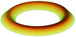
a) 1st mode

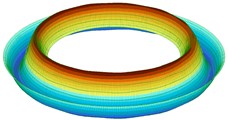
b) 2nd mode

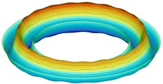
c) 3rd mode

It is important to emphasize that, in the present example, series Eq. (54) degenerates into a finite first-degree polynomial. Consequently, truncation of the series is unnecessary, and the resulting computations can be considered exact.

6.2. Example 2. Solid circular plate

Consider the scenario in which the subgrade modulus varies following an exponential distribution:

k (r) = k (0) \exp (δ \frac{r}{a}), δ = \ln \frac{k (a)}{k (0)} .

The proposed model adequately captures the gradient heterogeneity of the foundation caused by the spatial variation of its physico-mechanical properties. Variation of the model parameter enables the representation of both smooth and abrupt changes in foundation characteristics and is applicable to modeling gradual stiffness variations that cannot be accurately approximated by polynomial functions, as well as to describing transitions between more and less compacted regions or zones of reinforcement and weakening within the foundation.

The formula can be expressed in the form of Eq. (1). Specifically, if $k (0) \neq 0$ , then:

k_{0} = k (0), B (r) = \exp (δ \frac{r}{a}),

i.e.:

B_{0} = 1, B_{j} = \frac{δ^{j}}{j!}, (j = 1,2, 3, . . .) .

The computation results for a solid steel plate constrained along its edges are summarized as follows. This case corresponds to the boundary conditions: $W (a, t) = 0$ ; $φ (a, t) = 0$ . By implementing them, using Eqs. (48), (49), (39), (41), we have a homogeneous linear system of two equations regarding $λ_{1}$ , $λ_{2}$ . By formulating the condition for the existence of solutions to this system, we obtain the corresponding frequency equation:

Δ (Ω) = |\begin{matrix} X_{1} (a) & X_{2} (a) \\ {\tilde{X}}_{1} (a) & {\tilde{X}}_{2} (a) \end{matrix}| = 0 .

Once the solutions $Ω_{j} (j = 1,2, 3, \dots)$ of this equation are obtained, the natural frequencies of free axisymmetric vibrations of the plate can be determined using Eq. (53).

Input data for the calculation: $ρ =$ 7800 kg/m³; $E =$ 200 GPa; $μ =$ 0.3; $a =$ 1 m; $h =$ 0.05 m; $k (0) =$ 5×10³ kN/m³; $k (a) =$ 4×10³ kN/m³.

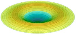
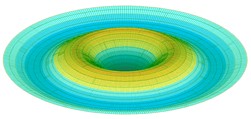
Table 2 summarizes the computed values for the first three vibration modes, determined using the proposed authors’ method (AM), and compares them with results obtained via the approximate finite element method (FEM) executed in the LIRA-FEM software (360 triangle elements in the center of the plate, 6840 rectangular elements). The corresponding mode shapes for these three vibration modes are illustrated in Fig. 5.

Table 2Obtained results

Mode No.	Vibration frequencies $ω$ , rad/s		Relative error, %
Mode No.	AM	FEM	Relative error, %
1	252.382020	256.028412	1.44
2	973.790567	996.033997	2.28
3	2180.611868	2229.999023	2.26

Fig. 5First three normalized axisymmetric vibration modes of solid circular plate with clamped edge

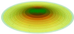
a) 1st mode

b) 2nd mode

c) 3rd mode

It should be noted that the method allows for achieving any preassigned level of computational accuracy. In particular, in the examples considered, the calculations were carried out with a precision of up to six decimal places. For the frequency values, this level of accuracy is attained by retaining the first $m = k =$ 17 terms of the series in the first example and $m = k =$ 10 terms in the second.

7. Conclusions

1) This study presents an analytical method for performing axisymmetric modal analysis of circular plates resting on a variable elastic foundation. This method eliminates the need for structural discretization and offers a robust alternative to conventional approximate techniques for addressing this class of problems.

2) As modal analysis is based on the exact solution of the governing differential equation, the obtained numerical results can be regarded as accurate. Such exact solutions serve as important reference benchmarks for evaluating the accuracy of different approximate techniques. The introduction of such methods into engineering practice will ensure greater accuracy of calculations.

3) The comparison between the AM results and the corresponding FEM results obtained using the LIRA-FEM software demonstrates the accuracy and applicability of the proposed method for the case under study.

References

Z. R. Wani et al., “A critical review on control strategies for structural vibration control,” Annual Reviews in Control, Vol. 54, pp. 103–124, 2022, https://doi.org/10.1016/j.arcontrol.2022.09.002

Publisher
N. B. Dharmajan and M. Alhamaydeh, “State-of-the-art review of structural vibration control: overview and research gaps,” Applied Sciences, Vol. 15, No. 14, p. 7966, Jul. 2025, https://doi.org/10.3390/app15147966

Publisher
X. Sun, S. Ilanko, Y. Mochida, and R. C. Tighe, “A review on vibration-based damage detection methods for civil structures,” Vibration, Vol. 6, No. 4, pp. 843–875, Oct. 2023, https://doi.org/10.3390/vibration6040051

Publisher
S. S. Saidin, A. Jamadin, S. Abdul Kudus, N. Mohd Amin, and M. A. Anuar, “An overview: the application of vibration-based techniques in bridge structural health monitoring,” International Journal of Concrete Structures and Materials, Vol. 16, No. 1, Dec. 2022, https://doi.org/10.1186/s40069-022-00557-1

Publisher
G. Wang and J. Ke, “Literature review on the structural health monitoring (SHM) of sustainable civil infrastructure: an analysis of influencing factors in the implementation,” Buildings, Vol. 14, No. 2, p. 402, Feb. 2024, https://doi.org/10.3390/buildings14020402

Publisher
H. Sun, X. Liu, B. Huang, W. Li, Y. Fang, and Y. Wang, “Improved mode decomposition method for vibration signal denoising of aero-engine shaft bearing,” Mechanical Systems and Signal Processing, Vol. 238, p. 113201, Sep. 2025, https://doi.org/10.1016/j.ymssp.2025.113201

Publisher
X. Yu, X. Liu, X. Wang, X. Wang, and Y. Wang, “Vibration control of improved LQG for wheel drive electric vehicle based on uncertain parameters,” Proceedings of the Institution of Mechanical Engineers, Part D: Journal of Automobile Engineering, Vol. 235, No. 8, pp. 2253–2264, Jan. 2021, https://doi.org/10.1177/0954407020983150

Publisher
X. T. Liu and S. S. Rao, “Vibration analysis in the presence of uncertainties using universal grey system theory,” Journal of Vibration and Acoustics, Vol. 140, No. 3, 2018, https://doi.org/10.1115/1.4038940

Publisher
Y. Wang et al., “Structural vibration monitoring with diffractive optical processors,” Science Advances, Vol. 12, No. 10, Mar. 2026, https://doi.org/10.1126/sciadv.aea1712

Publisher
O. Avci, O. Abdeljaber, S. Kiranyaz, M. Hussein, M. Gabbouj, and D. J. Inman, “A review of vibration-based damage detection in civil structures: from traditional methods to machine learning and deep learning applications,” Mechanical Systems and Signal Processing, Vol. 147, p. 107077, Jan. 2021, https://doi.org/10.1016/j.ymssp.2020.107077

Publisher
M. A. Foyouzat, M. Mofid, and J. E. Akin, “Free vibration of thin circular plates resting on an elastic foundation with a variable modulus,” Journal of Engineering Mechanics, Vol. 142, No. 4, Apr. 2016, https://doi.org/10.1061/(asce)em.1943-7889.0001050

Publisher
S. Timoshenko and S. Woinowsky-Krieger, Theory of Plates and Shells. New York, USA: McGraw-Hill, 1959.

Search CrossRef
S. Timoshenko, Vibration Problems in Engineering. New York, USA: Van Nostrand, 1955.

Search CrossRef
D. V. Vainberh and Y. D. Vainberh, Rozrakhunok Plastyn. (in Ukrainian), Kyiv, Ukraine: Budivelnyk, 1970.

Search CrossRef
Y. S. Krutii, M. G. Sur’Yaninov, and G. S. Karnaukhova, “Calculation method for axisymmetric bending of circular and annular plates on a changeable elastic bed. Part 1. Analytical relations,” Strength of Materials, Vol. 53, No. 2, pp. 247–257, Jul. 2021, https://doi.org/10.1007/s11223-021-00282-2

Publisher
Y. S. Krutii, M. G. Sur’Yaninov, M. M. Soroka, and G. S. Karnaukhova, “Calculation method for axisymmetric bending of circular and annular plates on a changeable elastic bed. Part 2. Calculation results for continuous circular plates,” Strength of Materials, Vol. 53, No. 3, pp. 417–422, Oct. 2021, https://doi.org/10.1007/s11223-021-00301-2

Publisher
P. A. A. Laura, R. H. Gutierrez, R. Carnicer, and H. C. Sanzi, “Free vibrations of a solid circular plate of linearly varying thickness and attached to a Winkler foundation,” Journal of Sound and Vibration, Vol. 144, No. 1, pp. 149–161, Jan. 1991, https://doi.org/10.1016/0022-460x(91)90738-6

Publisher
Z. C. Girgin and K. Girgin, “A numerical method for static or dynamic stiffness matrix of non-uniform members resting on variable elastic foundations,” Engineering Structures, Vol. 27, No. 9, pp. 1373–1384, Aug. 2005, https://doi.org/10.1016/j.engstruct.2005.04.005

Publisher
S. M. Mirkhalaf Valashani, “Transverse vibration of clamped and simply supported circular plates with an eccentric circular perforation and attached concentrated mass,” Journal of Solid Mechanics, Vol. 1, No. 1, pp. 37–44, 2009.

Search CrossRef
C. K. Rao and L. B. Rao, “Vibrations of elastically restrained circular plates resting on partial Winkler foundation,” The Open Acoustics Journal, Vol. 2, No. 1, pp. 68–74, 2009, https://doi.org/10.2174/1874837600902010068

Publisher
J. H. Haido, B. H. A. Bakar, A. A. Abdul-Razzak, and J. Jayaprakash, “Dynamic performance of circular reinforced concrete slabs,” in Gaza Conference, 2010.

Publisher
M. M. Alipour, M. Shariyat, and M. Shaban, “A semi-analytical solution for free vibration and modal stress analyses of circular plates resting on two-parameter elastic foundations,” Journal of Solid Mechanics, Vol. 2, No. 1, pp. 63–78, 2010, https://doi.org/10.1007/s00419-010-0484-x

Publisher
L. B. Rao and L. B. Rao, “Free vibration of circular plates with elastic edge support and resting on an elastic foundation,” The International Journal of Acoustics and Vibration, Vol. 17, No. 4, pp. 204–207, 2012, https://doi.org/10.20855/ijav.2012.17.4311

Publisher
L. B. Rao and C. K. Rao, “Vibrations of circular plates with guided edge and resting on elastic foundation,” Journal of Sound and Vibration, Vol. 331, No. 24, pp. 5300–5315, 2012.

Search CrossRef
M. Tufoi et al., “An analysis of the dynamic behavior of circular plates from a damage detection perspective,” Romanian Journal of Acoustics and Vibration, Vol. 11, No. 1, pp. 41–46, 2014.

Search CrossRef
L. B. Rao and C. K. Rao, “Vibrations of circular plates resting on elastic foundation with elastically restrained edge against translation,” The Journal of Engineering Research [TJER], Vol. 13, No. 1, pp. 14–25, 2018, https://doi.org/10.24200/tjer.vol15iss1pp14-25

Publisher
S. A. Salawu, M. G. Sobamowo, and O. M. Sadiq, “Analytical approach into dynamic behavior of functionally graded circular plates resting on two-parameter foundations under excitation force,” The Scientific World Journal, Vol. 139, No. 2, pp. 115–134, 2019.

Search CrossRef
S. A. Salawu, M. G. Sobamowo, and O. M. Sadiq, “Dynamic investigation of nonlinear free vibration of circular plates resting on Winkler and Pasternak foundations,” International Journal of Mechanical Handling and Automation, Vol. 5, No. 2, pp. 19–42, 2019.

Search CrossRef
S. A. Salawu, G. M. Sobamowo, and O. M. Sadiq, “Investigation of dynamic behaviour of circular plates resting on Winkler and Pasternak foundations,” SN Applied Sciences, Vol. 1, No. 12, pp. 125–136, Dec. 2019, https://doi.org/10.1007/s42452-019-1588-8

Publisher
M. G. Sobamowo and S. A. Salawu, “Free vibration analysis of nonlinear circular plates resting on Winkler and Pasternak foundations,” Journal of Solid Mechanics, Vol. 12, No. 1, pp. 121–135, 2020.

Publisher
Y. Krutii, A. Perperi, S. Nikipchuk, I. Butrynskyi, and D. Velychko, “Modal analysis of circular plates resting on an inhomogeneous elastic Winkler foundation,” Vibroengineering Procedia, Vol. 59, pp. 133–138, Sep. 2025, https://doi.org/10.21595/vp.2025.25282

Publisher
Y. Krutii, M. Suriyaninov, and V. Vandynskyi, “Analytic formulas for the natural frequencies of hinged structures with taking into account the dead weight,” MATEC Web of Conferences, Vol. 230, p. 02016, 2018, https://doi.org/10.1051/matecconf/201823002016

Publisher

About this article

Received

January 17, 2026

Accepted

April 7, 2026

Published

June 30, 2026

DOI

https://doi.org/10.21595/mme.2026.26028

Keywords

circular plate

inhomogeneous foundation

Winkler’s hypothesis

variable subgrade modulus

analytical calculation method

modal analysis

Acknowledgements

The authors have not disclosed any funding.

Data Availability

The datasets generated during and/or analyzed during the current study are available from the corresponding author on reasonable request.

Author Contributions

Yurii Krutii: conceptualization, methodology. Alla Perperi: project administration, visualization. Roman Kachmar: formal analysis. Rostyslav Predko: writing-review and editing. Danylo Velychko: software, validation.

Conflict of interest

The authors declare that they have no conflict of interest.

This is an open access article distributed under the Creative Commons Attribution License, which permits unrestricted use, distribution, and reproduction in any medium, provided the original work is properly cited.

Previous article in issue Previous

Y. Krutii, A. Perperi, R. Kachmar, R. Predko, and D. Velychko, “Analytical method for studying free vibrations of round plates on a non-homogeneous elastic foundation,” Mathematical Models in Engineering, Vol. 12, No. 2, pp. 202–219, Jun. 2026, https://doi.org/10.21595/mme.2026.26028

Copy Extrica

Copied to clipboard!

TY  - JOUR
DO  - 10.21595/mme.2026.26028
UR  - https://doi.org/10.21595/mme.2026.26028
TI  - Analytical method for studying free vibrations of round plates on a non-homogeneous elastic foundation
T2  - Mathematical Models in Engineering
AU  - Krutii, Yurii
AU  - Perperi, Alla
AU  - Kachmar, Roman
AU  - Predko, Rostyslav
AU  - Velychko, Danylo
PY  - 2026
DA  - 2026/06/30
PB  - Extrica
SP  - 202-219
VL  - 12
IS  - 2
SN  - 2351-5279
SN  - 2424-4627
ER  - 

Copy Ris

Copied to clipboard!

@article{doi_10.21595/mme.2026.26028,
  title = {Analytical method for studying free vibrations of round plates on a non-homogeneous elastic foundation},
  author = {Krutii, Yurii and Perperi, Alla and Kachmar, Roman and Predko, Rostyslav and Velychko, Danylo},
  journal = {Mathematical Models in Engineering},
  year = {2026},
  month = {6},
  volume = {12},
  number = {2},
  pages = {202--219},
  doi = {10.21595/mme.2026.26028},
  url = {https://doi.org/10.21595/mme.2026.26028},
  publisher = {Extrica},
  issn = {2351-5279},
  eissn = {2424-4627},
}

Copy Bibtex

Copied to clipboard!

[1]Y. Krutii, A. Perperi, R. Kachmar, R. Predko, and D. Velychko, “Analytical method for studying free vibrations of round plates on a non-homogeneous elastic foundation,” Mathematical Models in Engineering, vol. 12, no. 2, pp. 202–219, Jun. 2026, doi: 10.21595/mme.2026.26028.

Copy IEEE

Copied to clipboard!

Krutii, Yurii, Alla Perperi, Roman Kachmar, Rostyslav Predko, and Danylo Velychko. “Analytical method for studying free vibrations of round plates on a non-homogeneous elastic foundation.” Mathematical Models in Engineering 12, no. 2 (2026): 202–219. https://doi.org/10.21595/mme.2026.26028.

Copy Chicago

Copied to clipboard!

Analytical method for studying free vibrations of round plates on a non-homogeneous elastic foundation

Abstract

1. Introduction

2. Results

3. General integral of the vibration equation and exact expressions for dynamic deflections and internal forces

4. Vibration frequency analytical representation

5. Representation of product functions by power series

6. Illustrative examples

6.1. Example 1. Annular plate

6.2. Example 2. Solid circular plate

7. Conclusions

References

About this article

Related Articles