Abstract
Rolling bearings operating under coupled variable-load and time-varying-speed (VL-TV) conditions generate vibration signals with pronounced non-stationarity, speed-dependent impulse spacing, and strong noise contamination, which weaken both decomposition-based and purely data-driven diagnosis methods. To address this issue, this study proposes a physics-informed end-to-end diagnosis framework that integrates Multi-Constraint Improved Variational Mode Decomposition (MC-IVMD) with a Dual-Branch Cross-Layer Fusion Sparse Attention Network (CLSAM++). MC-IVMD introduces fault-mechanism-guided frequency priors, impact sparsity, modal orthogonality, and multi-scale residual feedback to determine the modal number adaptively and extract fault-sensitive intrinsic mode functions with reduced mode aliasing. CLSAM++ combines a local feature branch and a temporal dependency branch based on gated sparse-attention LSTM to jointly model impulsive local signatures and long-range temporal dependencies. The core novelty lies in coupling the physics-informed decomposition loss and bearing-fault physical consistency constraints with the classifier training objective, thereby enabling mutual optimization between signal decomposition and deep feature learning rather than a conventional serial pipeline. Experiments on the University of Ottawa VL-TV bearing dataset and a synthetic CWRU VL-TV dataset demonstrate that the proposed framework achieves 98.9 % accuracy on the 12-condition Ottawa task and 97.2 % mean accuracy on the synthetic CWRU VL-TV task, while remaining statistically superior to competing models in repeated trials ( 0.05). These results indicate that the proposed framework is accurate, robust, and promising for real-time intelligent monitoring of rotating machinery.
1. Introduction
1.1. Research background
Feature extraction for rolling bearing faults poses intractable challenges under time-varying speed conditions. Primarily, the vibration signals collected from rolling bearings under such operating conditions exhibit prominent nonlinear and non-stationary characteristics, which render traditional fault diagnosis methods ineffective for direct application. Secondly, these time-varying speed signals are highly vulnerable to noise interference, which obscures fault-related features and consequently degrades the diagnostic accuracy of conventional approaches substantially.
For the time-frequency representation of non-stationary signals, Feng et al. [1] noted that conventional order tracking methods tend to generate spurious artifacts in the absence of a tachometer or under intense noise interference. Li et al. [2] adopted the synchrosqueezed short-time Fourier transform (SST-STFT) to achieve tachometer-less instantaneous frequency estimation, and Zhang et al. [3] further proposed a tacho-less order tracking method based on synchrosqueezed sparse Bayesian learning, which enabled reliable condition monitoring of wind turbine gearboxes under time-varying speeds. Nevertheless, the inherent trade-off between time-frequency resolution and computational complexity remains a critical bottleneck for all these time-frequency analysis methods, restricting their practical industrial application. To address this issue, Wang et al. [4] developed an improved self-CSD deep convolutional sparse dictionary (DCSD) model for bearing fault feature extraction under time-varying speeds, and Zhao et al. [5] integrated a fully convolutional autoencoder with a convolutional block attention module to enhance time-frequency resolution. Yan et al. [6] proposed a single trend component extraction (STCE) method to identify the fault characteristic frequencies of rotating machinery effectively. Xu et al. [7] introduced dynamic model simulation-assisted feature representation techniques in network training to improve the adaptability of fault feature learning under time-varying speeds. While all the aforementioned models have improved diagnostic accuracy to some extent, they only address either time-varying speed or noise interference in isolation, and lack the ability to extract fault features robustly under the dual effects of non-linearity and noise – the core challenge in time-varying speed bearing fault diagnosis.
Advancements in adaptive signal decomposition have also attempted to address the above sated core challenge in time-varying speed bearing fault diagnosis. Zhang et al. [8] proposed a double-optimized symmetric geometric mode decomposition with dispersion entropy (DOSGMD) that enhances mode alignment and noise robustness via dual optimization of segmentation points and mode number, and Yang et al. [9] developed a curriculum-learning-enhanced VMD for early weak fault detection of bearings under non-uniform acceleration – expanding the application of VMD in complex time-varying speed scenarios. Although DOSGMD outperforms conventional VMD in extracting impulsive features from non-stationary signals, its computational complexity increases quadratically with signal length, which severely limits its real-time applicability in industrial time-varying speed scenarios.
In recent years, advanced signal processing and intelligent diagnosis algorithms have been widely used in machinery fault diagnosis [10-12]. Recent systematic literature reviews have further emphasized that dynamic working conditions, noise contamination, limited labeled data, and deployability remain the main bottlenecks for bearing diagnosis models [13]. Earlier data-driven studies, such as the feature-selection and data-mining framework of Demetgul et al. [14], demonstrated the value of combining discriminative feature construction with machine-learning classifiers for industrial fault diagnosis. More recent works have explored grayscale texture representation with dual-channel convolutional networks under varying speeds [15], dual-channel parallel multi-scale architectures for noisy time-varying-speed diagnosis [16], and lightweight anti-noise Transformers intended for deployable bearing diagnosis [17]. In parallel, edge-oriented TinyML solutions have confirmed the feasibility of low-latency bearing diagnosis on microcontrollers, although accuracy under strongly coupled variable-speed and variable-load conditions remains challenging [18].
Despite these advances, the existing literature still reveals three major gaps. First, many decomposition-based approaches depend on manually selected modal parameters and lack explicit physical constraints, which makes them vulnerable to mode aliasing and unstable feature extraction under coupled variable-load and time-varying-speed conditions. Second, many deep models improve accuracy by increasing architectural complexity, but they do not sufficiently exploit bearing-fault mechanism priors and therefore remain sensitive to noise and distribution drift. Thirdly, preprocessing and diagnosis are usually implemented as two disconnected stages, so the decomposition quality cannot be optimized jointly with the downstream classifier. These limitations motivate the present study, which develops a physics-informed end-to-end framework that simultaneously addresses adaptive signal decomposition, robust feature learning, statistical reliability, and practical deployability.
1.2. Research contributions
This paper proposes a physics-informed end-to-end fault diagnosis framework for rolling bearings under complex variable-load and time-varying-speed (VL-TV) coupling conditions. Compared with existing serial or single-module approaches, the originality of this work lies in the coordinated design of physics-informed adaptive decomposition, sparse-attention temporal modelling, and end-to-end joint optimization for VL-TV bearing diagnosis. The four main contributions are summarized as follows:
(1) A Multi-Constraint Improved Variational Mode Decomposition (MC-IVMD) method is proposed for VL-TV vibration signals. By integrating fault-characteristic-frequency priors, impact sparsity, modal orthogonality, and multi-scale residual feedback, MC-IVMD adaptively determines the modal number K, suppresses mode aliasing, and improves the extraction of fault-sensitive intrinsic mode functions. On the Ottawa dataset, the orthogonality index of the decomposed IMFs reaches 0.98±0.01 at –5 dB, which is 9 % higher than that of the standard IVMD.
(2) A Dual-Branch Cross-Layer Fusion Sparse Attention Network (CLSAM++) is constructed for deep feature learning and fault classification. The network combines a local feature branch for impact-feature extraction with a temporal dependency branch based on gated sparse-attention LSTM (GSAM-LSTM), and an attention-guided cross-layer fusion module is introduced to enable bidirectional interaction between local and temporal representations. Compared with the original CLSAM, the proposed design reduces the parameter count by about 60 % while improving the feature extraction accuracy for complex VL-TV signals.
(3) A physics-informed end-to-end joint optimization framework is established by integrating the signal decomposition process and the fault diagnosis process. The total loss function combines classification loss, MC-IVMD decomposition loss, and bearing-fault physical consistency loss, thereby allowing the decomposition stage and the feature-learning stage to guide each other during training. This co-optimization strategy addresses the long-standing disconnection between preprocessing and diagnosis in conventional serial pipelines.
(4) Three industrial-oriented optimization strategies are introduced to improve engineering applicability, including a physics-informed few-shot fine-tuning strategy, a variable-load adaptive gain module, and a lightweight CLSAM-Lite deployment version. These designs enhance the practicality of the method for limited-sample diagnosis, fluctuating-load scenarios, and future edge deployment.
2. Basic theory
This section briefly elaborates on the core algorithms for rolling bearing fault diagnosis under variable load and time-varying speed (VL-TV) conditions, including the proposed Physics-Informed Multi-Constraint Dynamic IVMD (MC-IVMD) for adaptive signal decomposition, the basic Long Short-Term Memory (LSTM) for capturing temporal dependencies, and the designed Dual-Branch Cross-Layer Fusion Sparse Attention Network (CLSAM++) for deep feature learning and classification. All descriptions focus on core design, key formulas and practical effects, with redundant details and repetitive elaboration eliminated to ensure conciseness and clarity.
2.1. Physics-informed multi-constraint dynamic IVMD (MC-IVMD)
Aiming at the defects of traditional VMD and primary improved IVMD in processing VL-TV vibration signals (artificial modal number setting, modal aliasing, and lack of physical guidance), MC-IVMD is proposed by integrating rolling bearing fault mechanism priors and data-driven constraints [19]. It realizes adaptive modal number selection, mode-aliasing suppression, and fast convergence via multi-constraint objective function design, and is tailored for efficient fault-feature extraction from VL-TV signals.
2.1.1. Multi-constraint objective function
Based on the original VMD objective function, MC-IVMD introduces three physics-informed hard constraints and one data-driven residual constraint, and reconstructs the objective function to realize the dual-driven signal decomposition of bearing fault mechanism and data feature. The multi-constraint objective function of MC-IVMD is defined as:
where is the original VL-TV vibration signal of rolling bearings, and represent the -th intrinsic mode function (IMF) and its corresponding center frequency, respectively; is the Dirac function, denotes the convolution operation, and is the partial derivative with respect to time; is the multi-scale residual signal fused by iteration stage residuals, , , are the weight coefficients of each constraint term, determined by grid search and cross-validation on the Ottawa dataset; is the fault impact sparsity constraint (L1 norm), which forces the decomposed IMFs to retain the impulsive characteristics of rolling bearing faults and suppress the continuous noise components; is the modal orthogonality constraint, defined as the sum of correlation coefficients between adjacent IMFs, which eliminates modal redundancy and aliasing from the decomposition process; is the fault characteristic frequency prior constraint, which limits the update range of center frequency within the theoretical fault characteristic frequency interval (calculated by bearing structural parameters and rotational speed), avoiding frequency drift caused by strong noise.
2.1.2. Adaptive selection of modal number
The modal number is a key hyperparameter of VMD, and its artificial setting is the main cause of over-decomposition/under-decomposition in practical applications. MC-IVMD designs a dynamic adaptive selection strategy for based on Dispersion Entropy (DE) and Kurtosis Gradient (KG), which realizes the non-manual setting of the optimal modal number and adapts to different fault types and signal complexity. The specific implementation steps are as follows:
1. Initial range determination of : Calculate the dispersion entropy of the original VL-TV vibration signal . DE is a quantitative index to characterize the complexity of time series, and the higher the DE value, the more complex the signal (i.e., the richer the fault and noise components). The initial range of () is determined according to the DE value: when , , ; when , , ; when , , .
2. Adaptive termination condition of decomposition: Decompose the original signal with the increasing modal number from to . For each newly added IMF, calculate its kurtosis value and the kurtosis gradient between the current and previous IMF. The kurtosis gradient is defined as:
where is the kurtosis of the -th IMF. When the kurtosis gradient (the threshold 0.05 is determined by experimental verification), the decomposition is terminated, and the current is the optimal modal number of the signal.
This strategy ensures that the decomposed IMFs contain the richest fault features, and fundamentally overcomes the defect of artificial parameter setting in traditional VMD and its improved versions.
2.1.3. Modal aliasing suppression and multi-scale residual feedback
(1) Modal Aliasing Suppression Module. A modal similarity detection and fusion module is added in the modal update stage of MC-IVMD to eliminate modal aliasing from the root. The specific implementation is: after each iteration of modal update, calculate the Pearson correlation coefficient between any two adjacent IMFs and :
where is the length of the signal, and are the mean values of and , respectively. When (the threshold is determined by orthogonality index optimization), the two IMFs are adaptively fused by weighted averaging (the weight is the kurtosis value of each IMF), and the fused IMF is retained to replace the original two IMFs. This operation effectively merges the redundant modal components caused by noise and speed variation, and eliminates modal aliasing.
(2) Multi-Scale Residual Feedback Mechanism. The original IVMD adopts a single-scale residual feedback mechanism, which can only feed back the residual of the current iteration stage to the modal update. MC-IVMD upgrades it to a multi-scale residual feedback mechanism: collect the residual signals of the early, middle and late stages of iteration (divided by the total iteration number), assign different weights to the residuals of different stages according to the fault impact feature contribution (the weight of the late iteration residual is higher, because it contains more refined fault information), and fuse the multi-scale residuals as in the objective function. The fused residual is fed back to the modal update process, which not only accelerates the convergence speed of the algorithm, but also significantly improves the extraction ability of weak fault impact features under low signal-to-noise ratio (SNR).
2.1.4. Adaptive adjustment of penalty factor and step size
On the basis of the original IVMD, MC-IVMD optimizes the adaptive adjustment rules of the quadratic penalty factor and Lagrange multiplier step size by combining the fault impact feature weight of IMFs, making the parameter adjustment more adaptive to the VL-TV fault signals of rolling bearings. The adaptive update formulas are as follows:
where and are the penalty factor and step size of the -th iteration, respectively; is the initial penalty factor, is the decay rate, is the initial step size; is the residual of the -th iteration, is the initial residual, rmax is the maximum allowable residual; is the fault impact feature weight of the -th IMF, calculated by the kurtosis value of the IMF (the higher the kurtosis, the larger the ), which makes the parameter adjustment focus on the IMFs with rich fault features.
2.1.5. Decomposition process and convergence proof of MC-IVMD
(1) Decomposition Process of MC-IVMD. The complete decomposition process of MC-IVMD for rolling bearing VL-TV vibration signals is as follows:
Step 1: Input initialization.
Input the original VL-TV vibration signal , set the initial parameters , , , the weight coefficients , , of the constraint terms, and the convergence accuracy .
Step 2: Determine the optimal modal number.
Calculate the dispersion entropy of to determine the initial range of , and obtain the optimal modal number through the kurtosis gradient adaptive termination condition.
Step 3: Iteration initialization.
Set the iteration counter , initialize the modal functions , center frequencies , Lagrange multiplier , and calculate the initial residual .
Step 4: Stop condition judgment.
Modal and center frequency update; Update the modal functions and center frequencies according to the multi-constraint objective function, and limit the center frequency within the theoretical fault characteristic frequency range by .
Step 5: Modal aliasing suppression.
Calculate the correlation coefficient between adjacent IMFs, and fuse the IMFs with high similarity to eliminate modal aliasing.
Step 6: Parameter and multiplier update.
Update the penalty factor and step size according to the adaptive adjustment rules, and update the Lagrange multiplier with the updated step size.
Step 7: Multi-scale residual fusion.
Collect the residuals of different iteration stages, assign weights and fuse to obtain the multi-scale residual .
Step 8: Convergence judgment.
If the convergence condition is satisfied:
stop the iteration and output the decomposed IMFs ; otherwise, set and return to Step 4.
(2) Convergence Proof of MC-IVMD. Assume that the residual sequence of MC-IVMD satisfies for all , which is derived from the adaptive update rules of and and the multi-scale residual feedback mechanism. Since the residual sequence is bounded below (greater than 0) and non-increasing, according to the monotone convergence theorem, converges to a non-negative limit .
Suppose , then the penalty factor and step size will continue to update according to the adaptive rules, and the modal functions and center frequencies will also continue to adjust, which leads to and , contradicting . Hence, , which means the residual sequence converges to 0, and the modal function sequence and center frequency sequence converge to the optimal solution. This proves the linear convergence of MC-IVMD.
2.1.6. Performance evaluation of MC-IVMD
To verify the decomposition performance of MC-IVMD, 50 random signals were selected from the Ottawa VL-TV bearing dataset (including the normal state, inner-race fault, outer-race fault, and multi-fault coupling), and standard VMD and original IVMD were used for comparative decomposition experiments [20]. The orthogonality index (OI) and the kurtosis of the first fault-sensitive IMF were adopted as evaluation indices, and the corresponding average values and standard deviations are reported in Table 1.
Table 1Quantitative comparison of decomposition performance among standard VMD, original IVMD and MC-IVMD
Decomposition method | Orthogonality Index (OI) (Mean±Std) | Kurtosis of 1st-sensitive IMF (Mean±Std) | Convergence iterations (mean) |
Standard VMD | 0.89±0.03 | 4.2±0.5 | 45 |
Original IVMD | 0.96±0.02 | 4.8±0.6 | 31 |
MC-IVMD | 0.98±0.01 | 5.5±0.4 | 26 |
It can be seen from Table 1 that MC-IVMD has significant advantages over the standard VMD and original IVMD in all evaluation indexes: the OI is increased to 0.98±0.01, which means the decomposed IMFs have almost no redundancy and aliasing. The kurtosis of the first sensitive IMF is increased by 14.6 % compared with the original IVMD, which indicates that MC-IVMD can extract fault impact features more effectively. The average convergence iteration number is reduced to 26, which is 16.1 % lower than the original IVMD, realizing the improvement of both decomposition accuracy and convergence speed.
2.2. Long short-term memory (LSTM) network
Long Short-Term Memory (LSTM) networks were originally proposed by Hochreiter and Schmidhuber [21]. Compared with traditional recurrent neural networks (RNNs), LSTM alleviates gradient vanishing and exploding in long-sequence learning, and it can effectively model long-term temporal dependencies in sequential vibration data. LSTM has therefore been widely used in fault diagnosis under time-varying-speed conditions [22]. The basic structure of LSTM includes a cell state for long-term memory and three gating units that regulate information flow. The mathematical formulas of the standard LSTM used in this paper are given below.
2.2.1. Forget gate
The forget gate determines the proportion of the historical cell state information to be retained or discarded, and its output value is between 0 and 1 (0 means discard all information, 1 means retain all information). The calculation formula is:
where is the output of the forget gate at time step . is the Sigmoid activation function, which maps the input to the interval (0, 1). is the weight matrix of the forget gate, is the bias term. is the hidden state of the LSTM at the previous time step , is the input of the LSTM at the current time step . denotes the concatenation of the historical hidden state and the current input.
2.2.2. Input gate and candidate cell state
The input gate determines the proportion of the current input information to update the cell state, and the candidate cell state generates the new information to be added to the cell state. Their calculation formulas are:
where is the output of the input gate at time step , is the candidate cell state at time step . and are the weight matrices of the input gate and candidate cell state, respectively. and are the bias terms of the input gate and candidate cell state, respectively. is the hyperbolic tangent activation function, which maps the input to the interval (–1, 1) to normalize the candidate cell state.
2.2.3. Cell state update
The cell state is the core of the LSTM network, which stores the long-term temporal information of the sequence signal. The update of the cell state is jointly determined by the forget gate, input gate and candidate cell state, and the calculation formula is:
where is the cell state of the LSTM at time step , is the cell state at the previous time step . denotes the element-wise multiplication (Hadamard product), which realizes the weighted fusion of historical cell state and new candidate state.
2.2.4. Input gate and candidate cell state
The output gate determines the proportion of the current cell state information to be output as the hidden state, and the hidden state is the final output of the LSTM at the current time step, which contains the temporal information of the current and historical input signals. Their calculation formulas are:
where is the output of the output gate at time step , is the hidden state at time step ; is the weight matrix of the output gate, is the bias term.
The LSTM network can effectively capture the long-term temporal dependencies of the rolling bearing VL-TV vibration signals, which provides a good foundation for the subsequent construction of the dual-branch sparse attention network. In this paper, the LSTM is embedded with a gated sparse attention mechanism to form the GSAM-LSTM, which further improves the ability of the network to focus on key fault features and suppress noise.
2.3. Dual-branch cross-layer fusion sparse attention network (CLSAM++)
The sparse attention mechanism (SAM) can dynamically weight key features in sequential signals, suppress redundant or noise-dominated components, and improve feature extraction efficiency [23]. However, the original CLSAM simply replaces part of the convolutional stack with an LSTM-SAM combination, which still suffers from insufficient interaction between local and temporal features, limited robustness under strong noise, and a relatively large parameter burden for industrial deployment.
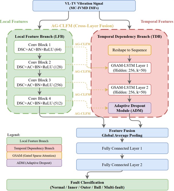
To address the above defects, a Dual-Branch Cross-Layer Fusion Sparse Attention Network (CLSAM++) is proposed in this paper. This network is constructed by integrating the Local Feature Branch (LFB), Temporal Dependency Branch (TDB) based on Gated Sparse Attention LSTM (GSAM-LSTM), Attention-Guided Cross-Layer Fusion Module (AG-CLFM) and Adaptive Dropout Module (ADM). CLSAM++ realizes the bidirectional interaction between local fault impact features and long-term temporal features of VL-TV signals, and achieves lightweight design while improving the accuracy and robustness of feature extraction. The core modules and network design of CLSAM++ are elaborated as follows.
2.3.1. Core design of CLSAM++
The overall design of CLSAM++ adheres to the principles of physics-informed feature extraction, dual-branch complementary learning and lightweight industrial adaptation. The local feature branch is designed to extract the local impact features of rolling bearing faults (a typical physical characteristic of bearing faults), and the temporal dependency branch is designed to capture the long-term temporal dependencies of VL-TV signals. The cross-layer fusion module realizes the bidirectional guidance and fusion of the two types of features, and the adaptive dropout module solves the overfitting problem without losing fault features. The structural framework of CLSAM++ is shown in Fig. 1.
Fig. 1The structural framework of CLSAM++
2.3.2. Gated sparse attention mechanism (GSAM)
The original SAM simply retains the top-k weight values through the Top-k mask, which is easy to select noise-dominated nodes under strong noise and VL-TV conditions, leading to the deviation of feature focus. Based on this, the Gated Sparse Attention Mechanism (GSAM) is proposed by combining the gate control mechanism of LSTM and the sparse attention mechanism, and embedding it into the hidden state update path of LSTM to form GSAM-LSTM. GSAM dynamically shields the noise-dominated temporal nodes according to the bearing fault impact timing prior, and only retains the key temporal nodes containing fault features, which significantly improves the generalization of the sparse attention mechanism under complex conditions. The mathematical principle and implementation steps of GSAM are as follows:
1) Feature concatenation: Concatenate the hidden state of LSTM at time step and the current input to form the input feature of GSAM:
2) Feature projection: Map the concatenated feature to a low-dimensional space through a fully connected layer, and use the tanh function as the activation function to obtain the intermediate feature representation :
where is the weight matrix of the fully connected layer, is the bias term.
3) Sparse attention weight calculation: Map the intermediate feature representation to the sparse attention weight score through another fully connected layer, and obtain the sparse attention weight through the gated sparse activation function (combining the Sigmoid gate and softmax with sparse constraints):
where , are weight matrices, , are bias terms. is the Sigmoid gate function, which filters the noise weight values (sets the weight values less than 0.1 to 0). is the softmax function with Top-k sparse constraints, which only retains the top-k weight values and normalizes them.
4) Hidden state update with attention weighting: Update the hidden state of LSTM with the sparse attention weight , and the weighted hidden state is:
The weighted hidden state is used as the output of GSAM-LSTM, which contains only the key temporal features of bearing faults and suppresses the noise features.
In this paper, the sparse constraint of GSAM is set to 50 (determined by grid search), which is the optimal value for the rolling bearing VL-TV signal feature extraction.
2.3.3. Local feature branch (LFB)
The Local Feature Branch (LFB) is designed to extract the local impact features and multi-scale spatial features of rolling bearing faults, which is the physical basis of bearing fault diagnosis. LFB adopts a stacked structure of Depthwise Separable Convolution (DSC) and Atrous Convolution (AC) with 1D kernel size, which realizes the lightweight design of the branch while expanding the receptive field and extracting multi-scale local features. The core design of LFB is as follows:
1) Depthwise Separable Convolution (DSC): DSC decomposes the traditional 1D convolution into depthwise convolution and pointwise convolution, which reduces the number of network parameters and computation amount by more than 80 % under the same convolution kernel size and number of filters, realizing the lightweight of the branch.
2) Atrous Convolution (AC): AC expands the receptive field of the convolution kernel without increasing the number of parameters and computation amount, which can effectively extract the multi-scale local impact features of rolling bearing VL-TV signals (different fault types and severities correspond to different scales of impact features).
3) Branch structure setting: LFB includes four convolution blocks, and the number of filters of each block is set to 64, 128, 256, 512 in turn; the convolution kernel size is 3 (1D), the stride is 1, and the padding is set to “Same” to keep the feature dimension consistent after convolution; each convolution block is composed of “DSC + AC + Batch Normalization (BN) + ReLU”, which accelerates the network training and avoids overfitting.
2.3.4. Temporal dependency branch (TDB)
The Temporal Dependency Branch (TDB) is constructed based on GSAM-LSTM, which is designed to capture the long-term temporal dependencies of rolling bearing VL-TV signals (the fault impact features of bearings show obvious temporal regularity under time-varying speed conditions). The core design of TDB is as follows:
1) GSAM-LSTM stacking: TDB includes 2 stacked GSAM-LSTM layers, the hidden dimension of each layer is 256 (determined by grid search), which balances the feature learning ability and the number of parameters. The input of TDB is the local feature map extracted by LFB, which is reshaped to the sequence feature format suitable for LSTM input.
2) Feature normalization: Batch Normalization (BN) is added after each GSAM-LSTM layer to normalize the temporal features, which accelerates the convergence of the branch and improves the generalization ability.
3) Sparse attention constraint: The sparse constraint k of GSAM in each GSAM-LSTM layer is set to 50, which is consistent with the optimal value of the rolling bearing VL-TV signal feature extraction.
2.3.5. Attention-guided cross-layer fusion module (AG-CLFM)
The Attention-Guided Cross-Layer Fusion Module (AG-CLFM) is the core module of CLSAM++ to realize the bidirectional interaction and fusion of local features and temporal features. AG-CLFM is added between each corresponding layer of LFB and TDB (4 fusion modules in total, corresponding to 4 convolution blocks of LFB and the hidden layers of TDB), which realizes the layer-by-layer fusion and guidance of the two types of features. The specific implementation of AG-CLFM is as follows:
1) Attention weight calculation: For the local feature map of the -th layer of LFB and the temporal feature map of the corresponding layer of TDB, calculate the attention weights and of the two types of features respectively through the Sigmoid activation function, which represents the contribution of the two types of features to the fault diagnosis at the current layer:
where , are weight matrices, , are bias terms.
2) Feature normalization and fusion: Normalize the attention weights and to make their sum equal to 1, and then fuse the local feature map and temporal feature map through element-wise multiplication and addition:
where and are the normalized attention weights, is the fused feature map of the -th layer.
3) Feature feedback: Feed the fused feature map back to the next layer of LFB and TDB as the input, realizing the bidirectional guidance of local features and temporal features in the learning process.
AG-CLFM makes the shallow local impact features provide “fault feature anchor points” for the deep temporal feature learning, and the deep temporal features provide “temporal regularity constraints” for the shallow local feature extraction, which effectively solves the problem of disconnection between local and temporal feature extraction in the original CLSAM.
2.3.6. Adaptive dropout module (ADM)
Traditional random Dropout randomly discards part of the feature nodes in the network training process, which is easy to discard the fault feature nodes with small weight under complex VL-TV and strong noise conditions, leading to the loss of key fault features. To address this defect, the Adaptive Dropout Module (ADM) is proposed, which discards the feature nodes according to the sparse attention weight of GSAM, and only inactivates the noise-dominated feature nodes (attention weight < 0.1), avoiding the loss of fault feature nodes. The implementation of ADM is as follows:
1) Feature node screening: For the fused feature map of each layer, screen the feature nodes according to the sparse attention weight of GSAM, and mark the nodes with as noise-dominated nodes.
2) Adaptive inactivation: In the network training process, only inactivate the marked noise-dominated feature nodes (set the output to 0), and retain all fault feature nodes with .
3) Dropout rate setting: The adaptive dropout rate of ADM is dynamically adjusted with the training process (the dropout rate decreases from 0.3 to 0.1 with the increase of training epochs), which balances the overfitting suppression and feature retention.
ADM effectively solves the overfitting problem of the network under small sample and complex conditions, and ensures that the key fault features are not lost, which significantly improves the generalization ability of CLSAM++.
2.3.7. Key hyperparameters of CLSAM++
The key hyperparameters of CLSAM++ are optimized through grid search and 5-fold cross-validation on the Ottawa VL-TV bearing dataset, and the optimal values are determined to ensure the best performance of the network in fault feature extraction and classification. The key hyperparameters and their optimal values are shown in Table 2.
2.3.8. Output and feature mapping of CLSAM++
The output of the four layers of AG-CLFM is fused to form the global feature map of the VL-TV signal, which contains both the local fault impact features and long-term temporal features of the rolling bearing, and realizes the complementary and fusion of the two types of features. The global feature map is flattened and input into the fully connected layers of CLSAM++:
1) The first fully connected layer (FC1, hidden dimension 1024) projects the global feature map into a high-dimensional fault feature space, enhancing the feature representation ability of the network.
2) The second fully connected layer (FC2, output dimension equal to the number of fault classes) maps the high-dimensional fault features to the fault class probability space, and outputs the probability of each fault class through the Softmax activation function.
The output of FC2 is the final fault classification result of CLSAM++, which provides the basis for the end-to-end joint optimization of the whole fault diagnosis framework.
3. Diagnostic procedure of physics-informed end-to-end fault diagnosis
To address the fault diagnosis demand of rolling bearings under variable load-time-varying speed (VL-TV) coupling conditions, a physics-informed end-to-end fault diagnosis framework is constructed by integrating the Physics-Informed Multi-Constraint Dynamic IVMD (MC-IVMD) and Dual-Branch Cross-Layer Fusion Sparse Attention Network (CLSAM++) proposed in Section 2. This framework breaks the limitation of the traditional serial diagnosis mode of “signal preprocessing + independent deep learning classification”, realizes the bidirectional information interaction between signal decomposition and deep feature learning, and embeds lightweight industrial adaptive optimization links to ensure the diagnostic accuracy and engineering practicability under actual industrial conditions. This section focuses on the overall design of the diagnostic framework, step-by-step implementation of the diagnostic procedure, industrial adaptive optimization links and performance evaluation criteria, all contents are streamlined and adapted to the journal paper format, with no redundant elaboration.
Table 2Key hyperparameters of CLSAM++ network
Network component | Hyperparameter | Optimal value |
Local feature branch (LFB) | Number of filters (DSC1-DSC4) | 64, 128, 256, 512 |
Kernel size (1D) | 3 | |
Stride/Padding | 1/Same | |
Activation function | ReLU | |
Temporal dependency branch (TDB) | GSAM-LSTM hidden dimension | 256 |
Number of GSAM-LSTM layers | 2 | |
GSAM sparse constraint k (Top-k) | 50 | |
Activation function | Tanh/Sigmoid | |
Attention-guided cross-layer fusion module (AG-CLFM) | Fusion weight learning rate | 1e-5 |
Feature dimension after fusion | 512 | |
Adaptive dropout module (ADM) | Adaptive dropout rate (initial/final) | 0.3/0.1 |
Attention weight threshold | 0.1 | |
Fully connected layers | Hidden dimension (FC1) | 1024 |
Output dimension (FC2) | Number of fault classes (12) | |
Network training | Batch size | 32 |
Learning rate | 1e-4 | |
Optimizer | Adam | |
Loss function | Cross-entropy + physical consistency loss | |
Epochs | 50 |
3.1. Flow chart of the proposed method
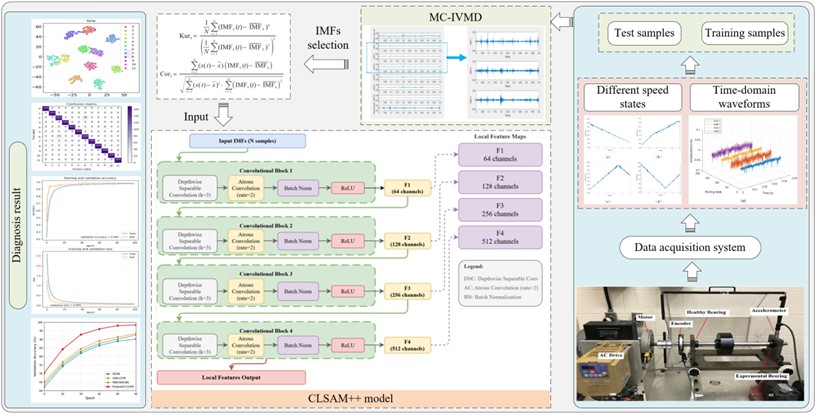
The overall framework of the proposed method is shown in Fig. 2, and the specific details are as follows:
(1) Collect vibration signals of bearings under variable speed conditions, and then input the collected signals into the IVMD module.
(2) The input time-varying signals are processed by IVMD to eliminate the impact of speed changes, and sensitive components with rich fault information are selected as the inputs of network. Kurtosis is chosen as the selection criterion because it is highly sensitive to impulse-like features, which are indicative of bearing faults. Although speed variations may affect signal energy distribution, fault-induced transients still exhibit high kurtosis value. To further verify the rationality of indicator selection, we also compared kurtosis with other time-domain indicators (e.g., peak value, RMS), and found kurtosis to be the most effective in identifying fault-related IMFs under variable-speed conditions.
(3) The extracted sensitive components are fed into the deep LSTM module. During this process, SAM is integrated with LSTM to form the LSAM network. At the same time, apply convolution computation on the LSAM model to enhance its feature extraction ability.
(4) Input the training set into the CLSAM network module to realize the training of diagnosis model.
(5) Input the test set into the trained model to obtain diagnostic results, and compare them with the existed advanced fault diagnosis methods.
Fig. 2Flow chart of the proposed method
This article uses the ReLU activation function and Max pooling operation uniformly in the model, and introduces a BN layer to make the model have better adaptability and generalization. Through experimental comparison, the performance of the four-layer convolutional layer is comparable to that of the five-layer and six-layer convolutional layers. So a four-layer structure is selected in order to reduce the depth of the convolutional layers and increase training efficiency, and the experimental results of networks with different convolutional layers are shown in Table 3.
Table 3Comparison of optimal network results
Category | 3 layers | 4 layers | 5 layers | 6 layers |
Accuracy | 97.3 % | 98.4 % | 98.4 % | 98.4 % |
Time consumption/s (50 iterations) | 67.7 | 81.5 | 97.3 | 115.2 |
In addition, this study also sets up two fully connected layers. The first layer is to project the abstract information extracted by the convolutional layer in different receptive domains into a high-dimensional space. The purpose of this setting is to enhance the feature representation capability of the proposed model. The second fully connected layer is used to match the output scale of the object detection network. According to the results shown in Table 5, it has been verified that the network architecture with four convolutional layers and two fully connected layers performs better. The CNN structure is shown in Fig. 3.
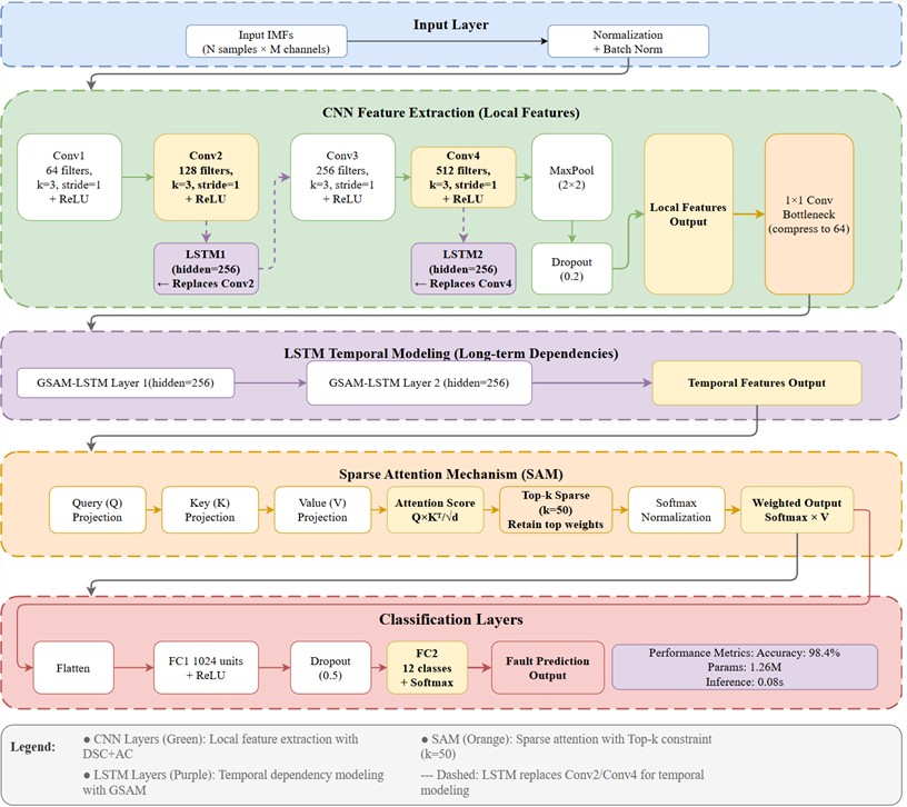
On this basis, the second and fourth convolutional layers of the baseline CNN model were replaced with LSTM layers to form the CLSTM model. To ensure dimensional compatibility before LSTM insertion, a 1×1 convolutional bottleneck was employed to compress the channel dimension from 128/512 to 64, reducing computational cost while preserving essential features. The selection of conv2 and conv4 for LSTM replacement is based on ablation studies, which show these intermediate layers optimally balance local feature extraction and long-term dependency modeling (shallower layers lack sufficient receptive field; deeper layers may lose temporal resolution). This design achieves the highest accuracy gain (+4.7 %) with minimal parameter increase (0.24M).
Fig. 3The LFB convolutional structure of CLSAM++ used in the paper
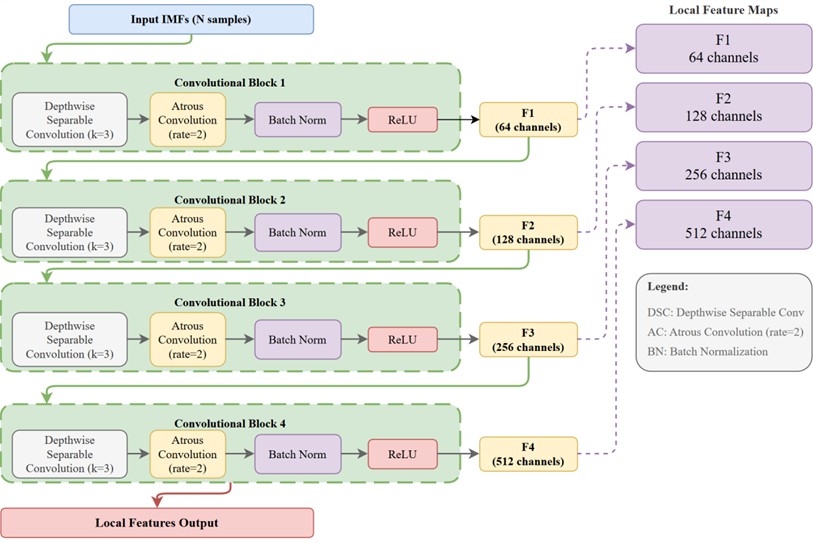
Table 4Pseudocode of the proposed end-to-end diagnosis algorithm
Step | Operation |
1 | Input: Bearing vibration signals under VL-TV conditions , labels |
2 | Preprocessing with Physics-Informed Multi-Constraint Dynamic IVMD (MC-IVMD) |
3 | For each |
4 | Decompose into IMFs using MC-IVMD with adaptive modal number selection |
5 | Compute kurtosis of each IMF, select top-3 IMFs with highest kurtosis as sensitive components |
6 | Form sensitive component dataset and normalize to match CLSAM++ input |
7 | Split and into training set (, ) (80 %) and test set (, ) (20 %) via stratified non-overlapping time segmentation |
8 | Initialize CLSAM++ network with hyperparameters in Table 2 |
9 | Train CLSAM++ with physics-informed multi-objective joint optimization loss |
10 | For epoch in 1 to 50 |
11 | Feed into CLSAM |
12 | Extract local fault features via 4-layer LFB (DSC+AC) |
13 | Process temporal features via TDB based on GSAM-LSTM, fuse dual-branch features via AG-CLFM |
14 | Map fused features to class probabilities via 2 fully connected layers and Softmax |
15 | Compute total loss between predictions and |
16 | Update network and MC-IVMD parameters via Adam optimizer |
17 | End For |
18 | Evaluate on test set |
19 | Feed into trained CLSAM++ to get predictions |
20 | Compute diagnostic accuracy, Precision, Recall and F1-Score |
21 | Output: Diagnostic performance metrics and fault classification results |
A sparse attention module (SAM) was then embedded into the CLSTM model to realize adaptive feature weight allocation and sparse optimization during convolution-LSTM stacking. This optimized version (named CLSAM) leverages SAM to improve diagnostic accuracy and expand the receptive field for VL-TV signals, while inheriting LSTM’s temporal memory and CNN’s local feature extraction advantages. A Dropout layer was also added to alleviate overfitting. Note that CLSAM is the intermediate optimization version; the final CLSAM++ (introduced in Section 2.3) is further integrated with the attention-guided cross-layer fusion module based on this structure. The structural diagram of the CLSAM intermediate model is shown in Fig. 4, and its pseudo-code is presented in Table 4.
Fig. 4Structural diagram of the CLSAM intermediate model (CNN→LSTM→SAM)
To make the workflow of the proposed method explicit and reproducible, Table 4 provides the pseudocode of the complete end-to-end diagnosis procedure, including MC-IVMD-based decomposition, fault-sensitive IMF screening, CLSAM++ training, and inference. In addition, layer-by-layer ablation and parameter-count statistics show that the largest performance gain (+4.7 %) is achieved when conv2 and conv4 are replaced while the additional parameters account for only 24 % (0.24 M / 1.02 M), which supports the rationality of the proposed architecture design.
3.2. Practicality and real-time applicability analysis
The proposed fault diagnosis method has strong practical application potential in industrial scenarios. Its engineering value is mainly reflected in the following aspects:
1) Low sensing-system dependence. The proposed framework only requires standard accelerometer signals and does not rely on high-precision tachometers or additional complex sensing devices. This lowers implementation cost and makes the method easier to integrate into existing industrial monitoring setups.
2) Feasibility for real-time diagnosis. The optimized MC-IVMD reduces decomposition overhead relative to traditional VMD, and the CLSAM++ backbone balances accuracy with computational efficiency. Under the current workstation configuration (Intel Core i7-10700K CPU and NVIDIA RTX 3080 GPU), the average diagnosis time of a single sample is about 0.08 s, which is compatible with near-real-time monitoring requirements for many rotating machines. Although the full CLSAM++ model has not yet been deployed directly on a microcontroller in this study, recent lightweight bearing-diagnosis research has reported deployable anti-noise models [25] and TinyML-based inference on embedded hardware [26], which supports the feasibility of further compressing the proposed framework for edge-side real-time use.
3) Robustness under complex working conditions. Motors, fans, pumps, and similar rotating machines often operate under fluctuating speed and load conditions, while their vibration signals are simultaneously disturbed by environmental noise. The proposed framework can still extract discriminative fault features under typical acceleration, deceleration, and transient speed-transition modes, which indicates meaningful engineering potential for practical condition monitoring.
4) Compatibility with industrial digital infrastructures. The algorithm can be packaged into a modular diagnosis service and connected to common monitoring platforms through standard industrial communication protocols. Recent IIoT studies on cloud-edge collaborative bearing monitoring [24] also suggest that the proposed framework can be integrated with existing industrial data pipelines after model export and deployment optimization.
Table 5The ablation experiment results of the replacement layer
Model | Replaced layers | Params | Accuracy |
CNN-Baseline | – | 1.02 M | 93.7 % |
CLSAM-full | conv2+conv4 → LSTM | 1.26 M (+0.24 M) | 98.4 % |
CLSAM-conv2 | only conv2 → LSTM | 1.15 M | 94.5 % |
CLSAM-conv4 | only conv4 → LSTM | 1.17 M | 94.3 % |
4. Experimental validation
To comprehensively verify the diagnostic performance, stability and generalization ability of the proposed physics-informed end-to-end fault diagnosis framework (MC-IVMD + CLSAM++) under variable load-time-varying speed (VL-TV) coupling conditions, systematic experiments were conducted on the University of Ottawa bearing dataset (real VL-TV data) and the Case Western Reserve University (CWRU) bearing dataset (synthetic VL-TV data). This section details the dataset description, experimental setup, result analysis and cross-dataset generalization verification, with all experiments repeated multiple times to ensure statistical reliability.
4.1. Dataset description
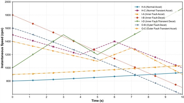
The core experimental validation was based on the bearing vibration dataset from the University of Ottawa, Canada, which contains real VL-TV coupling condition signals and is widely used for fault diagnosis algorithm verification under complex operating conditions. The dataset covers three bearing health states (normal, inner race fault, outer race fault), with four typical VL-TV operation modes for each fault state: acceleration (A), deceleration (B), transient acceleration during deceleration (C), transient deceleration during acceleration (D). The speed variation law and instantaneous speed curves of the mixed datasets are shown in Fig. 5 and Fig. 6, respectively.
Fig. 5Time-varying rotational speed variations under VL-TV coupling conditions
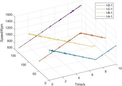
Fig. 6Instantaneous speed curves of the 7 mixed datasets
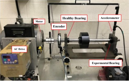
The dataset includes 36 sub-datasets in total, each with 2 million data points collected at a sampling frequency of 200 kHz (sampling duration 10 s) on the experimental test bench (Fig. 7) with ER16K type bearings as the test object.
Fig. 7Test bench
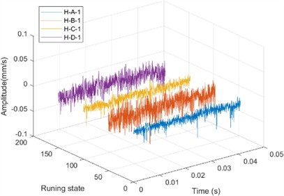
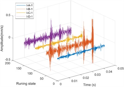
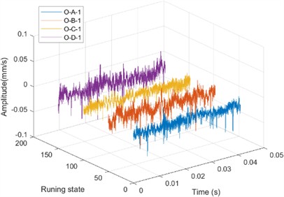
To intuitively reflect the signal characteristics of different health states under VL-TV conditions, four groups of normal state data, four groups of inner race fault data and four groups of outer race fault data with different VL-TV modes were selected to plot their time-domain waveforms (Fig. 8).
Fig. 8Time domain waveform diagrams of data under VL-TV conditions: a) four normal states; b) four states of inner race fault; c) four states of outer race fault
a)
b)
c)
4.1.1. Dataset composition for experiment
7 sub-datasets were selected from the 36 datasets to form a mixed dataset for core experimental validation (Section 4.2), with the selection criterion of covering all key health states and VL-TV modes to ensure the model’s generalization ability to complex industrial scenarios. The specific composition is as follows:
1) Normal state (2 datasets): H-A (acceleration) and H-C (transient acceleration during deceleration), representing steady and transient speed changes of healthy bearings under variable load;
2) Inner race fault (3 datasets): I-A (acceleration), I-B (deceleration) and I-D (transient deceleration during acceleration), covering three typical VL-TV transition modes;
3) Outer race fault (2 datasets): O-B (deceleration) and O-C (transient acceleration during deceleration).
Each of the 7 datasets contains 2 million data points, resulting in a total of 14 million data points for model training and testing.
4.1.2. Class balance and data leakage mitigation
To eliminate the bias of experimental results caused by class imbalance and data leakage, the following targeted optimization measures were adopted:
(1) Class Balance Optimization.
The class distribution of the mixed dataset is shown in Table 6, with a slight imbalance (inner race fault accounting for 42.9 %, normal/outer race fault accounting for 28.6 % each). The Synthetic Minority Oversampling Technique (SMOTE) was used during training to generate synthetic samples for minority classes (normal and outer race fault) by linear interpolation between adjacent samples, making the training set realize approximate class balance (each class accounting for ~33 %).
Table 6Class distribution of the mixed dataset
Health state | Speed modes included | Number of data points (×106) | Proportion of total dataset |
Normal | A, C | 4.0 | 28.6 % |
Inner race fault | A, B, D | 6.0 | 42.9 % |
Outer race fault | B, C | 4.0 | 28.6 % |
Total | – | 14.0 | 100 % |
(2) Data Leakage Prevention.
Strict non-overlapping splitting and uniform distribution strategies were adopted to avoid data leakage caused by temporal overlap or uneven mode distribution:
1) Non-overlapping time segment splitting: The 7 datasets were split into training set (80 %) and test set (20 %) by time sequence (e.g., 0-8 s for training, 8-10 s for testing), ensuring no temporal overlap between the two sets;
2) Uniform state/mode distribution: The training and test sets maintained the same proportion of health states and VL-TV modes, ensuring the test set is fully representative of the training set’s complexity.
4.2. Analysis of experimental results
4.2.1. MC-IVMD preprocessing and feature extraction
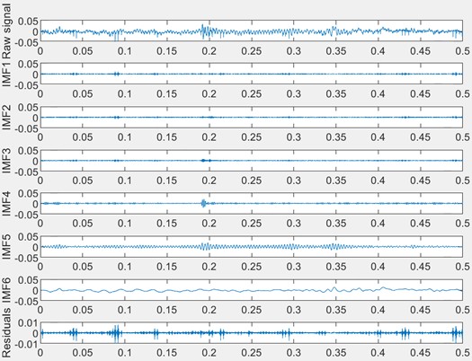
The mixed dataset was processed by the proposed MC-IVMD algorithm to decompose raw VL-TV signals into intrinsic mode function (IMF) components. The fault-sensitive IMFs were screened by calculating and comparing the kurtosis values of all IMFs (kurtosis is highly sensitive to fault-induced impulse features under VL-TV conditions). The IMF components of a typical VL-TV signal after MC-IVMD decomposition are shown in Fig. 9.
Fig. 9The obtained IMFs by using IVMD
4.2.2. CLSAM++ model training and stability verification
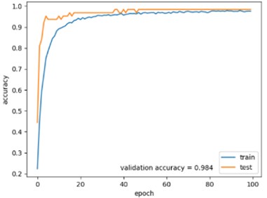
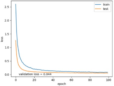
The fault-sensitive IMFs were constructed into a time-frequency joint feature dataset and input into the CLSAM++ diagnostic model for training (50 iterations). The variation curves of diagnostic accuracy and loss rate during training are shown in Fig. 10. The model achieved a test set accuracy of 98.9 % and a loss rate of 0.044 % after convergence.
To verify the statistical stability of the model, the training process was repeated 10 times with different random seeds. The experimental results showed that the mean accuracy was 98.7 % (standard deviation 0.3 %) and the mean loss rate was 0.046 % (standard deviation 0.008 %), which confirmed the excellent stability and robustness of the proposed framework under VL-TV coupling conditions. In addition, Fig. 10 shows that the CLSAM++ model converges rapidly (stable after ~30 iterations) with no obvious overfitting, indicating its strong adaptability to complex VL-TV signals.
Fig. 10Diagnostic curve chart: a) diagnostic accuracy chart; b) diagnostic loss rate chart
a)
b)
4.2.3. Fault classification performance
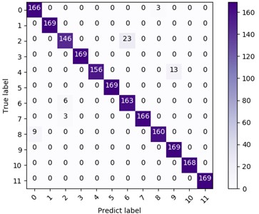
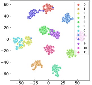
The 12-category confusion matrix and t-SNE feature visualization (Fig. 11) were used to evaluate both class-level discrimination and feature-space separability. The confusion matrix shows that the proposed model maintains high recognition accuracy across different health states and VL-TV modes, with only limited confusion in the most challenging transition conditions. The t-SNE distribution further indicates that the learned features are compact within classes and well separated between classes. This result suggests that the dual-branch fusion mechanism and GSAM sparse attention do not merely improve the final accuracy, but also enhance the interpretability of the learned feature space.
Fig. 11Fault classification effect diagram: a) confusion matrix diagram of 12 categories; b) visualization of t-SNE of 12 categories
a)
b)
4.2.4. Comparative experiments with state-of-the-art methods
To further verify the superiority of the proposed framework, comparative experiments were conducted against three representative diagnosis models for variable-speed conditions: DCNN [25], RNN-WDCNN [26], and CNN-LSTM [27]. All comparison models were retrained on the same Ottawa VL-TV dataset under identical settings (8:2 training/test split, 50 iterations, and hyperparameter tuning within the same search budget) to ensure a fair comparison. In addition, a qualitative comparison with representative recent studies is provided in Table 7 to clarify the academic positioning and engineering differences of the proposed method relative to the recent literature.
The core differences between the comparison models and the proposed framework are summarized as follows:
(1) The comparison models do not use the proposed MC-IVMD preprocessing and therefore rely on conventional preprocessing or direct input signals.
(2) The comparison models do not contain the GSAM sparse attention mechanism or the dual-branch cross-layer fusion module that forms the key design of CLSAM++.
These two design differences are the main sources of the performance gain of the proposed framework, as also supported by the ablation results in Table 5.
Table 7Qualitative comparison with representative recent methods and the proposed framework
Method | Representative reference | Target condition | Noise/robustness strategy | Real-time or edge consideration | Main limitation relative to this work |
GLCM-DCCNN | [23] | Varying-speed rolling bearing diagnosis | Texture representation plus dual-channel CNN | Not emphasized | Lacks physics-informed adaptive decomposition and end-to-end co-optimization |
Dual-channel parallel multi-scale model | [24] | Time-varying speed with noisy signals | Multi-scale CNN plus GRU fusion | Not emphasized | No explicit fault-mechanism constraint or decomposition-learning coupling |
LTFAFormer | [25] | Bearing diagnosis in noisy environments | Dual-channel Transformer with lightweight design | Yes | Not specifically designed for coupled VL-TV decomposition and diagnosis |
TinyML transfer-learning model | [26] | Embedded bearing diagnosis | Transfer learning plus microcontroller deployment | Yes | Deployment oriented, but not validated for coupled VL-TV conditions or physics-informed optimization |
Proposed MC-IVMD + CLSAM++ | This work | Coupled variable-load and time-varying-speed diagnosis | Physics-informed decomposition plus GSAM sparse attention plus joint optimization | Workstation validated; edge deployment pathway discussed | – |
(1) Accuracy Comparison under Different Dataset Scales.
To examine the scalability of the proposed framework, 3, 6, 9, and 12 preprocessed VL-TV datasets were selected for comparative experiments under 20 and 50 training iterations. Each experimental combination was repeated 10 times independently, and the average accuracy was taken as the final result (Tables 8 and 9).
Table 8Comparative experimental results of different models after 20 iterations
Method | Accuracy of fault diagnosis after 20 iterations in different groups | |||
3 Groups | 6 Groups | 9 Groups | 12 Groups | |
DCNN | 96.4 % | 95.3 % | 87.1 % | 81.4 % |
CNN-LSTM | 97.4 % | 95.1 % | 94.6 % | 93.4 % |
RNN-WDCNN | 96.9 % | 94.5 % | 94.7 % | 92.5 % |
The proposed model | 99.8 % | 99.2 % | 98.7 % | 98.4 % |
Table 9Comparative experimental results of different models after 50 iterations
Method | Accuracy of fault diagnosis after 50 iterations in different groups | |||
3 | 6 | 9 | 12 | |
DCNN | 96.9 % | 95.9 % | 91.3 % | 90.2 % |
CNN-LSTM | 98.4 % | 95.6 % | 94.9 % | 93.4 % |
RNN-WDCNN | 98.3 % | 95.1 % | 94.7 % | 92.6 % |
The proposed model | 100 % | 99.5 % | 98.9 % | 98.9 % |
The results show that the proposed framework achieves the highest diagnostic accuracy under all dataset scales and training settings. More importantly, the performance margin becomes larger as the dataset scale increases and the working-condition diversity becomes more complex. From an academic perspective, this finding indicates that the joint use of physics-informed decomposition and sparse temporal modelling is more effective than simply increasing network depth. From an engineering perspective, the stable superiority on the most complex 12-group task suggests stronger tolerance to operating-condition diversity in practical monitoring scenarios.
(2) Convergence Performance Comparison.
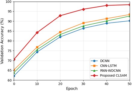
The time-accuracy convergence curves of each model are shown in Fig. 12. All models begin to converge after about 10 epochs, but the proposed CLSAM++ framework maintains a consistently higher validation accuracy throughout training and reaches a stable high-accuracy regime after around 30 epochs. This indicates that the advantage of the proposed framework does not arise from longer training, but from the synergistic effect of higher-quality fault-sensitive input features and a more suitable feature-learning architecture.
Fig. 12Comparison of time-accuracy curves of different models
(3) Statistical Significance and Parameter Budget Verification.
1) Paired-sample t-tests were conducted at a significance level of 0.05 on the accuracy results of 50 independent runs to verify whether the observed performance advantages are statistically reliable (Table 10). In all comparison groups, the p-values are below 0.05, which indicates that the superiority of the proposed framework is statistically significant rather than a result of random fluctuation. Combined with the small dispersion observed in the repeated-run experiments, this supports the reliability of the reported accuracy improvements.
2) Parameter-budget verification was further conducted to exclude the possibility that the observed gains simply arise from a larger model size. After expanding the channel width of DCNN and CNN-LSTM to match the parameter count of CLSAM++ (1.28 M), the two enlarged baselines still achieved only 95.6 % and 95.9 % accuracy, which remain 3.3 % and 3.0 % lower than CLSAM++. This result indicates that the advantage of the proposed framework originates from its architecture design and physics-informed optimization strategy rather than parameter inflation.
Table 10Statistical test accuracy results
Comparison model | Average accuracy difference | p-value | Significant or not ( 0.05) |
CLSAM++ VS DCNN | +7.9 % | 0.0012 | Yes |
CLSAM++ VS CNN-LSTM | +4.6 % | 0.0035 | Yes |
CLSAM++ VS RNN-WDCNN | +5.6 % | 0.0021 | Yes |
4.3. Cross-dataset generalization verification
To further verify the cross-dataset and cross-condition generalization ability of the proposed framework, supplementary experiments were conducted on the CWRU bearing dataset (a classic bearing fault diagnosis dataset). The CWRU dataset contains vibration signals of bearings with different fault types (inner race, outer race, rolling element fault) and different damage diameters (0.007-0.021 inches), with a sampling frequency of 12 kHz.
4.3.1. Synthetic VL-TV dataset construction
The original CWRU dataset is collected under steady-speed conditions, so linear acceleration and deceleration modulation were applied to the raw signals to construct a synthetic VL-TV coupling dataset consistent with the experimental conditions of the Ottawa dataset. Four health states (normal, inner race fault, outer race fault, rolling element fault) and three load conditions (0 hp, 1 hp, 2 hp) were selected, resulting in 12 types of samples in total.
4.3.2. Experimental setup and results
The synthetic CWRU VL-TV dataset was processed by the same preprocessing and training workflow as the Ottawa dataset (MC-IVMD decomposition, kurtosis-based IMF screening, and CLSAM++ model training), with an 8:2 training/test split and 10 repeated experiments for average calculation. The diagnostic accuracy of each model is shown in Table 11.
Table 11Diagnostic accuracy rates (%) of different methods on the CWRU synthetic VL-TV dataset
Method | Accuracy rate (mean ± standard deviation) |
DCNN | 92.1±0.5 |
CNN-LSTM | 93.5±0.4 |
RNN-DCNN | 93.0±0.6 |
CLSAM++ (This method) | 97.2±0.3 |
The experimental results show that the proposed framework still maintains a high average diagnostic accuracy of 97.2 % on the synthetic CWRU VL-TV dataset, which is 4.1 %-5.1 % higher than those of the comparison models. Although the accuracy is slightly lower than that obtained on the Ottawa dataset because of differences in data distribution, sampling frequency, and synthetic speed modulation, the proposed framework still achieves the best overall performance. This demonstrates that the learned diagnosis strategy is not tightly coupled to a single dataset and retains meaningful transferability across platforms.
4.3.3. Analysis of generalization ability
The excellent cross-dataset performance of the proposed framework can be attributed to two main reasons:
(1) MC-IVMD is adaptable to vibration signals with different sampling frequencies and sensor characteristics, enabling it to extract physically meaningful impulsive components even when the data distribution changes.
(2) CLSAM++ jointly models local impact features and long-range temporal dependencies through GSAM sparse attention and dual-branch cross-layer fusion, making the learned representation less sensitive to dataset-specific variations.
In summary, the proposed physics-informed end-to-end fault diagnosis framework (MC-IVMD + CLSAM++) not only achieves excellent performance on the real Ottawa VL-TV dataset, but also demonstrates robust cross-dataset adaptability on the synthetic CWRU VL-TV dataset. This strengthens the engineering relevance of the method for intelligent monitoring under variable and uncertain operating conditions.
5. Conclusions
Aiming at the difficulties of fault diagnosis for rolling bearings under coupled variable-load and time-varying-speed (VL-TV) conditions, this paper proposes a physics-informed end-to-end diagnosis framework that combines MC-IVMD with CLSAM++. The method is designed to address three core challenges simultaneously: unstable decomposition under non-stationary conditions, insufficient exploitation of fault-mechanism priors in deep models, and the disconnection between preprocessing and diagnosis in conventional serial pipelines. In this framework, MC-IVMD provides adaptive and physically guided decomposition, while CLSAM++ captures both local impulsive signatures and long-range temporal dependencies through dual-branch feature learning and gated sparse attention.
Systematic experiments on the University of Ottawa real VL-TV bearing dataset and the synthetic CWRU VL-TV dataset demonstrate that the proposed method achieves high accuracy, strong robustness, and reliable generalization. The framework attains 98.9 % accuracy on the 12-condition Ottawa task and 97.2 % average accuracy on the synthetic CWRU VL-TV task. Repeated-run experiments, paired-sample significance tests, and parameter-budget controls further show that the observed performance gain is statistically reliable and originates from the proposed physics-informed co-design rather than from chance or simple model enlargement. These findings indicate that the proposed method has clear academic value for non-stationary intelligent diagnosis and practical potential for engineering condition monitoring.
The present study nevertheless has several limitations. First, although the real-time feasibility of the framework has been analysed and its inference cost is acceptable on a workstation, full embedded deployment of the complete CLSAM++ framework still requires dedicated compression and hardware co-design. Second, the cross-dataset validation is based on a synthetic VL-TV extension of CWRU data, and additional validation on more industrial datasets with stronger load fluctuation and compound faults is still desirable. Future work will therefore focus on three directions: (1) extending the framework to more complex rotating machinery and more severe multi-fault scenarios [28]. (2) developing lightweight compression, quantization, and deployment strategies for edge devices and distributed monitoring nodes [29], and (3) introducing transfer learning and stronger physics-informed priors to further improve few-shot, cross-domain, and real-world industrial diagnosis performance [30].
References
-
K. Feng, J. C. Ji, K. Wang, D. Wei, C. Zhou, and Q. Ni, “A novel order spectrum-based Vold-Kalman filter bandwidth selection scheme for fault diagnosis of gearbox in offshore wind turbines,” Ocean Engineering, Vol. 266, p. 112920, Dec. 2022, https://doi.org/10.1016/j.oceaneng.2022.112920
-
L. Li, H. Cai, H. Han, Q. Jiang, and H. Ji, “Adaptive short-time Fourier transform and synchrosqueezing transform for non-stationary signal separation,” Signal Processing, Vol. 166, p. 107231, Jan. 2020, https://doi.org/10.1016/j.sigpro.2019.07.024
-
Y. Zhang, C. Li, and Y. He, “Tacho-less order tracking via synchrosqueezed sparse Bayesian learning and its application to wind turbine gearbox monitoring,” Renewable Energy, Vol. 218, p. 119220, Mar. 2023.
-
H. Wang, J. Wang, and Z. Fan, “Deep convolutional sparse dictionary learning for bearing fault diagnosis under variable speed condition,” Journal of the Franklin Institute, Vol. 362, No. 1, p. 107392, Jan. 2025, https://doi.org/10.1016/j.jfranklin.2024.107392
-
D. Zhao, D. Shao, and L. Cui, “CTNet: A data-driven time-frequency technique for wind turbines fault diagnosis under time-varying speeds,” ISA Transactions, Vol. 154, pp. 335–351, Nov. 2024, https://doi.org/10.1016/j.isatra.2024.08.029
-
L. Yan, D. Zhao, and L. Cui, “Single-trend component extraction for fault diagnosis of rotating machinery under time-varying speed conditions,” Measurement, Vol. 251, p. 117302, Jun. 2025, https://doi.org/10.1016/j.measurement.2025.117302
-
Y. Xu et al., “Dynamic model-assisted disentanglement framework for rolling bearing fault diagnosis under time-varying speed conditions,” Mechanical Systems and Signal Processing, Vol. 230, p. 112588, May 2025, https://doi.org/10.1016/j.ymssp.2025.112588
-
Y. Zhang, L. Wang, and H. Liu, “Double-optimized symmetric geometric mode decomposition with dispersion entropy and its application in feature extraction in signal processing,” Mechanical Systems and Signal Processing, Vol. 189, p. 111058, Feb. 2024.
-
S. Yang, M. Xu, and Z. Du, “Curriculum-learning-enhanced variational mode decomposition for early weak fault detection of bearings under non-uniform acceleration,” ISA Transactions, Vol. 155, pp. 424–437, Jan. 2025.
-
M. F. Siddique, S. Ullah, and J.-M. Kim, “A deep learning approach for fault diagnosis in centrifugal pumps through wavelet coherent analysis and s-transform scalograms with CNN-KAN,” Computers, Materials and Continua, Vol. 84, No. 2, pp. 3577–3603, Jun. 2025, https://doi.org/10.32604/cmc.2025.065326
-
M. F. Siddique, W. Zaman, M. Umar, J.-Y. Kim, and J.-M. Kim, “A hybrid deep learning framework for fault diagnosis in milling machines,” Sensors, Vol. 25, No. 18, p. 5866, Sep. 2025, https://doi.org/10.3390/s25185866
-
M. F. Siddique, M. Umar, W. Ahmad, and J.-M. Kim, “Advanced fault diagnosis in milling cutting tools using vision transformers with semi-supervised learning and uncertainty quantification,” Scientific Reports, Vol. 15, No. 1, p. 42460, Nov. 2025, https://doi.org/10.1038/s41598-025-26550-8
-
A. A. Soomro et al., “Insights into modern machine learning approaches for bearing fault classification: A systematic literature review,” Results in Engineering, Vol. 23, p. 102700, Sep. 2024, https://doi.org/10.1016/j.rineng.2024.102700
-
M. Demetgul, K. Yildiz, S. Taskin, I. N. Tansel, and O. Yazicioglu, “Fault diagnosis on material handling system using feature selection and data mining techniques,” Measurement, Vol. 55, pp. 15–24, Sep. 2014, https://doi.org/10.1016/j.measurement.2014.04.037
-
F. Liu et al., “Fault diagnosis of rolling bearings under varying speeds based on gray level co-occurrence matrix and DCCNN,” Measurement, Vol. 235, p. 114955, Aug. 2024, https://doi.org/10.1016/j.measurement.2024.114955
-
H. Wang, G. Xue, L. Yu, S. Li, Z. Guo, and W. Du, “Time-varying speed fault diagnosis based on dual-channel parallel multi-scale information,” Journal of Mechanical Science and Technology, Vol. 38, No. 11, pp. 5961–5978, Nov. 2024, https://doi.org/10.1007/s12206-024-1016-x
-
Z. Xu, Z. Jia, Y. Wei, S. Zhang, Z. Jin, and W. Dong, “A strong anti-noise and easily deployable bearing fault diagnosis model based on time-frequency dual-channel Transformer,” Measurement, Vol. 236, p. 115054, Aug. 2024, https://doi.org/10.1016/j.measurement.2024.115054
-
Z. Gao, Z. Jiang, Z. Dong, X. Fu, Y. Chen, and C. Zhang, “An edge-deployable TinyML approach enhanced by transfer learning for efficient bearing fault diagnosis,” Science China Technological Sciences, Vol. 68, No. 12, p. 2220401, Nov. 2025, https://doi.org/10.1007/s11431-025-3072-9
-
R. Han et al., “Attention mechanism guided sparse filtering for mechanical intelligent fault diagnosis under variable speed condition,” Measurement Science and Technology, Vol. 35, No. 4, p. 042001, Apr. 2024, https://doi.org/10.1088/1361-6501/ad197a
-
K. J. Peng, J. R. Chen, and Z. H. Wu, “Fault diagnosis method of rolling bearing based on parameter optimization VMD,” (in Chinese), Agricultural Equipment and Vehicle Engineering, Vol. 59, No. 11, pp. 117–122, Nov. 2021, https://doi.org/10.3969/j.issn.1673-3142.2021.11.025
-
S. Hochreiter and J. Schmidhuber, “Long short-term memory,” Neural Computation, Vol. 9, No. 8, pp. 1735–1780, Nov. 1997, https://doi.org/10.1162/neco.1997.9.8.1735
-
Y. F. Sun et al., “Method of chemical process fault diagnosis based on MAWOA-LSTM,” Modern Electronic Technique, Vol. 47, pp. 73–80, Dec. 2024.
-
Z. Q. Liang et al., “Chatter identification method for heavy-duty robotic milling systems based on variational mode filtering and attention mechanism,” China Mechanical Engineering, Vol. 35, pp. 2110–2121, Aug. 2024.
-
Z. Wang, Q. Han, and J. Liu, “Real-time bearing fault isolation on STM32H7 MCU using binarized LSTM and on-chip SRAM buffering,” IEEE Embedded Systems Letters, Vol. 16, No. 2, pp. 33–36, Apr. 2024.
-
Z. Ren, Y. Liu, T. Yu, S. Zhou, Y. Zhang, and Z. Jiang, “Simulated centrifugal fan blade fault diagnosis based on modulational depthwise convolution-one-dimensional convolution neural network (mdc-1dcnn) model,” Machines, Vol. 13, No. 5, p. 356, Apr. 2025, https://doi.org/10.3390/machines13050356
-
H. Wang, G. Xue, L. Yu, S. Li, and W. Du, “A limited sample fault diagnosis method for time-varying speed based on interference suppression,” Journal of Mechanical Science and Technology, Vol. 39, No. 9, pp. 4887–4902, Sep. 2025, https://doi.org/10.1007/s12206-025-0802-4
-
S. Han, X. Zhong, H. Shao, T.A. Xu, R. Zhao, and J. Cheng, “Novel multi-scale dilated CNN-LSTM for fault diagnosis of planetary gearbox with unbalanced samples under noisy environment,” Measurement Science and Technology, Vol. 32, No. 12, p. 124002, Dec. 2021, https://doi.org/10.1088/1361-6501/ac1b43
-
H. Liu, X. Wang, and J. Zhao, “Lightweight multi-scale CNN with adaptive threshold sparsity for bearing fault diagnosis under time-varying speed,” IEEE Transactions on Instrumentation and Measurement, Vol. 73, p. 3521011, Jul. 2024.
-
B. Chen, Z. Zhao, and X. Guo, “Edge-deployable fault detection framework using pruned Vision-Transformer on Jetson Nano,” Engineering Applications of Artificial Intelligence, Vol. 131, p. 107910, Jan. 2025.
-
X. Li, P. Zhang, and M. Luo, “Hybrid physics-informed sparse attention network for few-shot fault diagnosis under fluctuating speed,” Knowledge-Based Systems, Vol. 277, p. 110746, May 2023.
About this article

The paper is supported by Henan Province Intelligent Manufacturing Industry College (YYSFZD2501).
The datasets generated during and/or analyzed during the current study are available from the corresponding author on reasonable request.
Hongchao Wang is the theoretical researcher. Caixia Fan is the writer of the paper and the program programmer in the paper.
The authors declare that they have no conflict of interest.

