Flow-induced flapping of thin flexible plates

1. Introduction

Fluid-Structure Interaction involving highly flexible structures is a significant issue in Civil, Mechanical, Biomedical and Ocean Engineering, where the mutual coupling between flow and structural deformation affects their dynamic response [1]. Thin plates immersed in a fluid flow are a classical example of this class of problems because they exhibit large displacements, material nonlinearities, and strong sensitivity to the interaction between fluid loads and structural mechanics [2]. These features make them a useful reference problem for the development and assessment of numerical strategies for strongly coupled FSI.

A reliable numerical description of such systems is important for several emerging applications, including bioinspired materials and devices, energy harvesting from fluid flows, and lightweight flexible structures, such as pneumatic systems and submerged components in Ocean Engineering [3]. In literature numerous relevant contributions on these topics can be found, e. g. [4], including studies on flapping structures [5], partitioned and monolithic coupling schemes [6], Immersed and Embedded Boundary Methods (IBM/EBM) [7] and advanced interface-coupling treatments, such as isogeometric analysis [8], which maintain physical consistency and achieve high accuracy with reduced computational cost even with non-matching meshes. However, many of the available implementations rely on software environments which are not easily accessible.

The added value of the present work lies in the development of a fully open-source, modular, and reproducible framework that combines established Computational Fluid Dynamics (CFD) and Computational Structural Mechanics (CSM) solvers within a strongly coupled strategy suitable for highly flexible structures undergoing large displacements. The proposed environment is intended to serve as an open tool for the analysis of such structures immersed in fluid flow and as a basis for further developments toward high fidelity engineering applications.

With the aim of illustrating the potential of this approach, we focus on the numerical modeling of a flexible plate immersed in a parallel flow [9] and show the main components required to address this class of problems, including the governing equations, the coupling strategy, and the relevant parameters used in the simulations. The paper is organized as follows: in Section 2 the governing equations for the solid and fluid domains, together with the coupling models, are presented. Section 3 describes the details of the problem under investigation. Section 4 reports the results. Finally, Section 5 provides some conclusions.

2. Governing equations

The fundamental partial differential equations that govern the fluid and structural fields are briefly introduced, thereby establishing the theoretical foundation for the coupled simulation approach. Specifically, the incompressible Navier-Stokes equations describe the fluid flow, while the structural response is modeled using nonlinear elasticity theory. Finally, the mesh motion is handled within an Arbitrary Lagrangian-Eulerian approach.

2.3. Coupling strategy

To perform the simulation within the described numerical framework, the two separate solvers, i.e. OpenFOAM and CalculiX, are coupled for the fluid and the structural domains, respectively. The coupling is handled via the PreCICE library v. 2404 [12] and the adapters for the two solvers, as illustrated in Fig. 1.

Fig. 1Coupling scheme was implemented in PreCICE. The common fictitious 2D interface is where the quantities are projected; RBF refers to radial basis function

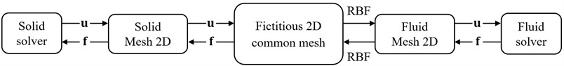
In this setup, forces and displacements are exchanged across a 2D fictitious interface mesh. The fluid solver transfers a traction vector resulting from the viscous and pressure stress to the structural solver as external loads, while the structural solver transfers the displacements back to the fluid solver. The information exchange occurs within an iterative loop until convergence is reached at each time step, according to a parallel implicit coupling scheme, where the two solvers are executed simultaneously within each coupling iteration. Mesh motion is computed using the displacement–Laplacian approach described by Eq. (4):

4

$\nabla \cdot \left(\gamma \nabla \mathbf{u}\right)=0,$

where a quadratic inverse-distance $d$ diffusivity from the fluid-structure interface, $\gamma \propto 1/d^2$, is chosen, ensuring smooth propagation of the structural displacements into the fluid domain.

The partitioned FSI coupling is stabilized and accelerated through an Interface Quasi-Newton method with Inverse Least Squares (IQN-ILS), which provides an approximation of the interface Jacobian based on the previous solutions, thus mitigating added-mass instabilities.

3. Methods

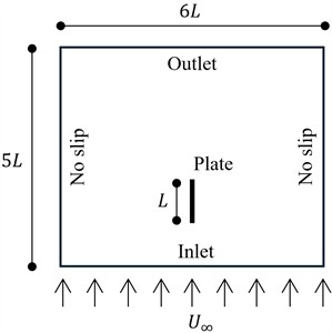
We consider a Fluid-Structure Interaction problem (see Fig. 2) of a clamped plate whose length is $L$ and thickness $h$, subjected to an incoming laminar flow having a vertical velocity $U_{\infty }$. Thickness-to-length ratio is set to $h/L=$1/40, bending rigidity, Eq. (5), is $R_1=$ 0.0125 and structure-to-fluid mass ratio, Eq. (6), is $R_2=$ 75. Reynolds number, Eq. (7), is $Re=$ 20:

where $E$ and ${\upsilon }_s$ are, respectively, Young’s modulus and Poisson’s ratio of the structural material and ${\upsilon }_f$ is the kinematic viscosity of the fluid. The computational domain has a length $5L$, a width $6L$, and a depth $L$, as shown in Fig. 2. The mesh is extended in the $X$-$Y$ plane and extruded in the $Z$ direction. It is structured and uniform, and made of hexahedral cells for both structure and fluid. A preliminary mesh convergence study (Table 1) was carried out by considering three different mesh resolutions of the fluid domain (see Fig. 7) while the Structural Mesh (SM) is always the same. Three different Fluid Meshes (FM) are analyzed: FM1, FM2 and FM3. Each mesh is obtained from the previous one through successive refinement, as shown in Fig. 7(a)-(b). The finest mesh FM3 has ${\mathrm{\Delta }x}_{FM3}=L/128$, the medium mesh FM2 has ${\mathrm{\Delta }x}_{FM2}=L/64$, and the coarsest mesh FM1 has ${\mathrm{\Delta }x}_{FM1}=L/32$. For every mesh, a time step $\mathrm{\Delta }t$ is employed to keep the Courant-Friedrichs-Lewy number, $CFL<1$, Eq. (8), ensuring both numerical stability and solution accuracy:

With regard to the IQN-ILS coupling parameters, a tolerance $e_{FSI}=$ 10^-3 was adopted for the partitioned FSI solution, with a maximum number of iterations $N_{max}=$ 300 and an Initial Relaxation Factor $IRF=$ 0.5. The mapping of forces and displacements onto the fictitious exchange mesh is performed using polynomial Radial Basis Functions with a radius $R_{RBF}=L$.

Fig. 2Computational domain and boundary conditions sketch

4. Results

The results of the numerical simulations are presented. The behavior of the plate is analyzed via the transverse, $x$, and streamwise, $y$, displacements of the plate tip, as well as the drag and lift coefficients, $C_D$ and $C_L$, defined in Eq. (9-10):

where $A$ is the surface area, $p_r$ the reference pressure, ${\mu }_f$ the fluid dynamic viscosity and ${\mathbf{R}}_d$ the deviatoric component of the Reynolds stress tensor $\mathbf{R}$. Summation on all surfaces, $A_i$, whose pressure value is $p_i$ and normal vector ${\mathbf{n}}_i$, produces the resultant forces. Convergence analysis is based on residuals associated to quantities of interest, such as $C_D$, $C_L$, $\mathbf{u}$, and computed as:

where, $∎$ represents the considered quantity, ${∎}_{pr}$ the value of $∎$ computed using the previous mesh definition and ${∎}_{ref}$ the corresponding reference value, computed, in this case, using finest mesh FM3. Fig. 3 illustrates the outcome of this study, with reference to $C_L$. Similar results are obtained for all other quantities. Based on this study of convergence, we adopt the latter mesh.

Fig. 3Residual of CL for increasing mesh resolutions

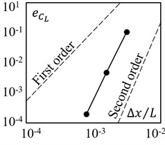
Fig. 4Phase portrait of the tip plate displacements

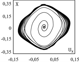
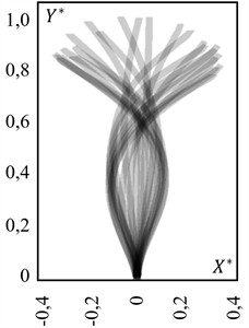
Fig. 5Motion diagram of the tip plate displacements

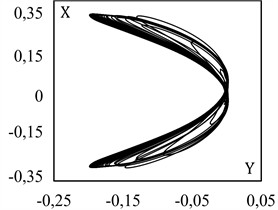
Fig. 6Time histories of drag and lift coefficients CD* and CL* respect to the flapping times of the plate. CD* is translated and aligned with the horizontal axis. The detail shows the solution for all meshes

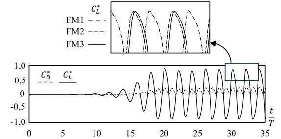
Fig. 70.2L×0.2L mesh box detail for the plate tip

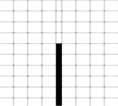
a) Mesh FM1

b) Mesh FM3

Under the assumed set of parameters, the thin plate under study reaches a stable flapping regime after approximately 25 flapping cycles, as indicated in Fig. 6, showing the flapping time-dependent behavior of the dimensionless drag and lift coefficients, respectively $C_D^{*}=C_D/C_{D,max}$ and $C_L^{*}=C_L/C_{L,max}$. Fig. 4 presents a phase portrait, the normalized transverse tip velocity of the plate, $U_x=V_x/U_{\infty }$, is plotted against the normalized transverse tip displacement, $X^{*}=x/L$. In Fig. 5 is shown the tip plate track in the $X$-$Y$ plane. Fig. 8 shows the Fast Fourier Transform (FFT) of the displacement amplitude in the frequency domain for FM3 mesh. Finally, Fig. 9 shows the envelope of the deformed configurations of the plate over one flapping period $T$, reporting the normalized displacements $X^{*}=x/L$ and $Y^{*}=y/L$.

Fig. 8Fast Fourier Transform in the frequency domain of the plate tip for mesh FM3

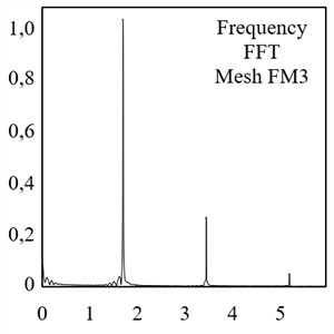
Fig. 9Normalized displacement envelope during a flapping period T

5. Conclusions

This study presents selected results from ongoing research into the development of a fully open-source framework for analysing the interaction between fluids and highly flexible structures. A dynamic analysis of a thin plate subjected to FIV was performed in limit-cycle oscillation conditions. This allowed to characterise the spatiotemporal evolution of the flow field, and its correlation with the aerodynamic lift and drag coefficients. The present results are intended as a first numerical assessment of the framework, while quantitative validation against literature data for analogous configurations will be addressed in future work. Further work also will focus on investigating the potential of this approach for high fidelity engineering applications.