Experimental study on vibration characteristics of fluid-solid coupling cantilever thin aluminum plate

1. Introduction

The modal analysis technology originated in the 1930s and was first applied to the measurement of aircraft modal parameters in the aviation field. After decades of development, especially the maturity of sensor technology, modal analysis has developed rapidly, which has become an important part of the field of vibration engineering [1]. The structure cannot exist independently from the fluid environment. According to the influence of fluid, the modal analysis can be divided into two types: dry modal analysis and wet modal analysis. Dry modal analysis generally ignores the effects of light fluids, and the default structure is calculated in a vacuum environment. The wet mode problem must consider the influence of the additional fluid on the vibration characteristics of the structure. For the small deformation problem, to simplify the calculation, the fluid can be applied to the structure as an additional mass for analysis [2, 3]. The interaction between fluid and structure is a fluid-solid coupling problem [4].

Fluid-solid coupling phenomena are widely found in aerospace, marine, pressure vessels, rail transit, etc. For example, the response of marine pipelines excited by internal and external fluids [5, 6]. Interaction between a high-speed turbine and a high-speed flowing gas or water stream [7, 8]. The attitude of the train running under the action of aerodynamic force [9], etc. Furthermore, the experimental and numerical modal analysis conducted in Ref. [2, 10, 11] suggested that the coupling between the structure and fluid causes the structure to be affected by the fluid in terms of added mass distribution, damping force and elastic restoring force, and thus the vibration characteristics of the structure are changed. Therefore, the fluid-solid coupling vibration problem under the action of fluid is much more complicated than the vibration in the air. In order to reduce the difficulty of analysis, complex engineering problems are usually simplified, the most critical of which is to select key parts of the system and abstract the simplified model for research [12]. The elastic thin plate is one of the most common simplified models, such as turbine blades, water tanks, and thin-walled structures on equipment casings that can be simplified to elastic sheet problems [13-19]. For the fluid-solid coupling problem of elastic thin plates, the research mainly focuses on the numerical analysis of dynamic and static problems of coupled systems [15, 20-22]. In the study of the description of the deformable plate and fluid interaction, the compatible Lagrangian-Eulerian method can be used. When the solid deformation is small, the problem can be further simplified, but it is insufficient in describing the contact conditions. It is not suitable for cases where the shape of the plate and the flow range vary greatly. For complex problems, the arbitrary Lagrangian-Eulerian method can be used to describe the motion interface continuously and accurately, the method can continuously and accurately track the motion interface and maintain a good unit shape, and it is easy to realize the transformation to Lagrangian coordinates. For fluids and elastomers, it is easy to achieve interface transitions to ensure compatibility and coordination [23]. The experimental modal analysis can take into account the actual factors in engineering practice and obtain real and reliable results. However, the cost of underwater testing is high, and the performance requirements of waterproofing and electrical insulation are proposed for the sensor. Therefore, the underwater vibration test is often difficult to develop due to the limitation of objective conditions. In general engineering, in order to quickly obtain the underwater natural frequency of the structure, it can be obtained by multiplying the natural frequency of the structure in the air by an empirical influence coefficient. Different structures have different empirical coefficients, so the appropriate means to explore the modal measurement of underwater structures has become one of the research hotspots. The experimental methods of modal analysis mainly include the acceleration sensor method, laser Doppler vibration measurement method [13, 16], etc. The former requires a large number of wiring and bonding sensors, the influence of additional quality can’t be ignored. Laser Doppler is limited to point-by-point measurement, and it must take a lot of time to get the full-field mode.

The modern photometric method has the advantages of full field, non-contact, high precision, and has been widely used in engineering measurement [24-26]. In this paper, the physical model of the cantilever elastic plate under the simplified fluid-solid coupling is established. Electronic speckle interferometry was employed as an experimental measurement method to study the modal characteristics of cantilever aluminum in air and fluid environment. The effects of fluid additional mass, additional damping, pressure and other factors on the vibration mode and natural frequency of the structure, as well as the relationship between the size of the coupling interface and the natural frequency of the structure, are discussed. At the same time, the equivalent finite element model is established by using the wet modal analysis module in the commercial software ANSYS Workbench. The calculated results agree well with the experiment.

2. Experimental procedure

2.2. Time average real-time image subtraction

Since the vibration mode image obtained by the time-averaging method is affected by the random phase difference (i.e. speckle) and the direct object light and reference light intensity, the actual experimental results cannot be used for modal analysis. Due to the interference of the measurement environment and the disturbance of the airflow, the time-average image gradation Eq. (4) collected by the CCD camera at different times includes a random phase difference $\varphi (x,y)$ of the spatial distribution related to the object beam and the reference beam, and There is a time-dependent random phase caused by the above factors, at the same time, there is also a time-dependent random phase caused by the above factors [28]. Let this time-dependent random phase size be $\delta \left(t\right)$, For the case of the Eq. (4), it is equivalent to $\delta \left(t\right)=0$ at this time. For the sake of brevity, when the sample is in a vibrating state, in the two time-average images acquired by the CCD camera at different times, the time-dependent random phase size of one image is $\delta \left(t\right)$, and the size of the other is 0. Then the real-time subtraction result of the two images can be abbreviated as the following expression [30]:

5

$g\left(x,y,t\right)=4\sqrt{I_O{I}_R}\left|\mathrm{s}\mathrm{i}\mathrm{n}\left[\varphi \left(x,y\right)+\frac{\delta \left(t\right)}{2}\right]\mathrm{s}\mathrm{i}\mathrm{n}\frac{\delta \left(t\right)}{2}{J}_0\left(m\right)\right|,$

where $\sin \left[\varphi \left(x,y\right)+\frac{\delta \left(t\right)}{2}\right]$ still represents a random speckle term; $\sin \left[\frac{\delta \left(t\right)}{2}\right]$ modulates the grayscale of the overall image, affects the contrast of the fringes.

Fig. 1Schematic of out of plane movement detection system

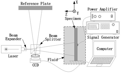
Fig. 2Variation of gray-value with vibrating amplitude: a) zero-order Bessel function, b) first-order bending fringe pattern of cantilever beam, c) first-order bending mode of cantilever beam

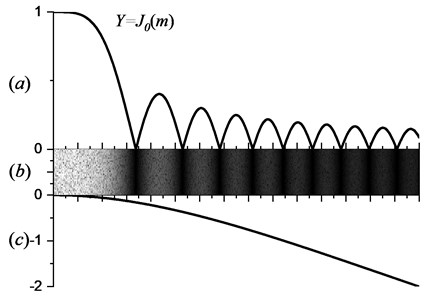
As shown in Fig. 2(a) is a zero-order Bessel function, Fig. 2(c) is a first-order bending mode of the cantilever beam, and Fig. 2(b) is a modal fringe pattern corresponding to the first-order bending mode of the cantilever beam. It can be seen from Fig. 2 that the image gray value corresponding to the vibration nodal line region is the largest.

2.4. Experimental device and experimental model

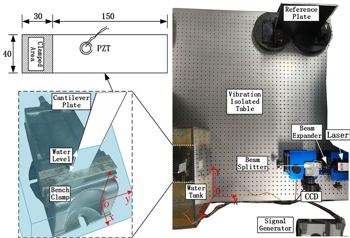
In order to study the modal characteristics of the thin plate under fluid-solid coupling, a fluid-solid coupling modal experimental system of cantilever aluminum plate as shown in Fig. 3 was built on the isolation platform. The system consists of three parts: electronic speckle interferometric modal measurement optical path, excitation system and fluid-solid coupling device. The test piece is made of aluminum alloy plate with a thickness of 2 mm and is cut into two rectangular plates of 180 mm×40 mm by wire cutting. One end is clamped and fixed by a vise to form a cantilever plate, and placed in a transparent water tank with a 400 mm×600 mm horizontal section. The specimen cantilever size is 150 mm×40 mm×2 mm, the material parameters are elastic modulus $E=$7.1×10¹⁰ Pa, Poisson’s ratio $\nu =$0.33, density $\rho =$2.77×10³ kg/m³. The test piece is excited by a circular lightweight thin piezoelectric ceramic piece (PZT) attached to the backside. The piezoelectric ceramic piece has a diameter of 15 mm and a thickness of 0.4 mm. The surface of the piezoelectric ceramics and the solder joints are fully waterproofed, and the excitation points are avoided as far as possible from the pitch line position. In the measurement system shown in Fig. 3, the power of 80 lasers produces a green coherent laser with a wavelength of 532 nm; the CCD is a 1280×1024 pixel programmable control camera from IDS, Germany; the signal generator can generate a 0-25 MHz sine wave made by the RIGOL, China.

In the case of no water, the excitation frequency is slowly adjusted, and the actual resonance frequency is accurately located by the aforementioned amplitude fluctuation resonance discrimination method. Then, Keep the frequency unchanged, the time average real-time image subtraction method is used to obtain natural frequencies and modal fringes of the first 13 orders of the cantilever aluminum plate in air. Then, water was added to the water tank in stages, and the water depth increased by 5 mm each time. The results of 14 sets of working conditions are obtained by the same measurement method. The experimental ambient temperature is 25 degrees Celsius.

Fig. 3Experimental setup and model

2.5. Acoustic-solid coupling finite element method

When the solid structure vibrates and deforms in water, the surrounding water body also moves synchronously. Therefore, the influence of external water on the structure needs to be considered in the structural vibration problem. The coupling of structure and fluid in the vibration process is the fluid-solid coupling problem. The interaction between two-phase media is a distinct feature of fluid-solid coupling. Deformed solids can deform or move under fluid loading; deformation or motion, in turn, affects fluid motion, thereby changing the distribution and size of fluid loads. The research methods of fluid-solid coupling mainly include two methods: cross-iteration, direct simultaneous solution, and finite element solution. The acoustic-solid coupling method used in this paper is one of the finite element methods. For the "wet" mode extraction problem of the structure, the traditional method is to calculate the quality of the attached water as an additional mass point on the propeller model, so that the workload is large, and the weight of each small area of the three-dimensional structure needs to be Manually added, while the interaction between water and structure cannot be considered. The commercial software ANSYS Workbench provides an acoustic unit to simulate this type of problem, which can be used to simulate the weight, pressure and adhesion of the surrounding wet surface and attached water. Therefore, this paper chooses the acoustic fluid-solid coupling method to approximate the simulated fluid-solid coupling problem.

The finite element method is one of the most widely used numerical methods for solving fluid-structure interaction problems. The solution is to divide the computational model into finite elements, and then construct a simple field function with only a finite number of parameters to be determined for each unit. The set of field functions can represent the field function of the whole continuum. Finally, a set of algebraic equations with a finite number of parameters to be determined can be established according to the energy equation or the weighted residual equation. The numerical solution of the finite element method is obtained by solving the discrete equations.

When the action of the fluid is not considered, the structural dynamics equation of the discretized structural model with n degrees of freedom can be expressed as:

9

$M_s\ddot{u}+C_s\dot{u}+K_{s}u=F_s,$

where $M_s$ is the mass matrix of the system, $C_s$ is the damping matrix of the system, $K_s$ is the stiffness matrix of the system, $\mu$ is the displacement vector of the node, and $F_s$ is the exciting force of the system.

When the structure is in a static fluid, some assumptions are made about the equation considering the fluid-solid coupling: the fluid is compressible, the pressure fluctuations will cause a change in density; the fluid is non-viscous and non-rotating; the fluid has no motion. Therefore, the fluid will be treated as an acoustic fluid and the governing equations can be expressed by the following acoustic equations:

10

$\frac{1}{c^2}\frac{{\partial }^{2}p}{\partial t^2}-\mathrm{\Delta }p=0,\mathrm{}\mathrm{}\mathrm{}\mathrm{}\mathrm{}c={\left(\frac{k}{{\rho }_0}\right)}^{\frac{1}{2}},$

where $c$ is the velocity of sound propagation in water, $p$ is the pressure of the color fluid caused by sound waves and the force acting on the fluid, $∆$ is the Laplacian operator, $\mathrm{k}$ is the fluid volume modulus, and ${\rho }_0$ is the average density of the fluid. At the fluid-solid coupling interface, the following equations can be used to describe the interaction of fluids and structures:

11

$n\cdot \nabla p=-{\rho }_{0}n\cdot \ddot{u},$

where, $n$ is the unit normal vector at the interface and $\nabla p$ is the pressure gradient along the normal vector. Therefore, Eq. (10) can be discretized as:

12

$M_f\ddot{p}+C_f\dot{p}+K_{f}p+M_{sf}\ddot{u}=0,$

where $M_f$ is the fluid equivalent mass matrix, $C_f$ is the fluid equivalent damping matrix, $K_f$ is the fluid equivalent stiffness matrix, and $M_{sf}$ is the equivalent coupling mass matrix acting on the fluid. Considering the effect of water pressure on the structure at the interface, Eq. (9) is rewritten as:

13

$M_s\ddot{u}+C_s\dot{u}+K_{s}u+K_{sf}p=F_s.$

Therefore, the modal solution equation considering fluid-solid coupling is as follows:

14

$\left[\begin{array}{cc}{M}_s& 0\\ M_{sf}& M_f\end{array}\right]\left\{\begin{array}{l}\ddot{u}\\ \ddot{p}\end{array}\right\}+\left[\begin{array}{cc}{C}_s& 0\\ 0& C_f\end{array}\right]\left\{\begin{array}{l}\dot{u}\\ \dot{p}\end{array}\right\}+\left[\begin{array}{cc}{K}_s& K_{fs}\\ 0& K_f\end{array}\right]\left\{\begin{array}{l}u\\ p\end{array}\right\}=\left\{\begin{array}{l}{F}_s\\ 0\end{array}\right\}.$

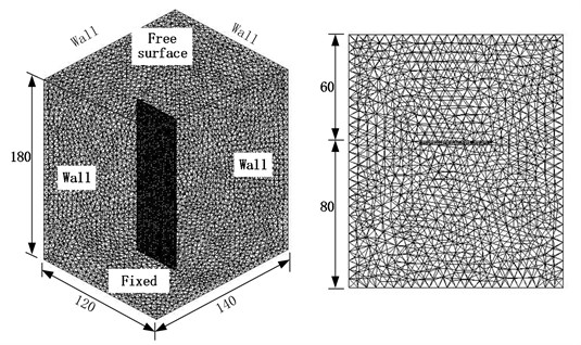
Based on the commercial finite element software ANSYS workbench, the modal characteristics of the cantilever aluminum plate in air and water are numerically calculated. For the modal calculation of the aluminum plate in the air, the influence of the fluid can be neglected, and the dry mode calculation can be directly performed. For the modal calculation of structures in fluids, a three-dimensional model of the fluid-solid coupling field equivalent to the experimental one is required. The model consists of two parts, water and cantilever aluminum plate. Since the actual water tank is much larger than the structure, considering the limitation of the calculation amount, the flow field area is set to a rectangular parallelepiped of 120 mm×140 mm×180 mm, The size in both directions of the horizontal plane is more than twice the size of the structure, and the vertical direction is the same as the actual situation, which can be considered to have good equivalence with the experiment. The equivalent model is meshed by the software’s own modeling tool. The structure part adopts a hexahedral mesh, and the fluid adopts a tetrahedral mesh. Among them, the structure is the key point of calculation, the grid needs to be encrypted, the grid size of the cantilever plate is set to 1 mm, and the grid of the fluid area is 5 mm, as shown in Fig. 4 is the fluid-solid coupling finite element model. According to the experimental conditions, the parameters of the finite element model are set: the low end of the cantilever plate is a fixed constraint, the boundary of the fluid domain was show in Fig. 4 the material parameter is aluminum alloy, the fluid model is defined as acoustic fluid, the material is water, the sound velocity is 1.5 km/s, and the gravity acceleration is 9.8 m/s². The contact surface is defined as the fluid-solid coupling surface, such that the structure is subjected to a force loading due to the fluid pressure along with the fluid-structure interface, and at the same time, the pressure field in the fluid is affected by the motion of the elastic structural boundary.

Fig. 4Fluid-structure coupled finite element model

3. Experimental results and discussion

The first eleven modes were alternated by pure bending and combined bending and torsion modes which can be compared in both shape and frequency sufficiently, and the two high order torsion modes observed subsequently were used to studied difference in shape of numerical and experimental results, so one gives first 13 order modes of the cantilever aluminum obtained by experiment and simulation based on above consideration. Table 1 shows the first 13 modes of the cantilever aluminum plate in air. The experimental frequency takes the average of two cantilever aluminum plates. The experimental mode and finite element calculation results are basically the same, and the frequency error is less than 2 %, indicating that the electronic speckle test method has good reliability and accuracy. As described in the theory, the fringe pattern is modulated by a zero-order Bessel function. The brightest line in the figure represents the node line of the mode, and its amplitude is zero. By the position of the node line, the mode shape of the board can be divided into: Pure bending vibration, pure torsional vibration and combined bending and torsional vibration. Due to the small out-of-plane stiffness of the cantilever thin plate structure and the large lateral stiffness, the first 13 modes are mainly bending vibration and low-order bending and torsion combined vibration modes, among which the 1st, 2nd, 4th, 6th and 8th, 10th is a pure bending mode, 3rd and 12th are pure torsional vibration modes, and 5th, 7th, 9th, 11th and 13th are combined bending and torsion modes.

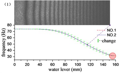
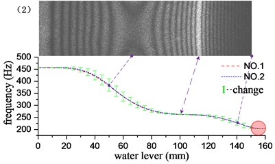
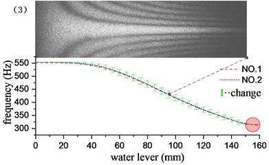
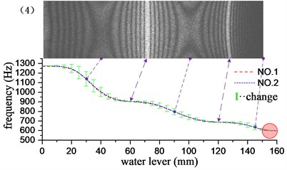
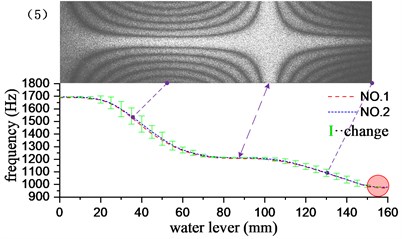
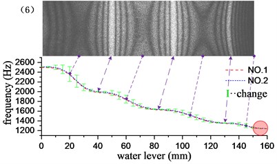
Through the underwater test modal analysis, the actual factors in the engineering practice can be considered, and the vibration characteristics of the underwater structure can be obtained. To explore the influence of the size of the acoustic solid contact surface on the vibration characteristics of the structure, the experimental design of different water level heights as a control, slowly graded water into the water tank, each water level increased by 5 mm, each group of experiments recorded the frequency and vibration of the structure according to the aforementioned experimental method. It is found through experiments that when the water is about to reach and has not passed the cantilever plate, the frequency change is very small. Therefore, the experimental group reaches the water level beyond the height of the cantilever plate by 10 mm, and it can be considered that the vibration characteristics tend to be stable. The water level-frequency curve is obtained by stepwise adding water, and the experimental results corresponding to the first 6 order mode are given in Fig. 5. The short vertical line in the figure is the difference between the adjacent two levels of water depth corresponding to the modal frequency of the cantilever aluminum plate, and the length of the vertical line reflects the speed of the frequency drop. It can be seen from the variation in the figure that the change of the frequency is related to the amplitude of the cantilever plate where the liquid level is located, and the frequency change value increases with the increase of the amplitude, and decreases with the decrease of the amplitude, at the position of the node line, the rate of change of frequency is close to zero. However, this relationship is not an exact correspondence. The frequency change has a certain degree of advancement with respect to the amplitude: the longest vertical line appears before the maximum amplitude point, and the shortest vertical line appears before the node line point. This phenomenon may be caused by additional mass distributed unevenly. Because the structure is a continuum, the additional mass and additional damping of the uneven distribution not only affect the structure of the contact surface, but also affect the structure surface disconnected. It has a greater impact on the structure near the interface, and the effect on the structure far from the interface is gradually reduced. As the modal order increases, the structural radiation area influenced by the additional mass matrix and damping matrix is gradually reduced. For example, in the first-order bending vibration, the point of the fastest frequency change is 40 mm ahead of the point of maximum amplitude. In the 4th order bending vibration, the corresponding value is 10 mm.

Table 1The first 13 modes of the cantilever aluminum plate in the air

Ord	1	2	3	4	5	6	7	8	9	10	11	12	13
Exp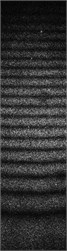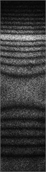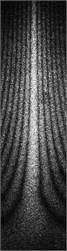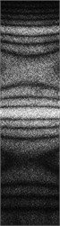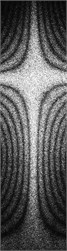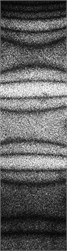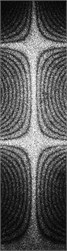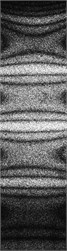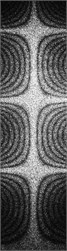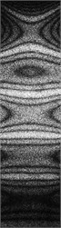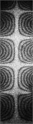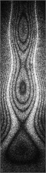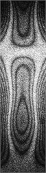
Fre/Hz	73.9	455.8	551	1270.6	1689	2496.7	2969.2	4138	4498	6142	6311	7027	7807
FEM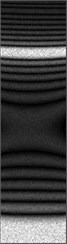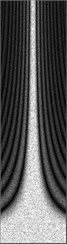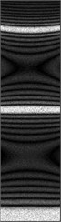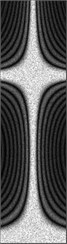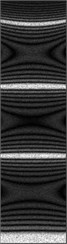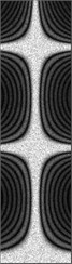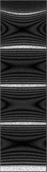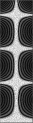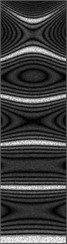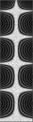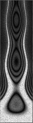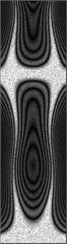
Fre/Hz	73.6	460.1	550.58	1290	1705	2532.1	3010.4	4186	4545.7	6215.7	6371.3	6818.5	7486.7
Err/%	–0.38	0.95	–0.08	1.53	0.95	1.42	1.39	1.16	1.06	1.2	0.96	–2.97	–4.1

As shown in the red circle area in Fig. 5, when the water level depth exceeds the cantilever plate, the modal frequencies of the various stages tend to be stable, and the frequency remains basically unchanged when the water level continues to rise. At this time, the additional mass and the additional damping are evenly distributed in the whole field position of the structure, and the vibration characteristics of the structure do not change substantially with the increase of the water level, which indicates that the additional mass and additional damping generated by the fluid are the main factors causing the structural vibration characteristics to change, nevertheless, fluid pressure has little effect on structural vibration characteristics. The first 13 order modal results of the cantilever aluminum plate obtained by the experimental method and the acoustic-solid coupling finite element method are shown in Table 2, respectively. Compare finite element calculations and experimental results, the modal vibration modes are basically the same, and the frequency difference is mostly within 2 %, This proof that the test method and the finite element model are reliable and accurate. The finite element model does not take into account the additional effects of piezo ceramic exciters, wires, and waterproof materials, which may result in some orders of difference in results exceeding 3 %, such as the 1st and 12th modes.

Fig. 5Influence of different water levels on the first 6 natural frequencies of cantilever plates

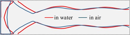
The additional mass and damping obviously affect the natural frequency and response amplitude of the structure. For the same response amplitude, the underwater mode requires a larger excitation voltage. For some modalities, even if the maximum voltage is applied, only a weak response amplitude can be produced, such as the 11th order mode under water. The additional mass and damping have little effect on the low-order vibration modes of the structure. The comparison shows that the first 11 order modes of the air and the underwater are basically the same, while for the higher-order modes, the additional mass and damping have a significant influence on the mode. As shown in Fig. 6, Fig. 6(a) is a comparison of the 12th order modal line in underwater and air. It can be found that there is a slight deviation in the position of the node line. Fig. 6(b) is a comparison of the 13th order mode line in the air and under the water. It can be seen that there is a significant deviation between the two line positions.

Table 2The first 13 modes of the cantilever aluminum plate in water

Ord	1	2	3	4	5	6	7	8	9	10	11	12	13
Exp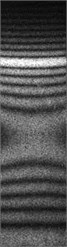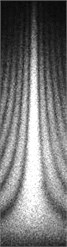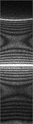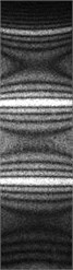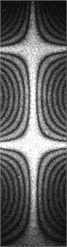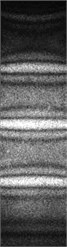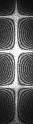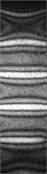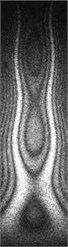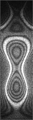
Fre/Hz	31.5	202.7	313.4	597.6	973	1238.2	1740	2148	2701	3363	3875	4559	4918
FEM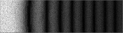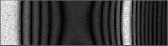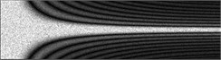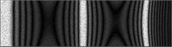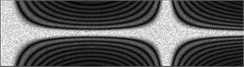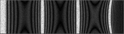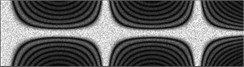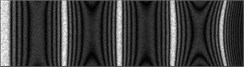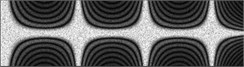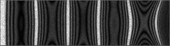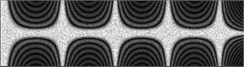
Fre/Hz	30.5	199.1	306.5	592.0	960.5	1236.9	1729.6	2162.5	2671.9	3381,2	3833.6	4333.7	4767
Err/%	–3.14	–1.79	–2.21	–0.94	1.28	–0.01	–0.6	0.68	–1.08	0.54	–1.07	–4.9	–3.07

Fig. 6Comparison of modal nodal lines in underwater and air: a) 12th order, b) 13th order

a)

b)

Fig. 7 shows the first 13 natural frequencies of the cantilever aluminum plate completely in air and completely in water. It can be seen that the natural frequency of the cantilever aluminum plate measured in water is greatly reduced. The degrees of decline are between 35 % and 55 %. And the frequency decline trend is related to the mode shape: for each mode of the pure bending mode, the frequency change rate is linear, linear fitting of each point can be used to obtain a linear equation: $w=$ 1.3109$n-$58.375; For each mode of the combined mode with the first-order torsion, the frequency change rate shows another linear distribution, and the linear fitting results in $w=$0.5743$n-$45.112. At the same time, the frequency drop rate of the pure bending mode is generally lower than that of the combined bending and torsion mode. As the modal order increases, the rate of change of each mode gradually becomes smaller, and the two fitted lines gradually approach. It can be predicted that when it is at a higher mode, the two will tend to intersect.

Fig. 7Comparison of the first 13th order wet and dry modal frequencies of cantilever plate

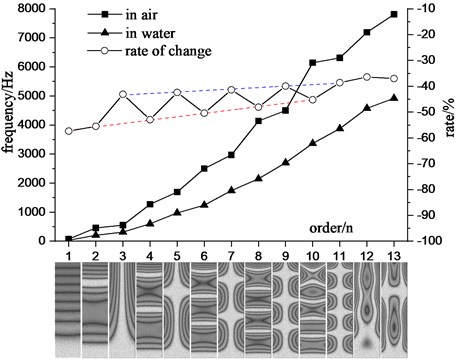
In more complex engineering applications, it is often easier to measure the low-order modes of the structure, and it is difficult to measure the higher-order modes. It can be seen from Fig. 7 that for all bending modes, and the combined mode with the first-order torsion, their frequency changes show good linear characteristics. Therefore, high frequency can be predicted by measuring a small amount of low frequency during the experiment to reduce the workload and measurement difficulty.

4. Conclusions

Based on the electronic speckle interferometry method and the acoustic-solid coupling finite element numerical simulation, the dry and wet modal characteristics of the cantilever aluminum plate under fluid-solid coupling are studied. The resonance frequency and modal fringe pattern of the cantilever aluminum plate under different working conditions are obtained accurately by the amplitude fluctuation resonance discrimination method. Since the results are in good agreement with the finite element method, the reliability and accuracy of the experimental model and the finite element model established in this paper can be proved. According to the analysis of the experimental results, the following conclusions can be drawn:

1) The action of the fluid will greatly reduce the natural frequency of the structure, and the frequency of each order drops between 35 % and 55 %. The effect of the fluid on the low-order mode has little effect, but the effect for higher-order mode is more obvious. The main cause of the change in structural vibration characteristics is the additional mass and additional damping produced by the fluid, while the additional pressure has a weak effect on the structural vibration characteristics.

2) With the gradual increase of the fluid-solid coupling interface, the rate of decline of the natural frequency and the amplitude at the gas-liquid interface are correlated. The rate of decline fluctuates with fluctuations in amplitude and slightly ahead of the amplitude characteristics. Due to the continuity of the structure, the additional mass and additional damping have a radiating effect on the non-fluid contact area of the structure, and as the order is gradually increased, the effect of the radiation is gradually reduced.

3) For each mode with the same characteristics, the frequency decline trend is linear. For example, the pure bending vibration modes have a linear relationship of frequency reduction rate: $w=$ 1.3109$n-$ 58.375; The combined vibration mode with the first-order torsion has a linear relationship of frequency reduction rate: $w=$ 0.5743$n-$45.112.

4) In the actual engineering problems, it is difficult to measure the high-order frequency of the structure. According to the linear relationship of the same type of mode described in the conclusion of Article 3, the fundamental frequency of the structure can be accurately measured to reasonably predict the high frequency of the structure to reduce the test workload.