Abstract
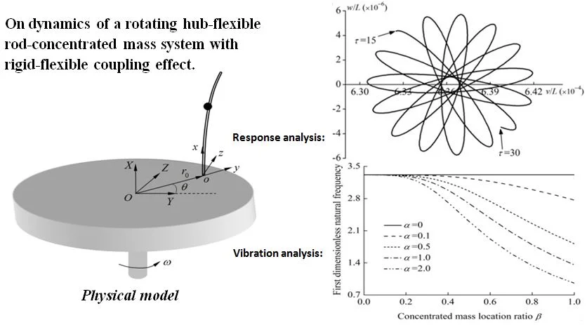
Rotating hub-flexible rod system is a typical rigid-flexible coupling dynamic mechanism, which has a wide range of industrial applications. In this paper, a comprehensive nonlinear dynamical model of a rotating hub-flexible rod-concentrated mass system considering rigid-flexible coupling effect is established to study its dynamic properties. By employing the Hamilton principle and classical beam theory, a set of differential equations of motion are derived including the couplings of the elastic deformation of the rod and the rigid rotation of the hub. The additional centrifugal force, tangential force and Coriolis force due to the rigid-flexible coupling effect are elaborated. The derived governing partial differential equations are solved by the Galerkin method. The validity of the present model is verified by a comparative study. The tip motion trajectories of the rod for the prescribed rotation, the dynamic responses of the hub and the rod for an external torque acting on the hub and the dimensionless natural frequencies of the system for the steady-state rotation are graphically presented. The influences of parameters such as rotational speed ratio, concentrated mass ratio, concentrated mass location ratio and initial eccentricity ratio on the dynamics are discussed in detail.
Highlights
- A dynamic model of a rotating hub-flexible rod-concentrated mass system is developed.
- The mechanism of rigid-flexible coupling effect is expounded.
- The centrifugal, tangential and Coriolis effects on the tip motion trajectories are discussed.
- The influences of related parameters on the dynamics and vibrations are studied.
1. Introduction
The dynamic problems (such as transient response and free vibration) of rotating flexible beams (rods) are the key research topics in a lot of engineering applications such as aerospace, robotics, propellers, turbine blades etc., which are crucial for design purposes, optimization and control. The study on the dynamic behavior and stability of these structures is an essential part of the design process, especially when dealing with the design of control and condition monitoring systems. Rotating beam (rod) structures generally include both the small elastic deflections of the flexible beam and the overall rotating motion of the hub, which are referred to the rigid-flexible coupling mechanisms. The rotating hub-flexible rod presented herein is a typical example. Therefore, more reliable mechanical models and their solution strategies for these coupling mechanisms have been required for accurate speed control and accurate operation [1-3].
The dynamic modeling of the rotating hub-beam (rod) structure has roughly gone through three stages. The dynamic model of the first stage was known as the traditional hybrid coordinate model [4-8], in which the small deformation hypothesis of the traditional structural dynamics was applied. It is assumed that the axial and lateral deformations of the beam were not coupled to each other. This model was generally used in the case that the large overall motion was known. In this case, only the influence of the overall motion of the hub on the elastic deformation of the rod was discussed while ignoring the influence of the flexible deformation of the rod on the rigid overall motions.
The dynamic models of the second stage were called the dynamic stiffening models, in which the dynamic stiffening effect was first proposed by Kane et al. [5] in 1987. It was demonstrated that the traditional hybrid coordinate model failed to handle the dynamics of rotary hub-rod system with high angular velocity. Thereafter, many models were established to capture the dynamic stiffening effect, which can be roughly divided into three categories. The dynamic stiffening models of the first category added the additional potential energy induced by centrifugal force to describe the centrifugal stiffening effect [9-14]. In the second type of dynamic stiffening models [15-22], the axial deformation is described by using the stretch deformation (i.e. a non-Cartesian variable) and taking into account the second-order coupling deformation caused by the transverse deformation. The dynamic stiffening models of the third category used a geometrically exact approach to describe the centrifugal stiffening effect [23-26]. Although the introduction of dynamic stiffening enables the dynamic model to deal with the dynamics of high-speed rotating beam systems, there are still limitations on understanding of the rigid-flexible coupling mechanism of such systems.
The dynamic model of the third stage is the rigid-flexible coupling model (RFC model) [27], which is developed through the classical continuum mechanics. The RCF model considers that the essence of the dynamic stiffening effect is the structural dynamics of the non-inertial system. The coupling effect of the large overall motion of the rigid body and the elastic deformation of the beam results in the additional stiffness, which leads to the dynamic stiffness of the system. Liu and Hong [28] investigated the dynamic stiffening effect on the dynamic behaviors of a elastic slender beam undergoing free overall motions based on the rigid-flexible coupling theory. Cai et al. [29] developed the first-order approximation coupling (FOAC) model for rotary hub-beam-tip mass system and investigated its dynamics of the system when the rotation motion was unknown. Based on the Timoshenko beam theory, You et al. [30] proposed the dynamic model of a rotary flexible hub-beam system and studied the influence of the transverse shear deformation on the dynamic behaviors. On the basis of a new rigid-flexible coupling dynamical model, Li and Zhang [31] investigated the dynamic responses and free vibrations of rotary tapered beams made of axially functionally graded materials by utilizing the B-spline approach. Liu et al. [32] presented a rigid-flexible coupling dynamic model for a rotary rigid body-flexible rod-tip mass system. Since the mass of the flexible rod was neglected, the model presented by Liu et al. [32] was actually a two-degree-of-freedom model. Recently, by utilizing the slope angle of the beam, Zhang et al. [33] developed a new rigid-flexible coupling dynamical model of a rotary hub-flexible beam-tip mass system under gravity loads, and determined the natural frequencies and nonlinear frequency responses through the incremental harmonic balance method.
In this study, a rigid-flexible coupling dynamical model of a rotary hub-flexible rod-movable concentrated mass system is developed by employing Hamilton’s principle. Based on the accurate geometric nonlinearity, the second-order coupling deformations caused by the transverse deformations are employed to capture the dynamic stiffening effect. The derived partial differential governing equations are solved numerically by the Galerkin method. A comparative study is carried out to verify the present model. The dynamic responses of the system for situations of a prescribed rotation and an arbitrary external torque acting on the hub are presented. The influences of rotational speed ratio, concentrated mass location ratio, concentrated mass ratio and initial eccentricity ratio on the responses are studied. Finally, the natural frequencies of the rotating flexible rod under steady-state rotation are calculated.
2. Nonlinear dynamic modeling of the system
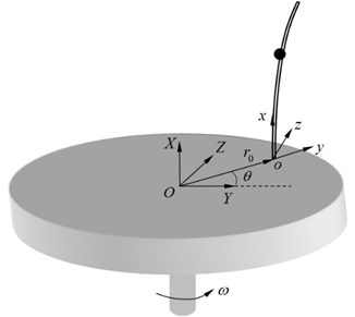
Fig. 1 shows a rotating hub-flexible rod-concentrated mass system. The flexible rod with length , cross-sectional area , mass density , Young’s modulus , is attached to the rigid hub, which rotates about the fixed vertical axis (i.e., -axis). Parameters and are the rotary inertia and rotation angle of the hub with respect to -axis. The - is the inertial reference frame, whereas the - is the floating one that is fixed on the rod. In the present study, a concentrated mass considered can be moved along the centroid axis of the rod.
Since a slender rod is considered herein, the classical beam theory is used to describe its deformations. The deformation field of a generic point on the deformed rod with respect to the floating reference frame can be expressed by:
where , and are the deformation components at the centroid axis along -, - and - directions, respectively.
Fig. 1A rotating hub-flexible rod-mass system
Based on the relation of the geometric nonlinearity, the axial deformation could be described by using the arc-length and the transverse deformations, as [16, 21]:
in which the terms of and are called as the non-linear second-order coupling deformations.
Based on the von Kármán strain theory, the axial normal strain is given by:
Utilizing the uniaxial stress-strain relations, the corresponding normal stress is:
Without considering the effect of gravity, the potential energy of the system can be written by:
where and are the cross section moments of inertia with respect to and axes, respectively.
The position vector of the point in the inertial reference frame can be written by:
in which, is the rotation transformation matrix. is the position vector of the point in the inertial frame. is the position vector of the point on the undeformed rod in the floating frame. The matrix , the vectors and are given by:
Accordingly, the absolute velocity of the point can be derived by:
where is the rotational speed. The matrix can be expressed by:
Therefore, the kinetic energy of the system is:
An external rotating torque is assumed to act on the hub and thus external virtual work is derived by:
where and are the external distributed forces acted on the rod along the and directions.
The rigid-flexible coupling dynamic equations of the rotating hub-flexible rod system are derived by the following Hamilton’s principle, as:
Substituting Eqs. (5), (10) and (11) into Eq. (12), one can obtain the comprehensive nonlinear differential equations of the system:
where .
The corresponding boundary conditions of the rod are give by:
– Geometric boundary conditions: at .
– Force boundary conditions: at .
It is seen from Eq. (13) that rigid rotation of the hub and the elastic deformation of the slender rod are coupled with each other. This is referred to the rigid-flexible coupling effect, which leads to the strong nonlinearity of the system. In the rest of the present study, the axial motion of the rod is neglected since it is not coupled with the radial motion and tangential motion of the rod and the rotation of the hub.
Then, a Dirac’s delta function is applied to take into account a movable concentrated mass on the rod, as follows:
where is the distance from the mass to the root of the rod. The values of the Dirac’s delta function are given by:
Using instead of , one can rewrite the Eqs. 13(a), 13(c) and 13(d), as:
The terms of and in Eqs. (16b) and (16c) represent the Coriolis effect of the rotating rod. The centrifugal stiffening effect of the rotating rod is reflected by the terms of and . The terms of and represent the tangential effect. The terms of and in right hand of the Eqs. (16b) and (16c) are, respectively, the centrifugal force and tangential force. Obviously, both centrifugal and tangential forces depend on the rotation of the hub and the initial eccentricity of the rod (i.e. ).
The Galerkin method is employed to solve the Eq. (16) numerically, hence the deformations of and are approximately given by:
where is the number of terms of the trial functions. and denote the time-dependent generalized coordinates of the radial and tangential deformations, respectively. and are the trial functions satisfying both the natural and essential boundary conditions. In the present investigation, the transverse bending mode functions of a stationary cantilever Euler-Bernoulli beam are chosen as the trial functions, as:
where is th root of:
Before applying the Galerkin method to discrete the obtained governing equations, the variational equations of motion should be derived by multiplying Eq. (16b) and (16c) by corresponding weighting functions for the radial and tangential deformations, as:
where and are the arbitrary time-dependent functions. Applying integration by parts to Eqs. 16(c) and 16(d) over length , the variational equations can be rewritten by:
Within the process of presentation of the numerical results, dimensionless analysis is preferable. To this end, the following dimensionless parameters are defined:
where , , , , and represent the initial eccentricity ratio, concentrated mass ratio, concentrated mass location ratio, rotational speed ratio, external torque ratio and rotary inertia of the hub, respectively. Moreover, is fixed to be used.
By using the above dimensionless parameters, the discretized governing equations of motion can be written in a dimensionless matrix form:
where , and represent the generalized mass, Coriolis and stiffness matrices, respectively. and are the generalized force and coordinate arrays, respectively:
in which the elements in the sub-matrices , , and () are given by:
If the rotation of the hub is prescribed, the influence of the elastic motion of the rod on the rotation of the hub can be neglected. Therefore, the dynamic model of the system for an arbitrary prescribed rotation can be obtained from Eq. (23), as follows:
In the following study, it is assumed that no external force acts on the rod (i.e., ).
3. Dynamic response analysis of system
3.1. Comparative study
Before studying the dynamic response properties of the rotary hub-flexible rod-concentrated mass system, a comparative study should be presented between the present study and Liu et al. [32], in which the mass of the rod was neglected and the concentrated mass is located at the end of the rod. In essence, the model developed by Liu et al. [32] was a two-degree-of-freedom model. The physical parameters given by Liu et al. [32] are tabulated in Table 1 alongside the mass density of the rod. The rotation of the hub is prescribed by in the time region of 0 s 15 s. Fig. 2 shows the tip motion trajectories of the rod obtained from the present study and Liu et al. [32] with 2 rad/s. As shown in Fig. 2, the discrepancy between the results of the present and Liu’s models is very small. This not only proves the correctness of the present model, but also illustrates that the mass of the rod in this simulation is negligible.
Fig. 2Tip motion trajectories of the rotating rod (m= 0.3 kg, L= 0.3 m and ϖ= 2 rad/s)
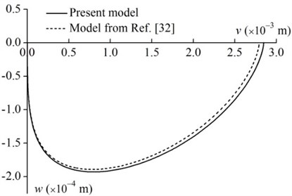
Fig. 3Tip motion trajectories of the rotating rod (m= 0.1 kg, L= 0.8 m and ϖ= 1 rad/s)
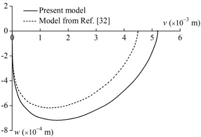
Fig. 3 shows the tip motion trajectories of the rod obtained from the present study and Liu et al. [32] with 1 rad/s. In this calculation, the concentrated mass and the length of the rod are set to 0.1 kg and 0.8 m, respectively, and the other parameters are the same as those in Table 1. It can be seen from Fig. 3 that the results of the present model and Liu’s model [32] have great differences. This reveals that the effect of the mass of the rod on the exact dynamic analysis cannot be neglected.
Table 1The physical parameters of the rotating hub-rod-concentrated mass system for comparative study
Concentrated mass | Rod length | Rod diameter | Young’s modulus | Eccentricity of rod | Mass density of rod |
0.3 kg | 0.3 m | 0.003 m | 100 GPa | 0.1 m | 7.2×10³ kg/m3 |
3.2. Dynamic response analysis for a prescribed rotation
The Eq. (26) is used to determine the elastic deformations of the rod when the rotation of the hub is assumed to be known. A prescribed rotating motion of the hub is defined by:
where denotes the steady-state rotational speed ratio and represents a given dimensionless time parameter. Here 0.2 and 15 are used in this section. According to Eq. (27), the prescribed motion can be divide into four different motion processes. The hub is initially at rest and then a spin-up process is performed from 0 to 15. The steady-state rotational speed ratio is maintained when and the steady-state rotation follows a spin-down process when , finally the rotating motion stops after 45. The variations of the rotational speed ratio and the rotational acceleration ratio of the hub are illustrated in Fig. 4. The rotational acceleration ratio undergoes two up-down changes in the positive and negative directions during and , respectively.
Fig. 4Variations of a) the rotational speed ratio and b) the rotational acceleration ratio of the hub
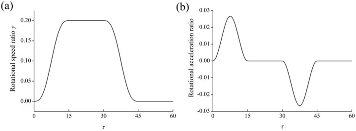
Fig. 5 shows the tip motion trajectory of the rod throughout the whole process of the hub motion prescribed in Eq. (27) with 0.1, 1 and 0.1. During the spin-up process (i.e., ), the tip of the rod moves tangentially backwards ( is negative) and radially outwards, as shown in Fig. 6(a). The radial deformation gradually increases and the tangential deformation increases first and then decreases since the centrifugal force depending on the rotational speed ratio increases and the tangential force depending on the rotational acceleration ratio undergoes an up-down change.
Fig. 5Tip motion trajectory of the rod for the whole process of the hub motion (γ=0.2, T=15, α=0.1, β=1 and δ=0.1)
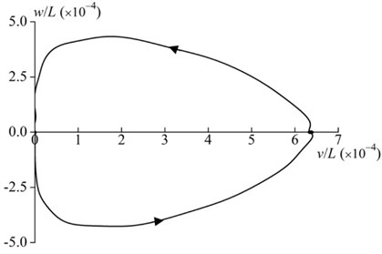
Fig. 6Tip motion trajectory of the rod for the four different motion processes (γ= 0.2, T= 15, α= 0.1, β= 1 and δ= 0.1): a) the spin-up process (0≤τ≤15), b) the steady-state rotation process (15≤τ≤30), c) the spin-down process (30≤τ≤45), d) the static process (τ≥ 45)
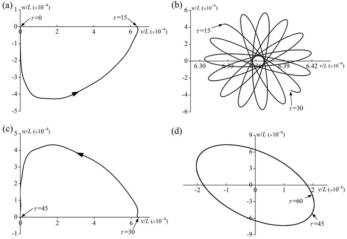
Fig. 6(b) shows the tip motion trajectory of the rod in the steady-state rotation process (i.e., ). An attractive petal pattern is presented since the oval path of the tip trajectory rotates clockwise around a fixed point, which is located in the radial direction. The radial deformation is about two orders of magnitude larger than the tangential deformation. This should be attributed to the fact that the tangential force vanishes due to the steady-state rotation. Therefore, the petal pattern is only affected by Coriolis force.
In the spin-down process (i.e., ), the tip motion trajectory of the rod is displayed in Fig. 6(c). The tip of the rod moves radially inwards and tangentially forwards ( is positive). The radial deformation gradually decreases and the tangential deformation first increases and then decreases.
In the final process (i.e., 45), the hub is at rest so that the motion of the rod is only influenced by its own elastic restoring force. A steady-state tip elliptical motion trajectory of the rod is depicted in Fig. 6(d). This is a typical two-dimensional steady-state oscillation phase diagram.
Fig. 7Effects of parameters on the tip motion trajectory of the rod: a) effect of concentrated mass ratio, b) effect of concentrated mass location ratio, c) effect of initial eccentricity ratio
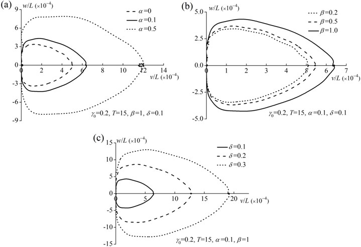
Figs. 7(a), 7(b) and 7(c) show the effects of concentrated mass, concentrated mass location and initial eccentricity ratios on the tip motion trajectories of the rod, respectively. As shown in Fig. 7, both the radial and tangential deformations increase as the concentrated mass, concentrated mass location and initial eccentricity ratios increase due to the increase of the centrifugal force and the tangential force.
3.3. Dynamic response analysis for an arbitrary external torque acting on the hub
For the case of an arbitrary external torque acting on the hub, the rotation of the hub is unknown and should be solved. Evidently, the rigid rotation of the hub can lead to the elastic deformation of the rod, and the elastic deformation of the rod will also affect the rigid rotation of the hub. The Eq. (23) is used to determine the elastic deformations of the rod and the rigid rotation of the hub. The following external torque is assumed to act on the hub:
where is a given external torque ratio. Here, 1 and 40 are fixed to be used. According to Eq. (28), the external torque is acted on the hub following a sinusoidal law during and the external torque is removed when . A numerical example for a rotating hub-flexible circular cross-section rod with a concentrated mass is presented below when 0.5, 1, 0.05, 0.01 and 20.
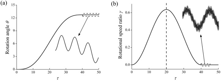
Figs. 8(a) and 8(b) show the responses of the rotation angle and the rotational speed ratio of the hub, respectively. As shown in Fig. 8(a), the rotation angle gradually increases when and then fluctuates within a very small range and decreases slightly when . The rotational speed ratio of the hub increases when , then decreases when and finally oscillates around zero when . As a matter of fact, both the fluctuation of the rotation angle and the oscillation of the rotational speed ratio when that directly reflect the influences of elastic deformations of the rod on the motion of the hub.
Fig. 8Rotation responses of the hub (E-tor0= 1, T= 40, α= 0.5, β= 1, δ= 0.05, d/L=0.01 and ηH= 20): a) the rotation angle, b) the rotational speed ratio
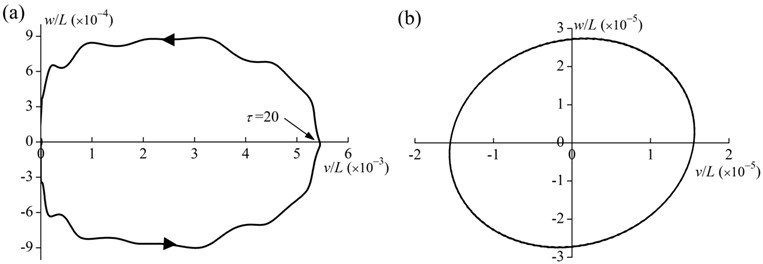
Figs. 9(a) and 9(b) show the tip motion trajectories of the rod for the whole process (i.e., ) and the no external torque process (i.e., ), respectively. As shown in Fig. 9(a), when , the radial deformation gradually increases and the tangential deformation increases first and then decreases to zero. When , the radial deformation gradually decreases and the tangential deformation increases first and then decreases. When , a steady-state tip elliptical motion trajectory is depicted in Fig. 9(b). Obviously, the rotation of the hub causes the corresponding elastic deformations of the rod.
Fig. 9Tip motion trajectory of the rod (E-tor0= 1, T= 40, α= 0.5, β= 1, δ= 0.05, d/L= 0.01 and ηH= 20): a) the whole process (0≤τ≤50), b) the no external torque process (40≤τ≤50)
4. Free vibration analysis for steady-state rotation
In this section, the hub rotates at a constant rotational speed (i.e., ). The free vibration properties of the rotating rod with a concentrated mass could be explored by transforming Eq. (26) into a state space equation, as follows:
where:
in which and are the state space vector and an identity matrix, respectively. Substituting into Eq. (29) yields:
where and are the eigenfrequency and the eigenvector, respectively.
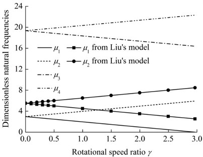
Fig. 10 presents the first four non-dimensional natural frequencies of the rotating rod-concentrated mass system versus rotational speed ratio with 0.1 and 1 alongside the results reported by Liu et al. [32]. As shown in Fig. 10, when 0 (i.e., the hub is at rest), the first and second dimensionless natural frequencies are equal to 2.9678, whereas the results of Liu’s model are 5.4772. Obviously, the consideration of the mass of the rod reduces the natural frequencies of the system. With the increase of the rotational speed ratio, the first and third natural frequencies decrease while the second and fourth natural frequencies increase. The dimensionless fundamental natural frequency vanishes at 2.9678, which is called as the buckling speed ratio. Evidently, the buckling speed ratio of system is equal to the first dimensionless natural frequency of 0. Furthermore, an interesting relationship between the adjacent dimensionless natural frequencies can be obtained as:
where and are the 2th and ()th non-dimensional natural frequencies of the system with the rotational speed ratio , respectively.
Fig. 10The first four dimensionless natural frequencies of the rotating rod-concentrated mass system versus rotational speed ratio (α= 0.1 and β= 1)
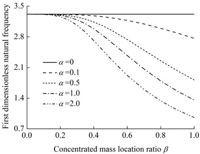
The variation of the dimensionless fundamental natural frequency of the rotating rod-concentrated mass system versus concentrated mass location is depicted in Fig. 11 with 0.2 for five values of 0, 0.1, 0.5, 1.0, 2.0. It is observed from Fig. 11 that the dimensionless fundamental natural frequencies decrease as the concentrated mass location ratio and/or the concentrated mass ratio increase.
Fig. 11The variation of the dimensionless fundamental natural frequency of the rotating rod-concentrated mass system versus concentrated mass location ratio (γ= 0.2)
5. Conclusions
In this study, a comprehensive rigid-flexible coupling dynamic model of a rotating hub-flexible rod with a concentrated mass is established to investigate the dynamic characteristics of the system. On the basis of the classical beam theory and von Kármán geometric nonlinearity, the governing equations of the system are derived by using the Hamilton’s principle. The Galerkin method is employed to solve the derived equations numerically. The rigid-flexible coupling effect between the rigid rotation of the hub and the flexible deformation of the rod leads to the strong nonlinearity of the system. For the case of the prescribed rigid rotation, the dynamic responses of the rod are numerically calculated, and the tip motion trajectories of the rod are graphically presented. The centrifugal, tangential and Coriolis effects on the tip motion trajectories are discussed. The attractive petal pattern for the steady-state rotation and the conventional elliptical pattern for the case without rotation are shown. For the case of the external torque acting on the hub, a numerical example is presented to illustrate the rigid-flexible coupling effect of the system. For the case of steady-state rotation, as the rotational speed ratio increases, the first and third dimensionless natural frequencies decrease and the second and fourth ones increase due to the Coriolis effect. The dimensionless fundamental natural frequency vanishes at the buckling speed ratio. The dimensionless fundamental natural frequency decreases as the concentrated mass location ratio and/or the concentrated mass ratio increase. The modeling method and related conclusions in this paper can provide theoretical basis for the design, optimization and dynamic control of such rotating mechanisms in industrial applications.
References
-
Shabana A. Flexible multibody dynamics: review of past and recent developments. Multibody System Dynamics, Vol. 1, 1997, p. 189-222.
-
Wasfy T., Noor A. Computational strategies for flexible multibody systems. Applied Mechanics Reviews, Vol. 56, Issue 6, 2003, p. 553-613.
-
Schielen W. Computational dynamics: theory and applications of multibody systems. European Journal of Mechanics A-Solids, Vol. 25, Issue 4, 2006, p. 566-594.
-
Singh R., Vandervoort R., Likins P. Dynamics of flexible bodies in tree topology-a computer-oriented approach. Journal of Guidance Control and Dynamics, Vol. 8, Issue 5, 1985, p. 584-590.
-
Kane T. R., Ryan R., Banerjee A. K. Dynamics of a cantilever beam attached to a moving base. Journal of Guidance Control and Dynamics, Vol. 10, Issue 2, 1987, p. 139-151.
-
Krishnaprasad P. S., Marsden J. E. Hamiltonian structures and stability for rigid bodies with flexible attachments. Archive for Rational Mechanics and Analysis, Vol. 98, Issue 1, 1987, p. 71-93.
-
Meirovitch L. Hybrid state equations of motion for flexible bodies in terms of quasi-coordinates. Journal of Guidance Control and Dynamics, Vol. 14, Issue 5, 1991, p. 1008-1013.
-
Choura S., Jayasuriya S., Medick M. A. On the modeling, and open-loop control of a rotating thin flexible beam. Journal of Dynamic Systems, Measurement, and Control, Vol. 113, Issue 1, 1991, p. 26-33.
-
Yokoyama T. Free vibration characteristics of rotating Timoshenko beams. International Journal of Mechanical Sciences, Vol. 30, Issue 10, 1988, p. 743-755.
-
Shahba A., Attarnejad R., Hajilar S. Free vibration and stability of axially functionally graded tapered Euler-Bernoulli beams. Shock and Vibration, Vol. 18, Issue 5, 2011, p. 683-696.
-
Banerjee J. R., Kennedy D. Dynamic stiffness method for inplane free vibration of rotating beams including Coriolis effects. Journal of Sound and Vibration, Vol. 333, Issue 26, 2014, p. 7299-7312.
-
Dehrouyeh-Semnani A.-M. The influence of size effect on flapwise vibration of rotating microbeams. International Journal of Engineering Science, Vol. 94, 2015, p. 150-163.
-
Ghafarian M., Ariaei A. Free vibration analysis of a system of elastically interconnected rotating tapered Timoshenko beams using differential transform method. International Journal of Mechanical Sciences, Vol. 107, 2016, p. 93-109.
-
Azimi M., Mirjavadi S. S., Shafiei N., Hamouda A. M. S., Davari E. Vibration of rotating functionally graded Timoshenko nano-beams with nonlinear thermal distribution. Mechanics of Advanced Materials and Structures, Vol. 25, Issue 6, 2018, p. 467-480.
-
Wright A. D., Smith C. E., Thresher R. W., Wang J. L. C. Vibration modes of centrifugally stiffened beams. Journal of Applied Mechanics, Vol. 49, Issue 1, 1982, p. 197-202.
-
Yoo H. H., Shin S. H. Vibration analysis of rotating cantilever beams. Journal of Sound and Vibration, Vol. 212, Issue 5, 1998, p. 807-828.
-
Li L., Zhang D. G., Zhu W. D. Free vibration analysis of a rotating hub-functionally graded material beam system with the dynamic stiffening effect. Journal of Sound and Vibration, Vol. 333, Issue 5, 2014, p. 1526-1541.
-
Fang J., Zhou D. Free vibration analysis of rotating axially functionally graded tapered Timoshenko beams. International Journal of Structural Stability and Dynamics, Vol. 16, Issue 5, 2016, p. 1550007.
-
Oh Y., Yoo H. H. Vibration analysis of rotating pretwisted tapered blades made of functionally graded materials. International Journal of Mechanical Sciences, Vol. 119, 2016, p. 68-79.
-
Zhao G., Wu Z. Coupling vibration analysis of rotating three-dimensional cantilever beam. Computers and Structures, Vol. 179, 2017, p. 64-74.
-
Fang J., Gu J., Wang H. Size-dependent three-dimensional free vibration of rotating functionally graded microbeams based on a modified couple stress theory. International Journal of Mechanical Sciences, Vol. 136, 2018, p. 188-199.
-
Fang J., Gu J., Wang H., Zhang X. Thermal effect on vibrational behaviors of rotating functionally graded microbeams. European Journal of Mechanics A-Solids, Vol. 75, 2019, p. 497-515.
-
Huang C. L., Lin W. Y., Hsiao K. M. Free vibration analysis of rotating Euler beams at high angular velocity. Computers and Structures, Vol. 88, Issues 17-18, 2010, p. 991-1001.
-
Arvin H., Bakhtiari Nejad F. Non-linear modal analysis of a rotating beam. International Journal of Non-Linear Mechanics, Vol. 46, Issue 6, 2011, p. 877-897.
-
Lacarbonara W., Arvin H., Bakhtiari-Nejad F. A geometrically exact approach to the overall dynamics of elastic rotating blades – part 1: linear modal properties. Nonlinear Dynamics, Vol. 70, Issue 1, 2012, p. 659-675.
-
Kim H., Yoo H. H., Chung J. Dynamic model for free vibration and response analysis of rotating beams. Journal of Sound and Vibration, Vol. 332, Issue 22, 2013, p. 5917-5928.
-
Yang H., Hong J., Yu Z. Dynamics modelling of a flexible hub–beam system with a tip mass. Journal of Sound and Vibration, Vol. 266, Issue 4, 2003, p. 759-774.
-
Liu J. Y., Hong J. Z. Geometric stiffening effect on rigid-flexible coupling dynamics of an elastic beam. Journal of Sound and Vibration, Vol. 278, Issues 4-5, 2004, p. 1147-1162.
-
Cai G. P., Hong J. Z., Yang S. X. Dynamic analysis of a flexible hub-beam system with tip mass. Mechanics Research Communications, Vol. 32, Issue 2, 2005, p. 173-190.
-
You C., Hong J., Cai G. Modeling study of a flexible hub-beam system with large motion and with considering the effect of shear deformation. Journal of Sound and Vibration, Vol. 295, Issues 1-2, 2006, p. 282-293.
-
Li L., Zhang D. Dynamic analysis of rotating axially FG tapered beams based on a new rigid-flexible coupled dynamic model using the B-spline method. Composite Structures, Vol. 124, 2015, p. 357-367.
-
Liu Z., Ye P. X., Guo Y., Guo X. Rigid-flexible coupling dynamic analysis on a mass attached to a rotating flexible rod. Applied Mathematical Modelling, Vol. 38, Issues 21-22, 2014, p. 4985-4994.
-
Zhang D. W., Liu J. K., Huang J. L., Zhu W. D. Periodic responses of a rotating hub-beam system with a tip mass under gravity loads by the incremental harmonic balance method. Shock and Vibration, Vol. 2018, 2018, p. 8178274.
About this article

This research work is supported by the National Natural Science Foundation of China (Grant No. 11872031) and the Natural Science Foundation of Nanjing Institute of Technology (Grant No. ZKJ201701).
